Surviving infant mortality in the hierarchical merging scenario

Abstract

We examine the effects of gas expulsion on initially sub-structured and out-of-equilibrium star clusters. We perform $N$-body simulations of the evolution of star clusters in a static background potential before removing that potential to model gas expulsion. We find that the initial star formation efficiency is not a good measure of the survivability of star clusters. This is because the stellar distribution can change significantly, causing a large change in the relative importance of the stellar and gas potentials. We find that the initial stellar distribution and velocity dispersion are far more important parameters than the initial star formation efficiency, and that clusters with very low star formation efficiencies can survive gas expulsion. We suggest that it is variations in cluster initial conditions rather than in their star formation efficiencies that cause some clusters to be destroyed while a few survive.

1 Introduction

Many, perhaps the vast majority, of stars form in dense, clustered environments (Lada & Lada, 2003; Bressert et al., 2010). However, after only 10 – 20 Myr the vast majority of stars are dispersed into the low density environment of the field (Lada & Lada, 2003). The destruction of most of these early dense clusters has been termed ‘infant mortality’.

Perhaps the best candidate for the mechanism behind infant mortality is primordial gas expulsion. Giant molecular clouds turn only a few per cent to a few tens of per cent of their gas into stars (Lada & Lada, 2003) meaning that the potentials of very young embedded clusters are dominated by gas. Feedback from the most massive stars will remove this gas on a timescale of a few Myr significantly altering the potential of the cluster and potentially leading to its destruction. This process has been studied analytically and with simulations by many authors (e.g. Tutukov, 1978; Hills, 1980; Mathieu, 1983; Elmegreen, 1983; Lada et al., 1984; Elmegreen & Clemens, 1985; Pinto, 1987; Verschueren & David, 1989; Goodwin, 1997a; Goodwin, 1997b; Geyer & Burkert, 2001; Boily & Kroupa, 2003a; Boily & Kroupa, 2003b; Bastian & Goodwin, 2006; Goodwin & Bastian, 2006; Baumgardt & Kroupa, 2007; Parmentier et al., 2008; Goodwin, 2009; Chen & Ko, 2009).

However, previous work has tended to concentrate on clusters that are both in virial equilibrium (notable exceptions are Lada et al., 1984; Elmegreen & Clemens, 1985; Verschueren & David, 1989; Goodwin, 2009) and structurally simple (usually a Plummer sphere or similar). But recent observational and theoretical results strongly suggest that stars do not form in dynamical equilibrium, nor in a smooth distribution (see e.g. Elmegreen & Elmegreen, 2001; Allen et al., 2007; Gutermuth et al., 2009; Bressert et al., 2010 and references in all of these papers). This should not be surprising as in the gravoturbulent model of star formation, stars will form in dense gas in filaments and clumps in a turbulent environment (see e.g. Elmegreen & Scalo, 2004). This has lead to a model of star cluster formation in which a dynamically cool and clumpy initial state collapses and violently relaxes into a dense star cluster (e.g. Allison et al., 2009, Allison et al., 2010).

Strongly non-equilibrium initial conditions may play a crucial role in the effects of gas expulsion on clusters because the key factor in determining the effects of gas expulsion is not only the depth of the gas potential, but also the dynamical state of the stars at the onset of gas expulsion (Verschueren & David, 1989; Goodwin, 2009). As an extreme example, if 99 per cent of the mass of a cluster is expelled, the cluster will still survive if the stars have almost no velocity dispersion.

We might therefore expect the effects of gas expulsion on a cluster to depend on three factors. Firstly, a clumpy and non-symmetrical initial distribution of the stars. Secondly, the star formation efficiency (SFE), and so the relative importance of the stellar and gas potentials. Thridly, the (non-equilibrium) initial conditions of the cluster and the evolution of these initial conditions up until the point of gas expulsion. If clusters are unable to relax fully before gas expulsion then we might expect them to respond very differently to the loss of the residual gas.

In this paper we examine the $N$-body evolution of highly non-equilibrium star cluster in fixed background potentials to model the background gas. The background potential is then removed to simulate the effects of gas expulsion. We describe our initial conditions in Section 2, our results in Section 3, and then discuss the potential consequences in Section 4 before drawing our conclusions in Section 5.

2 Initial conditions

We perform our $N$-body simulations using the Nbody2 code (Aarseth, 2001). Nbody2 is a fast and accurate direct-integration code, optimised for the number of star particles used in this study ($N=1000$). In our simulations there are two separate mass distributions which we wish to model: the stars and the background gas potential.

2.1 Stellar distribution

In all cases we model the stellar distribution as $N=1000$ particles with equal masses of $0.5M_{\odot}$ resulting in a total stellar mass of $500M_{\odot}$. Every particle has a gravitational softening length of 100 AU. We choose softened and equal-mass particles in order to avoid strong two-body interactions and mass segregation. Allison et al. (2009) and Allison et al. (2010) showed that both of these effects can be extremely important in the violent collapse of cool, clumpy regions, however we wish to avoid complicating our simulations with these effects as we are interested in the effects of gas expulsion.

We distribute the stars within a radius of 1.5 pc with two different ‘clumpy’ morphologies: ‘fractal’, and ‘clumpy plummer’. Representative snapshots of the initial conditions of a fractal and clumpy plummer distribution can be seen in the left and right-hand panels, respectively, of Fig. 2.

Fractal clusters are produced using the box fractal technique described by Goodwin & Whitworth (2004); also used by Allison et al. (2009) and Allison et al. (2010). In this paper we use a fractal dimension $D=1.6$ which corresponds to a highly clumpy initial distribution (see Fig. 2).

In clumpy plummers, each sub-clump is modelled as an individual Plummer sphere. The total stellar mass of 500 M_⊙ is distributed into 16 sub-clumps of approximately equal mass. Each sub-clump contains 31.0-31.5 M_⊙ formed from 62-63 particles. The position of individual sub-clumps within the model star forming region follows the gas potential (see below).

2.2 Gas distribution

The gas within the star-forming region is modelled as a static Plummer potential with a mass $M_{\rm{g}}$ and scale-radius $r_{\rm{g}}$.

The scale radius is set to be $r_{\rm{g}}=1$ pc, or $r_{\rm{g}}=1.5$ pc. As the stars have a maximum radius of 1.5 pc this means that for $r_{\rm{g}}=1.5$ pc, the gas distribution seen by the stars is roughly uniform.

The relative masses of the gas potential within 1.5 pc and the stars set the true SFE ($\epsilon$), that is the fraction of the initial cloud mass converted into stars. The mass of the gas potential is varied to obtain true SFEs of 20, 30 and 40 per cent ($M_{\rm{g}}=$2000, 1167, 750 $M_{\odot}$).

Note that a true SFE of 20 or 30 per cent will fail to produce a bound star cluster after instantaneous gas expulsion if the gas and stars are initially virialised (see e.g. Baumgardt & Kroupa, 2007).

We emphasise that the gas potential does not follow the initial stellar distribution, nor does it react to changes in the stellar distribution as it evolves (it is not live). These are obviously extreme simplifications, but as we will discuss later we feel that we capture the essence of the basic physics using such a simple model.

2.3 The dynamical state of the stars

The virial ratio $Q=T/|\Omega|$ is the ratio of the kinetic , $T$, to potential energy, $\Omega$, of the system. We set the initial velocity dispersion of the stars relative to the total potential (gas & stars) to set initial stellar virial ratios between zero (cold), 0.5 (virial equilibrium), and 0.9 (supervirial, but bound).

For initial virial ratios $Q<0.5$, the system will tend to collapse, and for $Q>0.5$ the system will tend to expand. However, even for $Q=0.5$, although the system is in virial equilibrium, the clumpy initial conditions mean that it is not in dynamical equilibrium.

2.4 Gas expulsion

Although young star clusters form embedded within the the molecular gas from which they formed, few star clusters over $\sim 5$ Myr old remain associated with their gas (Proszkow & Adams, 2009). This is likely as a result of a number of mechanisms including radiative feedback from massive stars, stellar winds from young stars, and eventually the onset of the first supernova. The time at which gas removal begins to occur, and the duration of the gas removal process is uncertain, and dependent on the particular gas removal mechanism in operation.

To simulate gas expulsion we instantaneously remove the external gas potential after 3 Myr. This is approximately mid-way between the time at which gas removal from stellar winds and supernova feedback might be expected to occur for star clusters containing $\sim 1000$ stars. Instantaneous gas removal is the most extreme form of gas removal as the stars have no chance to readjust to the change in the potential (e.g. Goodwin, 1997a; Baumgardt & Kroupa, 2007).

2.5 Ensembles

$\begin{array}[]{cc}\includegraphics[height=227.62204pt,width=256.0748pt]{plum1.eps}&\includegraphics[height=227.62204pt,width=256.0748pt]{plum129.eps}\\ \end{array}$

Figure 1: An x-y projection of the initial (left panel) and final (right panel) stellar distribution of an initially clumpy plummer morphology stellar distribution, evolved for 3 Myr in an $r_{\rm{g}}=1$ pc, $M_{\rm{g}}=2000M_{\odot}$ gas potential. The initial virial ratio of the stellar distribution is 0.35. Time of snapshot and LSF at that instant is indicated in top-right hand corner of each panel. The dotted (red) circle marks the stellar half-mass radius, directly used to calculate the $LSF$. In this case, the $LSF$ almost doubles from 0.23 (left panel) to 0.40 (right panel) over the duration of the embedded phase.

It should be noted that both the clumpy plummer and fractal clusters can vary considerably in appearance depending on the random realisation used and the subsequent evolution is highly stochastic (see Allison et al., 2010). We therefore conduct a minimum of 5 random realisations of each parameter set.

2.6 Summary

We set-up clumpy $500M_{\odot}$ star clusters with $N=1000$ equal-mass particles within a static background gas potential. The dynamical state of the stars varies from very cold to almost unbound. The stars dynamically evolve within the gas potential before its instantaneous removal after 3 Myr. We measure the final properties of each star cluster an additional 3 Myr after gas expulsion. A summary of the key parameters is provided in Table 1.

$\begin{array}[]{cc}\includegraphics[width=231.26378pt]{fracrep.eps}&\includegraphics[width=231.26378pt]{plumrep.eps}\\ \end{array}$

Figure 2: Representative examples of an initial distribution of stars with a fractal morphology (left panel), and a clumpy plummer morphology (right panel).

Total mass, $M_{\rm{tot}}$	1250-2500 M⊙*
Outer radius	1.5 pc
Star formation efficiency, $\epsilon$	20-40$\%$*
Total stellar mass, $M_{\rm{star}}$	500 M⊙
Particle number, $N$	1000
Particle mass, $m_{\rm{part}}$	0.5 M⊙
Stellar morphology	fractal or Plummer *
Initial virial ratio, $Q_{\rm{i}}$	0.0-1.0*
Total gas mass, $M_{\rm{g}}$	750-2000 M⊙*
Gas Plummer scale radius, $r_{\rm{g}}$	1.0 pc or 1.5 pc*
crossing-time, $\tau_{\rm{cr}}$	1.4 Myr/2.0 Myr
	($r_{\rm{g}}$=1.0 pc/1.5 pc)

Table 1: The initial conditions parameter sets. Parameters are loosely divided into quantities governing; the total region (upper),the stellar component (middle), the gas component (lower). Parameters that are highlighted with a ‘*’ are parameters we adjust between simulations.

3 Results

We will first discuss the evolution and relaxation of the stellar distribution in the gas potential before addressing the response of the stars to gas expulsion.

3.1 The embedded phase

In all simulations, we evolve our stellar initial conditions for 3 Myr in the gas potential. In Figure 3 we present an example of the evolution of an initially fractal stellar distribution with an initial virial ratio of 0.33 in a gas potential of scale-radius 1 pc. The initial true SFE of this system is $\epsilon=20\%$.

$\begin{array}[]{cc}\includegraphics[height=199.16928pt,width=256.0748pt]{rep1.eps}&\includegraphics[height=199.16928pt,width=256.0748pt]{rep2.eps}\\ \includegraphics[height=199.16928pt,width=256.0748pt]{rep3.eps}&\includegraphics[height=199.16928pt,width=256.0748pt]{rep4.eps}\\ \includegraphics[height=199.16928pt,width=256.0748pt]{rep5.eps}&\includegraphics[height=199.16928pt,width=256.0748pt]{rep6.eps}\\ \end{array}$

Figure 3: The evolution of an initially fractal ($D=1.6$) stellar distribution in an $r_{\rm{g}}=1$ pc, $M_{\rm{g}}=2000M_{\odot}$ gas potential. The initial virial ratio of the stellar distribution is 0.33. The time of each snapshot is indicated in top-right hand corner of each panel.

Clumpy stellar sub-structure interacts resulting in clump merging, and stellar scattering from the clumps (somewhat suppressed in these simulations due to the softening). As a result, substructure is significantly erased on $\sim$1-2 crossing-times of the region. For example, the crossing-time of the region presented in Fig. 3 is 1.4 Myr. By 3 Myr (bottom-right panel) over 2 crossing-times have elapsed, and the remaining stellar distribution has lost most of its sub-structure. Similar behaviour is seen in the simulations of Goodwin & Whitworth (2004), Allison et al. (2009) and Allison et al. (2010). However, they do not include a model for the gas component of the region in their simulations. By including a gas potential in our simulations, the crossing-time of the region is shortened. However the picture of evolution from clumpy substructure to an almost smooth distribution of stars, on timescales of $\sim$1-2 crossing-times of the region, is unsurprisingly unchanged by the presence of the gas.

Importantly, the relaxation and smoothing of the stellar distribution has resulting in it shrinking significantly (see also Allison et al., 2009; Allison et al., 2010). It is clear in Fig.  3 that the central regions of the cluster now contain a greater number of stars than initially. This means that (because the gas potential is static) that the stars are a more significant contributor to the central potential than initially - the effective SFE has increased (Verschueren & David, 1989; Goodwin, 2009) and, in this case, the cluster should be more able to survive gas expulsion.

In order to quantify the effects of collapse (or expansion) and the change of the effective SFE we define the Local Stellar Fraction ($LSF$) of the star forming region:

$$LSF=\frac{M_{\star}(r<r_{\rm{h}})}{M_{\star}(r<r_{\rm{h}})+M_{\rm{gas}}(r<r_{\rm{h}})}.$$ (1)

where $r_{\rm{h}}$ is the radius from the centre of the region containing half the total mass of stars. $M_{\star}$ and $M_{\rm{gas}}$ is the mass of stars and gas, respectively, measured within $r_{\rm{h}}$. Therefore the LSF is a measure of the current effective SFE.

In any non-equilibrium system the half-mass radius of the stars will change with time. Figure 1 shows a projection of the stellar distributions of an initially clumpy plummer model within an $r_{\rm{g}}=1$ pc, $M_{\rm{g}}=2000M_{\odot}$ gas potential. Initially the stars have an initial virial ratio of 0.35, and a half-mass radius $r_{\rm{h}}=0.78$ pc. $LSF=0.23$, close to the initial true SFE of $\epsilon=0.2$ (left panel). However, at 3 Myr the stellar half-mass radius has fallen to $r_{\rm{h}}\sim 0.55$ pc and the $LSF$ is $0.73$ (right panel) - almost double the initial value.

In Figure 4 we plot the $LSF$ measured moments before gas expulsion, versus the initial virial ratio of the stars $Q_{\rm{i}}$. Unsurprisingly, stellar distributions with low initial virial ratio form clusters with high $LSF$s. What is slightly surprising is that high-$Q_{\rm{i}}$ (warm) clusters do not have significantly lower $LSF$s than their initial true SFE. This is because the gas potential dominates and even almost unbound clusters only expand by a factor of less than two in their half-mass radii (some stars are lost, but the half-mass radii do not change by very significant factors). However, there is considerable scatter in the figure. The values with errorbars connected by a solid line in Figure 4 represent the mean values with standard deviation of this scatter in LSF (for $\epsilon=0.2$ simulations) measured in 0.1 wide bins of $Q_{\rm{i}}$. We show a representative histogram for the $Q_{\rm{i}}$=0.3-0.4 bin in Figure 5. On top of our 5 random realisations of each point of our parameter space, we conduct an additional 60 Plummer and 70 fractal morphology simulations so as to ensure a minimum of 20 simulations in each $Q_{\rm{i}}$ bin to avoid low number statistics. The scatter is higher for stellar distributions with low initial virial ratios. This scatter reflects the stochastic nature of cluster evolution from clumpy initial conditions (see Allison et al., 2010).

We find no evidence for any dependency in the position or scatter of the trend on initial stellar morphology (clumpy plummer or fractal) or gas concentration (uniform or concentrated). There is a trend in that clusters with higher true SFEs have higher $LSF$s reflecting their initially higher SFEs (open boxes and triangles in Figure 4).

As well as the $LSF$, the virial ratio of the stars at the onset of gas expulsion is also important. In particular, the velocity dispersion of the stars is crucial, with sub-virial clusters much more able to survive gas expulsion (Goodwin, 2009). Therefore we measure the stellar virial ratio just before gas expulsion $Q_{\rm{pe}}$.

Figure 6 shows the initial and pre-expulsion virial ratios for all our clusters. As would be expected, our clusters have attempted to reach equilibrium (by erasing substructure and collapsing/expanding). In all cases the clusters have reached an approximate virial equilibrium of $Q_{\rm{pe}}\sim 0.5$. However, it is crucial to note that these are approximate equilibriums, and none of these clusters are fully virialised. We shall return to this point later.

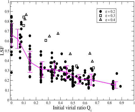
Figure 4: Plot of the initial virial ratio $Q_{\rm{i}}$ against the Local Stellar Fraction ($LSF$) at 3 Myr. Symbols reflect the initial true SFE of the region of 20, 30 or 40 per cent. Initially hot dynamical temperatures result in low $LSF$, and conversely very cold dynamical temperatures result in high $LSF$. At a fixed value of initial virial ratio, there is a slight trend for raised $LSF$ for increasing true SFEs $\epsilon$. Error bars show the mean and standard deviation of the scatter observed in the simulations with an initial true SFE of 20 per cent.

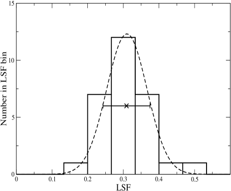
Figure 5: A representative histogram of the scatter in LSF within $Q_{\rm{i}}$ bin 0.1-0.2. Solid bars represent the numbers counted within each LSF bin. The cross point is the average LSF for all clusters within the bin. The error bars of the crossed point are the standard deviation of the LSF scatter. The dashed line shows a gaussian fit with equal standard deviation.

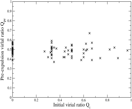
Figure 6: Comparison of the initial virial ratio $Q_{\rm{i}}$, chosen at the beginning of the simulation, versus the pre-gas-expulsion virial ratio $Q_{\rm{pe}}$, measured just prior to gas expulsion. Pre-expulsion virial ratios are all close to virialised ($Q_{\rm{pe}}=0.5$) but scatter around this value with a standard deviation $\sim 0.05$.

3.2 Post-gas-expulsion evolution

After 3 Myr of evolution within the embedded phase (i.e. within the gas background potential), we assume the gas is instantaneously expelled from the star forming region. This is simply modelled by an instantaneous removal of the gas potential. We further evolve the gas-free star cluster an additional 3 Myr after gas expulsion. At this time, we measure the bound mass of the star cluster. Any star whose kinetic energy is less than it’s potential energy is considered bound. We normalise the bound mass by the total stellar mass in the simulation - this quantity is referred to as the bound stellar fraction ($f_{\rm{bound}}$).

In Figure 7 we plot the bound stellar fraction $f_{\rm{bound}}$, as a function of the initial true SFE $\epsilon$. We also plot the results of Baumgardt & Kroupa (2007) (herein BK07) who use initial smooth and virialised equilibrium clusters as their initial conditions.

It is quite clear from this figure that our clusters with an initial true SFE of 20 or 30 per cent can survive gas expulsion with very significant fractions of their initial mass remaining. Also there is a very significant scatter in our results rather than the very tight relationship found by BK07.

We confirm that our choice of 3 Myr of gas free evolution has not significantly influenced our measured bound fraction by evolving a small sub-sample of clusters for 15 Myr after instantaneous gas removal. We continue the gas free evolution phase of three clusters that result in a high ($f_{\rm{bound}}=0.72)$), medium ($f_{\rm{bound}}=0.45)$) and low mass cluster ($f_{\rm{bound}}=0.30)$) when measured after 3 Myr. After 15 Myr, the measured bound fraction differs by $<5\%$ from those measured after 3 Myr.

The differences in our results from those of BK07 are in fact due to the differences in the initial conditions used for the simulations. As we have seen in the previous section, the effective SFE as measured by the $LSF$ can increase significantly before gas expulsion. Rather than expecting a relationship with the initial SFE we should expect a relationship with the $LSF$ which we plot in Fig. 8. Here we find that the final bound fraction of stars does correlate with the $LSF$ in a similar way to the results of BK07. Note that there is no systematic differences between the results of simulations of fractals or clumpy plummers, nor with the concentration of the gas potential.

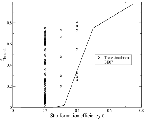
Figure 7: Plot of the region’s SFE $\epsilon$ versus the final cluster’s bound mass fraction $f_{\rm{bound}}$. Crossed symbols are the results of all simulations in this paper, where as the solid line is the results of the BK07 simulations. The points are highly scattered with no clear trend, and do not match the results seen in the BK07 simulations.

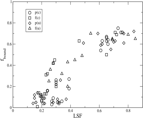
Figure 8: Plot of the influence of $LSF$ (measured at the onset of gas expulsion) on the final bound mass fraction ($f_{\rm{bound}}$) of clusters. All open symbols represent standard model simulations with varying initial stellar morphology or gas potential concentration. Key labels are fractal (f) or clumpy plummer (p) morphology, and uniform (u) or concentrated (c) gas concentration. There is a good trend for increasing bound mass fraction with increasing LSF, although clearly there is scatter in the trend. The trend is independent of initial stellar morphology or gas concentration

However, Figure 8 shows there is still a considerable scatter in the $f_{\rm{bound}}$-$LSF$ trend. Indeed, some clusters with an $LSF$ of $<0.3$ can retain a significant bound fraction of stars after gas expulsion (up to 50 per cent). This is because the $LSF$ is not the only parameter influencing stellar mass loss as a result of gas expulsion. The dynamical state of the cluster, as measured by $Q_{\rm{pe}}$, is also expected to be important (Goodwin, 2009). Recall from Figure 6 - by the onset of gas expulsion all clusters had become approximately virialised. However, even minor deviations from virial equilibrium at the onset of gas expulsion can significantly effect the cluster evolution post-gas-expulsion. In Figure 9, we again plot the $f_{\rm{bound}}$-$LSF$ trend, but this time highlighting simulations whose pre-gas-expulsion virial ratio $Q_{\rm{pe}}$ is greater than 0.55 (super-virial) or less than 0.45 (sub-virial). Clusters that are slightly super-virial at the onset of gas expulsion clearly lie to the lower bounds of $f_{\rm bound}$, whilst those which are sub-virial are at the higher-end.

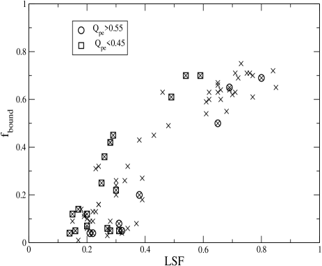
Figure 9: Plot of the influence of the dynamical state of the cluster (as measured by $Q_{\rm{pe}}$) at the time of gas removal. All symbols in Figure 8 (the standard model simulations) are now shown as crosses. Circle and square symbols represent simulations where $Q_{\rm{pe}}>0.55$ or $Q_{\rm{pe}}<0.45$ respectively as indicated in the key.

A gravitational system will reach approximate virial equilibrium in 1 – 2 crossing times, but it will tend to oscillate around exact virial equilibrium for some time (see also Goodwin, 1997a). In Figure 10 we plot the evolution of the virial ratio with time during the embedded phase. We include representative curves for simulations with initial virial ratios of $Q_{\rm{i}}=0.0$, $Q_{\rm{i}}=0.33$, $Q_{\rm{i}}=0.47$ and $Q_{\rm{i}}=0.6$. All curves are results from simulations with a concentrated gas profile with a crossing-time of 1.4 Myr. Whilst all clusters reach approximate virial equilibrium quite quickly they oscillate around $Q=0.5$ for some time. And, as shown in fig. 9, the virial ratio they have at the moment of gas expulsion can make a significant difference to their ability to form a bound cluster afterwards.

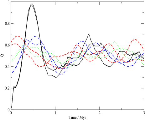
Figure 10: Time evolution of the virial ratio for $Q_{\rm{i}}=0.0$ (solid, black lines), $Q_{\rm{i}}=0.33$ (dot-dash, blue lines), $Q_{\rm{i}}=0.47$ (dotted, green lines), and $Q_{\rm{i}}=0.6$ (dashed, red lines). Colour version available online

4 Discussion

We have shown that initially clumpy and out-of-equilibrium clusters will rapidly relax and erase most of their substructure. Depending on their initial virial ratios and substructure this may mean that they may either collapse or expand. This will alter the importance of the gas potential on the stars meaning that initially cool clusters are more able to survive gas expulsion, whilst initially warm clusters are less likely to. This can remove much of the dependence of survival after gas expulsion from the importance of the initial true SFE and place it instead on the importance of the initial dynamical state of the stars (see also Verschueren & David, 1989; Goodwin, 2009). We have also shown that there is a very significant scatter due to both the intrinsic differences between (statistically the same) clusters (see Allison et al., 2010), and on the exact virial ratio at the onset of gas expulsion.

There is significant observational and theoretical evidence that the initial distributions of stars are not smooth, nor are they virialised (see Elmegreen & Elmegreen, 2001; Bate et al., 2003; Bonnell et al., 2003; Bertout & Genova, 2006; Allen et al., 2007; Kraus & Hillenbrand, 2008; Gutermuth et al., 2009; Clarke, 2010; Bressert et al., 2010 and references in all of these papers) which is a natural consequence of gravoturbulent star formation (see e.g. Elmegreen & Scalo, 2004; McKee & Ostriker, 2007; Bergin & Tafalla, 2007; Clarke, 2010). Indeed, evidence points towards sub-virial initial conditions for stars (see Allison et al. (2010) and references therein). We therefore argue that our initial conditions are far more realistic than those of a smooth, relaxed cluster as generally used before (e.g. Goodwin, 1997a; Goodwin & Bastian, 2006; Baumgardt & Kroupa, 2007).

Proszkow & Adams (2009) conduct a large parameter study investigating the key parameters controlling the final bound fraction of clusters that have undergone gas expulsion using smooth and spherical initial stellar distributions. They find a clear trend with SFE although they, too, use sub-virial initial stellar distributions. We note that we also see a trend for increasing bound fraction with increasing SFE (Figure 7), but that it is highly scattered. The source of this scatter is the use of clumpy initial stellar distribution. Therefore the strength of the star formation efficiency as a predictor for the survival of a cluster to mass loss is severely weakened with the use of far more realistic initially clumpy stellar distributions.

It has often previously been assumed that for a cluster to survive it must have had a high SFE and so the small numbers of clusters we see must be a high-SFE tail to the SFE distribution (see e.g. Parmentier et al., 2008). However, we have shown that some low-SFE clusters can survive if they are ‘lucky’ enough to have the right initial conditions. Indeed, the low survival rates found for young clusters of only $\sim 10$ per cent (Lada & Lada, 2003) may be better explained as these being the few clusters with the ‘right’ initial conditions than being an extremely high-SFE ($>40$ or $50$ per cent) tail of star formation.

We note that our simulations are highly idealised. Stars are equal mass, when Allison et al. (2009) have demonstrated that rapid mass segregation can occur with a more realistic initial mass function.

We do not include any primordial binaries, although their presence can clearly influence the dynamics of a cluster (Goodman & Hut, 1989). The simulations of Kroupa et al. (2001) show that changes in binary fraction, and scattering between stars in the stellar outflow (that can result in binary hardening) can increase the final bound fraction of a cluster. In Moeckel & Bate (2010) the binary fraction does not change significantly during the cluster formation process as a result of formation in an initially high stellar density environment - within sub clumps. However their initial conditions are limited to statistics of one, and we have further demonstrated that clumpy initial conditions can result in highly stochastic behaviour.

Furthermore we assume instantaneous gas removal, although Baumgardt & Kroupa (2007) demonstrate that a slower rate of gas removal can result in a higher cluster survival rate.

The length of the embedded phase is fixed at 3 Myr in our simulations although this could vary depending on the nature of the gas removal mechanism. Despite these simplifications, we argue that the idealised nature of the simulations has enabled us to more clearly test the implications of an initially sub-virial, and clumpy stellar distribution. We defer a less idealised study to a later paper.

Our simulations do have an obvious problem, however, in that we use a smooth, static background potential for the gas. This has two main problems. Firstly, the initial gas and stellar distribution do not match, despite the fact that our stars are assumed to have formed from this background gas. Secondly, the gas is not able to respond to the motion of the stars. (A third, but less important problem, is that we assume that all of the stars form instantaneously.)

The importance of both problems comes down to how well the motions of the gas and the stars are coupled. If conditions are such that both stars and (at least a significant fraction of the) gas move together in the potential then we would expect both to collapse or expand together and the $LSF$ and true star formation efficiency to remain roughly constant. However, if the bulk of the gas does not notice the stars because it is not involved in their formation and the relative gravitational influence of the stars is small, then our approximations should be roughly correct. We would argue that at low true star formation efficiencies that the bulk of the gas would be uncoupled from the stars. We are working on more detailed simulations with a live background potential which we will present in future papers.

5 Summary $\&$ Conclusions

We perform $N$-body simulations of sub-structured, non-equilibrium $500M_{\odot}$ clusters of $N=1000$ equal-mass stars in a static background potential. The mass of gas is varied to simulate star formation efficiencies (SFEs) of 20 to 40 per cent. After 3 Myr of dynamical evolution, the potential is instantaneously removed to model the effect of gas expulsion from the cluster.

Previous work with initially smooth and equilibrium clusters has shown that there is a critical SFE for the survival of (at least part of) the cluster of $\sim 30$ per cent (e.g. Goodwin & Bastian (2006); Baumgardt & Kroupa (2007) and references therein). However, it has also been known that it is the conditions at the onset of gas expulsion that are important in influencing the evolution of the star cluster following gas expulsion (Verschueren & David, 1989, Goodwin, 2009).

Our key results may be summarised as follows.

1. The true SFE is not a good measure of the survival or otherwise of initially out-of-equilibrium clusters. Even though clusters rapidly come into approximate virial equilibrium, their structure can change significantly and, unless the gas follows the motions of the stars, the ratio of gas mass-to-stellar mass quantified by the local stellar fraction ($LSF$) can change hugely.

2. It is the $LSF$, measured at the onset of gas expulsion, that is the key parameter controlling the survival of an embedded cluster to gas expulsion (see Figure 8). A cluster with a high $LSF$ at the onset of gas expulsion – regardless of the initial SFE – is able to produce a cluster with a significant fraction of the initial cluster mass after gas expulsion.

3. The dynamical state of the cluster, as measured by the virial ratio at the onset of gas expulsion, is also important. If gas expulsion occurs when the cluster is mildly sub-virial (i.e. collapsing), the cluster will suffer lower stellar mass loss as a result of gas expulsion. Conversely, a cluster that is mildly super-virial (i.e. expanding) at the onset of gas expulsion suffers greater stellar mass loss during gas expulsion.

The initial SFE of a cluster is almost certainly not a good measure of the ability of a cluster to survive gas expulsion. The initial spacial and kinematic distributions of the stars is crucial, as is how the stars and gas both evolve once the stars have formed. It is quite possible for low-SFE clusters ($<20$ per cent) to produce bound clusters after gas expulsion given the right initial conditions.

References

- Aarseth (2001) Aarseth S. J., 2001, MNRAS, 6, 277
- Allen et al. (2007) Allen L., Megeath S. T., Gutermuth R., Myers P. C., Wolk S., Adams F. C., Muzerolle J., Young E., Pipher J. L., 2007, Protostars and Planets V, pp 361–376
- Allison et al. (2009) Allison R. J., Goodwin S. P., Parker R. J., de Grijs R., Portegies Zwart S. F., Kouwenhoven M. B. N., 2009, ApJL, 700, L99
- Allison et al. (2010) Allison R. J., Goodwin S. P., Parker R. J., Portegies Zwart S. F., de Grijs R., 2010, MNRAS, 407, 1098
- Allison et al. (2009) Allison R. J., Goodwin S. P., Parker R. J., Portegies Zwart S. F., de Grijs R., Kouwenhoven M. B. N., 2009, MNRAS, 395, 1449
- Bastian & Goodwin (2006) Bastian N., Goodwin S. P., 2006, MNRAS, 369, L9
- Bate et al. (2003) Bate M. R., Bonnell I. A., Bromm V., 2003, MNRAS, 339, 577
- Baumgardt & Kroupa (2007) Baumgardt H., Kroupa P., 2007, MNRAS, 380, 1589
- Bergin & Tafalla (2007) Bergin E. A., Tafalla M., 2007, ARA&A, 45, 339
- Bertout & Genova (2006) Bertout C., Genova F., 2006, A&A, 460, 499
- Boily & Kroupa (2003a) Boily C. M., Kroupa P., 2003a, MNRAS, 338, 665
- Boily & Kroupa (2003b) Boily C. M., Kroupa P., 2003b, MNRAS, 338, 673
- Bonnell et al. (2003) Bonnell I. A., Bate M. R., Vine S. G., 2003, MNRAS, 343, 413
- Bressert et al. (2010) Bressert E., Bastian N., Gutermuth R., Megeath S. T., Allen L., Evans II N. J., Rebull L. M., Hatchell J., Johnstone D., Bourke T. L., Cieza L. A., Harvey P. M., Merin B., Ray T. P., Tothill N. F. H., 2010, MNRAS, 409, L54
- Chen & Ko (2009) Chen H., Ko C., 2009, ApJ, 698, 1659
- Clarke (2010) Clarke C., 2010, Royal Society of London Philosophical Transactions Series A, 368, 733
- Elmegreen (1983) Elmegreen B. G., 1983, MNRAS, 203, 1011
- Elmegreen & Clemens (1985) Elmegreen B. G., Clemens C., 1985, ApJ, 294, 523
- Elmegreen & Elmegreen (2001) Elmegreen B. G., Elmegreen D. M., 2001, AJ, 121, 1507
- Elmegreen & Scalo (2004) Elmegreen B. G., Scalo J., 2004, ARA&A, 42, 211
- Geyer & Burkert (2001) Geyer M. P., Burkert A., 2001, MNRAS, 323, 988
- Goodman & Hut (1989) Goodman J., Hut P., 1989, Nature, 339, 40
- Goodwin (1997a) Goodwin S. P., 1997a, MNRAS, 284, 785
- Goodwin (1997b) Goodwin S. P., 1997b, MNRAS, 286, 669
- Goodwin (2009) Goodwin S. P., 2009, Ap&SS, 324, 259
- Goodwin & Bastian (2006) Goodwin S. P., Bastian N., 2006, MNRAS, 373, 752
- Goodwin & Whitworth (2004) Goodwin S. P., Whitworth A. P., 2004, A&A, 413, 929
- Gutermuth et al. (2009) Gutermuth R. A., Megeath S. T., Myers P. C., Allen L. E., Pipher J. L., Fazio G. G., 2009, ApJS, 184, 18
- Hills (1980) Hills J. G., 1980, ApJ, 235, 986
- Kraus & Hillenbrand (2008) Kraus A. L., Hillenbrand L. A., 2008, ApJL, 686, L111
- Kroupa et al. (2001) Kroupa P., Aarseth S., Hurley J., 2001, MNRAS, 321, 699
- Lada & Lada (2003) Lada C. J., Lada E. A., 2003, ARA&A, 41, 57
- Lada et al. (1984) Lada C. J., Margulis M., Dearborn D., 1984, ApJ, 285, 141
- Mathieu (1983) Mathieu R. D., 1983, ApJL, 267, L97
- McKee & Ostriker (2007) McKee C. F., Ostriker E. C., 2007, ARA&A, 45, 565
- Moeckel & Bate (2010) Moeckel N., Bate M. R., 2010, MNRAS, 404, 721
- Parmentier et al. (2008) Parmentier G., Goodwin S. P., Kroupa P., Baumgardt H., 2008, ApJ, 678, 347
- Pinto (1987) Pinto F., 1987, PASP, 99, 1161
- Proszkow & Adams (2009) Proszkow E., Adams F. C., 2009, ApJS, 185, 486
- Tutukov (1978) Tutukov A. V., 1978, A&A, 70, 57
- Verschueren & David (1989) Verschueren W., David M., 1989, A&A, 219, 105