INSTITUT NATIONAL DE RECHERCHE EN INFORMATIQUE ET EN AUTOMATIQUE

A Fully Empirical Autotuned Dense QR Factorization For Multicore Architectures
Emmanuel Agullo — Jack Dongarra — Rajib Nath — Stanimire Tomov N° 7526
 Février 2010 

Abstract: Tuning numerical libraries has become more difficult over time, as systems get more sophisticated. In particular, modern multicore machines make the behaviour of algorithms hard to forecast and model. In this paper, we tackle the issue of tuning a dense QR factorization on multicore architectures. We show that it is hard to rely on a model, which motivates us to design a fully empirical approach. We exhibit few strong empirical properties that enable us to efficiently prune the search space. Our method is automatic, fast and reliable. The tuning process is indeed fully performed at install time in less than one and ten minutes on five out of seven platforms. We achieve an average performance varying from 97% to 100% of the optimum performance depending on the platform. This work is a basis for autotuning the PLASMA library and enabling easy performance portability across hardware systems.

Key-words: Autotuning, empirical tuning, multicore, dense linear algebra, QR factorization

Optimisation automatique entièrement empirique pour la factorisation QR dense sur architectures multi-coeur

Résumé : L’optimisation de librairies numériques est devenue de plus en plus difficile, en même temps que les systèmes se sont complexifiées. En particulier, les machines multi-coeur modernes rendent le comportement des algorithmes difficile à prévoir et modéliser. Dans ce papier, nous étudions le problème de l’optimisation d’une factorisation QR dense sur des architectures multi-coeur. Nous montrons qu’il est difficile d’utiliser un modèle précis, ce qui nous motive pour concevoir une méthode entièrement empirique. Nous mettons en avant quelques propriétés empiriques vérifiées sur un large ensemble de plate-formes. Ces propriétés nous permettent de réduire l’espace de recherche. Notre méthode est automatique, rapide et fiable. Le processus d’optimisation est en effet complètement effectué lors de l’installation de la librairie en moins d’une heure et dix minutes pour cinq des sept plate-formes étudiées. Nous atteigons une performance moyenne variant de 97% à 100% de la performance optimale selon les plate-formes. Ce travail est une base pour l’optimisation automatique de la librairie PLASMA et permettre ainsi la portabilité de sa performance.

Mots-clés : Optimisation automatique, optimisation empirique, multi-coeur, algèbre linéaire dense, factorisation QR

1 Introduction

The hardware trends have dramatically changed in the last few years. The frequency of the processors has been stabilized or even sometimes slightly decreased whereas the degree of parallelism has increased at an exponential scale. This new hardware paradigm implies that applications must be able to exploit parallelism at that same exponential pace [1]. Applications must also be able to exploit a reduced bandwidth (per core) and a smaller amount of memory (available per core). Numerical libraries, which are a critical component in the stack of high-performance applications, must in particular take advantage of the potential of these new architectures. So long as library developers could depend on ever increasing clock speeds and instruction level parallelism, they could also settle for incremental improvements in the scalability of their algorithms. But to deliver on the promise of tomorrow’s petascale systems, library designers must find methods and algorithms that can effectively exploit levels of parallelism that are orders of magnitude greater than most of today’s systems offer. Autotuning is therefore a major concern for the whole HPC community and there exist many successful or on-going efforts. The FFTW library [2] uses autotuning techniques to generate optimized libraries for FFT, one of the most important techniques for digital signal processing. Another successful example is the OSKI library [3] for sparse matrix vector products. The PetaBricks [4] library is a general purpose tuning method providing a language to describe the problem to tune. It has several applications ranging from efficient sorting [4] to multigrid optimization [5]. In the dense linear algebra community, several projects have tackled this challenge on different hardware architectures. The Automatically Tuned Linear Algebra Software (ATLAS) library [6] aims at achieving high performance on a large range of CPU platforms thanks to empirical tuning techniques performed at install time. On graphic processing units (GPUs), among others, [7] and [8] have proposed efficient approaches. FLAME [9] and PLASMA [10] have been designed to achieve high performance on multicore architectures thanks to tile algorithms (see Section 2.1). The common characteristics of all these approaches are that they need intensive tuning to fully benefit from the potential of the hardware. Indeed, the increased degree of parallelism induces a more and more complex memory hierarchy.

Tuning a library consists of finding the parameters that maximize a certain metric (most of the time the performance) on a given environment. In general, the term parameter has to be considered in its broad meaning, possibly including a variant of an algorithm. The search space, corresponding to the possible set of values of the tunable parameters can be very large in practice. Depending on the context, on the purpose and on the complexity of the search space, different approaches may be employed. Vendors can afford dedicated machines for delivering highly tuned libraries [11, 12, 13] and have thus limited constraints in terms of time spent in exploring the search space. On the other side of the spectrum, some libraries such as ATLAS aim at being portable and efficient on a wider range of architectures and cannot afford a virtually unlimited time for tuning. Indeed, empirical tuning is performed at install time and there is thus a trade-off between the time the user accepts to afford to install the library and the quality of the tuning. In that case, the main difficulty consists of efficiently pruning the search space. Of course, once a platform has been tuned, the information can be shared with the community so that it is not necessary to tune again the library, but this is an orthogonal problem which we do not address here. Model-driven tuning may allow one to efficiently prune the search space. Such approaches have been successfully designed on GPU architectures, in the case of matrix vector products [3] or dense linear algebra kernels [7, 8]. However, in practice, the robustness of the assumptions on the model strongly depends both on the algorithm to be tuned and on the target architecture. There is no clearly identified trend yet but model-driven approaches seem to be less robust on CPU architectures. For instance, even in the single-core CPU case, basic linear algebra algorithms tend to need more empirical search [6]. Indeed, on CPU-based architectures, there are many parameters that are not under user control and difficult to model (different levels of cache, different cache policies at each level, possible memory contention, impact of translation lookaside buffers (TLB) misses, …) whereas the current generations of GPU provide more control to the user.

In a previous work, we had tackled the issue of maximizing PLASMA performance in order to compare it against other libraries [14]. We first manually pre-selected a combination of parameters based on the performance of the most compute-intensive kernel. We then tried all these combinations for each considered size of matrix to be factorized. This basic tuning approach achieved high performance but required human intervention to pre-select the parameters and days of run to find optimum performance. In the present paper, not only we now tackle the issue of automatically performing the tuning process but we also present new heuristics that efficiently prune the search space so that the whole tuning process is reduced to one hour or so. We illustrate our discussion with the QR factorization implemented in the PLASMA library, which is representative [14] of all three one-sided factorizations (QR, LU, Cholesky) currently available in PLASMA. Because of the trends expose above and as further motivated in Section 2.3, we do not rely on a model to tune our library. Instead, we employ a fully empirical approach and we exhibit few empirical properties that enable us to efficiently prune the search space.

The rest of the paper is organized as follows. Section 2 presents the problem and motivates the outline of our two-step empirical approach (Section 3). Section 4 presents the wide range of hardware platforms used in the experiments to validate our approach. Section 5 describes the first empirical step, consisting of benchmarking the most compute-intensive serial kernels. We propose three new heuristics that automatically pre-select (PS) candidate values for the tunable parameters. Section 6 presents the second empirical step, consisting of benchmarking effective multicore QR factorizations. We propose a new pruning approach, which we call “prune as you go” (PAYG), that enables to further prune the search space and to drastically reduce the whole tuning process. We conclude and present future work directions in Section 7.

2 Problem Description

2.1 Tile QR factorization

The development of programming models that enforce asynchronous, out of order scheduling of operations is the concept used as the basis for the definition of a scalable yet highly efficient software framework for computational linear algebra applications. In PLASMA, parallelism is no longer hidden inside Basic Linear Algebra Subprograms (BLAS) [15] but is brought to the fore to yield much better performance. We do not present tile algorithms in details (more details can be found [10]) but their principles. The basic idea is to split the initial matrix of order $N$ into $NT\times NT$ smaller square pieces of order $NB$, called tiles. Assuming that $NB$ divides $N$, the equality $N=NT\times NB$ stands. The algorithms are then represented as a Directed Acyclic Graph (DAG) [16] where nodes represent tasks performed on tiles, either panel factorization or update of a block-column, and edges represent data dependencies among them. More details on tile algorithms can be found [10]. PLASMA currently implements three one-sided (QR, LU, Cholesky) tile factorizations. The DAG of the Cholesky factorization is the least difficult to schedule since there is relatively little work required on the critical path. LU and QR factorizations have exactly the same dependency pattern between the nodes of the DAG, exhibiting much more severe scheduling and numerical (only for LU) constraints than the Cholesky factorization. Therefore, tuning the QR factorization is somehow representative of the work to be done for tuning the whole library. In the following, we focus on the QR factorization of square matrices in double precision statically scheduled in PLASMA.

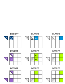
(a) Panel factorization and corresponding updates.

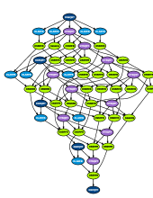
(b) DAG when the matrix is split in $5\times 5$ tiles.

Figure 1: Tile QR Factorization

Similarly to LAPACK which was built using a set of basic subroutines (BLAS), PLASMA QR factorization is built on top of four serial kernels. Each kernel indeed aims at being executed sequentially (by a single core) and corresponds to an operation performed on one or a few tiles. For instance, assuming a $3\times 3$ tile matrix, Figure 1(a) represents the first panel factorization (DGEQRT and DTSQRT serial kernels [10]) and its corresponding updates (DLARFB and DSSRFB serial kernels [10]). The corresponding DAG (assuming this time that the matrix is split in $5\times 5$ tiles) is presented in Figure 1(b).

2.2 Tunable parameters and objective

The shape of the DAG depends on the number of tiles ($NT\times NT$). For a given matrix of order $N$, choosing the tile size NB is equivalent to choosing the number of tiles (since $N=NB\times NT$). Therefore, $NB$ is a first tunable parameter. A small value of $NB$ induces a large number of tasks in the DAG and subsequently enables the parallel processing of many tasks. On the other hand, the serial kernel applied to the tiles needs a large enough granularity in order to achieve a decent performance. The choice of NB thus trades off the degree of parallelism with the efficiency of the serial kernels applied to the tiles. There is a second tunable parameter, called inner block size (IB). It trades off memory load with extra-flops due to redundant calculations. With a value $IB=1$, there are $\frac{4}{3}N^{3}$ operations as in standard LAPACK algorithm. On the other hand, if no inner blocking occurs ($IB=NB$), the resulting extra-flops overhead may represent $25\%$ of the whole QR factorization (see [10] for more details). The general objective of the paper is to address the following problem.

Problem 2.1

Given a matrix size $N$ and a number of cores $ncores$, which tile size and internal blocking size (NB-IB combination) do maximize the performance of the tile QR factorization?

Of course, the performance $P$ we aim at maximizing shall not depend on extra-flops. Therefore, independently of the value of $IB$, we define $P=\frac{4}{3}\times N^{3}/t$, where $t$ is the elapsed time of the QR factorization. Note also that we want the decision to be instantaneous when the user requests to factorize a matrix so that the tuning process is to be performed at install time.

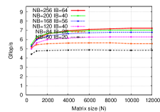
(a) PLASMA QR factorization.

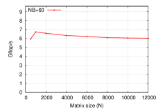
(b) Tile matrix multiplication (GEMM), with tile size $NB=60$.

Figure 2: Performance of the PLASMA QR factorization (left) and tile matrix multiplication (right) on an Intel Core Tigerton machine.

In a sequential execution of PLASMA, parallelism cannot be exploited. In that case, PLASMA’s performance is only related to the performance of the serial kernel which increases with the tile size. Figure 2(a) illustrates this property on an Intel Core Tigerton machine that will be described in details in Section 4.

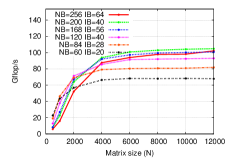
(a) Intel Tigerton machine - 16 cores.

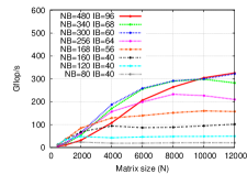
(b) IBM Power6 machine - 32 cores.

Figure 3: Performance of the PLASMA QR factorization

In a parallel execution of PLASMA, the optimum tile size depends on the matrix size as shown on a $16$ cores execution in Figure 3(a). Indeed, if the matrix is small, it needs to be cut in even smaller pieces to provide work to all the $16$ cores even if this induces that the serial kernels individually achieve a lower performance. When the matrix size increases, all the cores may evenly share the work using a larger tile size and thus achieving a higher performance. In a nutshell, the optimum tile size both depends on the number of cores and the matrix size, and its choice is critical for performance. Figure 3(b) shows that the impact is even stronger on a 32 cores IBM Power6 machine, also described in details in Section 4. The 80-40 combination is optimum on a matrix of order $500$ but only achieves $6.3\%$ of the optimum ($20.6$ Gflop/s against $325.9$ Gflop/s) on a matrix of order $12,000$.

2.3 Motivation for an empirical approach

We have just shown the tremendous impact of the tunable parameters on performance. As discussed in Section 1, the two main classes of tuning methods are the model-driven and empirical approaches. We mentioned in the introduction that dense linear algebra algorithms are difficult to model on CPU-based architectures, and in particular on multicore architectures. We now illustrate this claim. Before coming back to the tile QR factorization, we temporarily consider a simpler tile algorithm: the tile matrix multiplication: $C\leftarrow C+A\times B$. Matrices $A$, $B$ and $C$ are split into tiles $a_{ij}$, $b_{ij}$ and $c_{ij}$, respectively. The tile matrix multiplication is then the standard nested loop on sub-arrays $i$, $j$ and $k$ whose single instruction is a DGEMM BLAS call on the corresponding tiles: $c_{ij}\leftarrow c_{ij}+a_{ik}\times b_{kj}$. Given the simplicity of this algorithm (simple DAG, only one kernel, …) one may expect that extrapolating the performance of the whole tile algorithm $C\leftarrow C+A\times B$ from the performance of the BLAS kernel $c_{ij}\leftarrow c_{ij}+a_{ik}\times b_{kj}$ is trivial.

However, the first difficulty is to correctly model how data are accessed during the execution of the tile algorithms. Indeed, before performing the BLAS call, some tiles may be in cache while others are partially or fully out of cache. Figure 4 presents

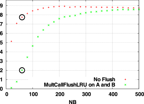
Figure 4: Performance (in Gflop/s) of a sequential matrix multiplication $c\leftarrow c+a\times b$ on the Intel Core Tigerton machine as a standard call to the vendor BLAS library. With the No Flush strategy, data ($a$, $b$ and $c$) is not flushed from the cache. With the MultCallFlushLRU strategy [17], $a$ and $b$ (but not $c$) are flushed from the cache. The values corresponding to a matrix order $NB=60$ are circled.

the impact of the initial state of the tiles on the performance of a sequential matrix multiplication $c\leftarrow c+a\times b$ on the Intel Core Tigerton machine as a DGEMM call to the vendor BLAS library. In the No Flush strategy, all the tiles are initially in cache (if they can fit). On the other hand, in the MultCallFlushLRU [17] strategy, $a$ and $b$ (but not $c$) are flushed from the cache between two successive calls. To achieve accurate timing, we called several times ($50$) the DGEMM kernel for each matrix order ($NB$). The $50$ calls are timed all at once; the average value finally computed is then more accurate than in the case of timing a single call [17]. To simulate the case where data is not flushed, all $50$ executions are performed on the same data [17]. To simulate the case where $a$ and $b$ are flushed, two large arrays $A$ and $B$ are allocated, and the pointers $a$ and $b$ are moved along these arrays between two successive calls. This self-flushing strategy was introduced in [17]. Figure 4 shows that the impact of the initial state is very important. For instance, for a tile of order $NB=60$, the performance is four times higher ($8$ Gflop/s against $2$ Gflop/s) in the No Flush case. In practice, none of these cases is a correct model for the kernel, since the sequential tile multiplication based on a tile size $NB=60$ is neither $8$ nor $2$ Gflop/s but $6$ Gflop/s as shown in Figure 2(b).

This experiment showed that modeling tile algorithms on CPU-based architectures is not trivial, even in the sequential case and even in the case of a simple algorithm such as the matrix multiplication. Parallel execution performance is even more difficult to forecast. For instance, frequent concurrent accesses to the memory bus can slow down the memory controller (as observed for small tile sizes on large matrices in Figure 3(b)). The behavior of shared caches is also difficult to anticipate. On top of that, other algorithmic factors would add up to this complexity in the case of a more complex operation such as a QR factorization. For instance, load balancing issues and scheduling strategies must be taken into account when modeling a tile QR factorization.

As a consequence, we decided to base our approach on an extensive empirical search coupled with only few but strongly reliable properties to prune that search space.

3 Two-step empirical method

Given the considerations discussed in Section 2.3, we do not propose a model-driven tuning approach. Instead we use a fully empirical method that effectively executes the factorizations on the target platform. However, not all NB-IB combinations can be explored. Indeed, an exhaustive search is cumbersome since the search space is huge. For instance, there are more than 1000 possible NB-IB combinations even if we constrain NB to be an even integer lower than 512 (size where the single core compute-intensive kernel reaches its asymptotic performance) and if we impose IB to divide NB. Exploring this search space on a matrix of order $N=10,000$ with 8 cores on the Intel Core Tigerton machine (described in Section 4) would take several days. Therefore, we need to prune the search space. We propose a two-step approach. In Step 1 (Section 5), we benchmark the most compute-intensive serial kernel. This step is fast since the serial kernels operate on tiles, which are of small granularity ($NB<512$) compared to the matrices to be factorized ($500\leq N\leq 10000$ in our study). Thanks to this collected data set and a few well chosen empirical properties, we pre-select (PS) a subset of NB-IB combinations. We propose three heuristics for performing that preliminary pruning automatically. In step 2 (Section 6) we benchmark the effective multicore QR factorizations on the pre-selected set of NB-IB combinations. We furthermore show that further pruning (PAYG) can be performed during this step, drastically reducing the whole tuning process.

4 Experimental environments

To assess the portability and reliability of our method, we consider seven platforms based Intel EM64T processors, IBM Power and AMD x86_64. We recall here that we are interested in shared memory multicore machines. Below is the list of machines used in our experiments.

Intel Core Tigerton. This 16 cores machine is a quad-socket quad-core Xeon E7340 (codename Tigerton) processor, an Intel Core micro-architecture. The processor operates at $2.39$ GHz. The theoretical peak is equal to $9.6$ Gflop/s per core or $153.2$ Gflop/s for the whole node, composed of 16 cores. There are two levels of cache. The level-1 cache, local to the core, is divided into 32 kB of instruction cache and 32 kB of data cache. Each quad-core processor being actually composed of two dual-core Core2 architectures, the level-2 cache has $2\times 4$ MB per socket (each dual-core shares 4 MB). The effective bus speed is 1066 MHz per socket leading to a bandwidth of $8.5$ GB/s (per socket). The machine is running Linux 2.6.30 and provides Intel Compilers 11.0 together with the MKL 10.1 vendor library.

Intel Core Clovertown. This 8 cores server is another machine based on an Intel Core micro-architecture. The machine is composed of two quad-core Xeon X5355 (codename Clovertown) processors, operating at $2.66$ GHz. The theoretical peak is equal to $10.64$ Gflop/s per core and thus $85.12$ Gflop/s for the whole machine. The machine comes with Linux 2.6.28, Intel Compilers 11.0 and MKL 10.1.

Intel Core Yorkfield. This 4 cores desktop is also based on an Intel Core micro-architecture. The machine is composed of one Core 2 Quad Q9300 (codename Yorkfield) processor, operating at $2.5$ GHz. The theoretical peak is equal to $10.0$ Gflop/s per core and thus $40.00$ Gflop/s for the whole machine with a shared 3 MB level-2 cache per core pair. Each core has 64 KB of level-1 cache. The machine comes with Linux 2.6.33, Intel Compilers 11.0 and MKL 10.1.

Intel Core Conroe. This 2 cores desktop is based on an Intel Core micro-architecture too. The machine is composed of one Core 2 Duo E6550 (codename Conroe) processors, operating at $2.33$ GHz. The theoretical peak is equal to $9.32$ Gflop/s per core and thus $18.64$ Gflop/s for the whole machine with a shared 4 MB level-2 cache. Each core has 128 KB of level-1 cache. The machine comes with Linux 2.6.30.3, Intel Compilers 11.1 and MKL 10.2.

Intel Nehalem. This 8 cores machine is based on an Intel Nehalem micro-architecture. Instead of having one bank of memory for all processors as in the case of the Intel Core’s architecture, each Nehalem processor has its own memory. Nehalem is thus a Non Uniform Memory Access (NUMA) architecture. Our machine is a dual-socket quad-core Xeon X5570 (codename Gainestown) running at 2.93GHz and up to 3.33 GHz in certain conditions (Intel Turbo Boost technology). The Turbo Boost was activated during our experiments, allowing for a theoretical peak of $13.32$ Gflop/s per core, i.e., $106.56$ Gflop/s for the machine. Each socket has 8 MB of level-3 cache (that was missing from most Intel Core-based microprocessors such as Tigerton and Clovertown). Each core has 32 KB of level-1 instruction cache and 32 KB of level-1 data cache, as well as 256 KB of level-2 cache. The machine comes with Linux 2.6.28, Intel Compilers 11.1 and MKL 10.2.

AMD Istanbul. This 48 cores machine is composed of eight hexa-core Opteron 8439 SE (codename Istanbul) processors running at 2.8 GHz. Each core has a theoretical peak of $11.2$ Gflop/s and the whole machine $537.6$ Gflop/s. Like the Intel Nehalem, the Istanbul micro-architecture is a ccNUMA architecture. Each socket has 6 MB of level-3 cache. Each processor has a 512 KB level-2 cache and a 128 KB level-1 cache. After having benchmarked the AMD ACML and Intel MKL BLAS libraries, we selected MKL (10.2) which appeared to be slightly faster in our experimental context. Linux 2.6.32 and Intel Compilers 11.1 were also used.

IBM Power6. This 32 cores machine is composed of sixteen dual-core IBM Power6 processors running at $4.7$ GHz. The theoretical peak is equal to $18.8$ Gflop/s per core and $601.6$ Gflop/s for the whole node. There are three levels of cache. The level-1 cache, local to the core, can contain 64 kB of data and 64 kB of instructions; the level-2 cache is composed of 4 MB per core, accessible by the other core; and the level-3 cache is composed of 32 MB common to both cores of a processor with one controller per core (80 GB/s). The memory bus (75 GB/s) is shared by the 32 cores of the node. The machine runs AIX 5.3 and provides the xlf 12.1 and xlc 10.1 compilers together with the Engineering Scientific Subroutine Library (ESSL) [12] 4.3 vendor library.

5 Step 1: Benchmarking the most compute-intensive serial kernel

Table 1: Elapsed time (hh:mm:ss) for Step 1 and Step 2

Machine		Step 1	Step 2
Architecture	# cores		Heuristic	PS	PSPAYG
			0	14:46:37	03:05:41
Conroe	2	00:24:33	1	09:01:08	00:01:58
			2	07:30:53	00:34:47
			0	17:40:00	04:48:13
Yorkfield	4	00:20:57	1	09:30:30	00:05:10
			2	08:01:05	02:58:37
			0	20:08:43	02:56:25
Clovertown	8	00:21:44	1	11:06:18	00:13:09
			2	08:52:24	01:10:53
			0	06:20:16	01:51:30
Nehalem	8	00:16:29	1	06:20:16	01:51:30
			2	06:20:16	01:51:30
			0	23:29:35	03:15:41
Tigerton	16	00:34:18	1	12:22:06	00:08:57
			2	09:54:59	01:01:06
			0	21:09:27	02:53:38
Istanbul	48	00:24:23	1	12:25:30	00:11:01
			2	10:04:46	00:54:51
			0	03:06:05	00:25:07
Power6	32	00:15:23	1	03:06:05	00:25:07
			2	03:06:05	00:25:07

We explained in Section 2.1 that the tile QR factorization consists of four serial kernels. However, the number of calls to DSSRFB is proportional to $NT^{3}$ while the number of calls to the other kernels is only proportional to $NT$ (DGEQRT) or to $NT^{2}$ (DTSQRT and DLARFB). Even on small DAGS (see Figure 1(b)), calls to DSSRFB are predominant. Therefore, the performance of this compute-intensive kernel is crucial. DSSRFB’s performance also depends on NB-IB. It is thus natural to pre-select NB-IB pairs that allow a good performance of DSSRFB before benchmarking the QR factorization itself. The practical advantage is that a kernel is applied at the granularity of a tile, which we assume to be bounded by $512$ ($NB\leq 512$). Consequently, preliminary benchmarking this serial kernel can be done exhaustively in a reasonable time. Step 1 thus consists of performing an exhaustive benchmarking of the DSSRFB kernel on all possible NB-IB combinations and then to decide which of these will be kept for further testing in Step 2. To achieve accurate timing, we followed the guidelines of [17] as presented in Section 2.3. In particular, DSSRFB is called $50$ times for each $(NB,IB)$ pair. We implemented both No Flush and MultCallFlushLRU strategies. In this paper, we present results related to the No Flush approach. The reason is that it runs faster and provides satisfactory results as we will show. A comparison of both approaches is out of the scope of this manuscript. Column “Step 1” of Table 1 shows that the total elapsed time for step 1 is acceptable on all the considered architectures (between $16$ and $35$ minutes). Figure 5(a) shows the resulting set of empirical data collected during step 1 on the Intel Core Tigerton machine.

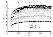
(a) Different NB-IB combinations with a common NB value have the same abscisse; “Max IB” represents the one that achieves the maximum performance among them.

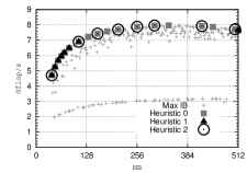
(b) Combinations pre-selected (PS) for each heuristic.

Figure 5: Performance of the DSSRFB serial kernel depending on the NB-IB combination.

This data set can be pruned a first time. Indeed, contrary to NB, which trades off parallelism for kernel performance, IB only affects kernel performance but not parallelism. We can thus perform the following orthogonal optimization:

Property 5.1 (Orthogonal pruning)

For a given NB value, we can safely pre-select the value of IB that maximizes the kernel performance.

Applying Property 5.1 to the data set of Figure 5(a) results in discarding all NB-IB pairs except the ones matching “Max IB”, which still represents a large number of combinations. We thus propose and assess three heuristics to further prune the search space. The first considered heuristic is based on the fact that a search performed with a well chosen subset of a limited number - say 8 - of NB-IB combinations is enough to consistently achieve a maximum performance for any matrix size $N$ or number of cores $ncores$ [14]. Further intensive experiments led to the following property.

Property 5.2 (Convex Hull)

There is consistently an optimum combination on the convex hull of the data set.

Therefore, Heuristic 0 consists of pre-selecting the points from the convex hull of the data set (see Figure 5(b)). In general, this approach may still provide too many combinations. Because NB trades off kernel efficiency with parallelism, the gains observed on kernel efficiency shall be considered relatively to the increase of NB itself. Therefore, we implemented Heuristic 1 that pre-selects the points of the convex hull with a high steepness (or more accurately a point after a segment with a high steepness). The drawback is that all these points tend to be located in the same area as shown in Figure 5(b) corresponding to small values of NB. To correct this deficiency, we consider Heuristic 2 which first divides the x-axis into iso-segments and pick up the point of maximum steepness on each of these segments (see Figure 5(b) again). Heuristics 1 and 2 are paremetrized to select a maximum of 8 combinations. All three heuristics perform a pre-selection (PS) that will be used as test cases for the second step.

6 Step 2: Benchmarking the whole QR factorization

6.1 Discretization and interpolation

We recall that our objective is to immediately retrieve at execution time the optimum NB-IB combination for the matrix size $N$ and number of cores $ncores$ that the user requests. Of course, $N$ and $ncores$ are not known yet at install time. Therefore, the ($N$,$ncores$) space to be benchmarked has to be discretized. We decided to benchmark all the powers of two cores ($1$, $2$, $4$, $8$, …) plus the maximum number of cores in case it is not a power of two such as on the AMD Istanbul machine. The motivation comes from empirical observation. Indeed, Figures 6 and 7 show that the optimum NB-IB combination can be finely interpolated with such a distribution. We discretized more regularly the space on $N$ because the choice of the optimum pair is much more sensible to that dimension (see figures 3(a) and 3(b)). We benchmarked N=500, 1000, 2000, 4000, 6000, 8000, 10000. Each run is performed $6$ times to attenuate potential perturbations. When the user requests the factorization of parameters that have not been tuned (for instance N=1800 and ncores=5) we simply interpolate by selecting the parameters of the closest configuration benchmarked at install time (N=2000 and ncores=4 in that case).

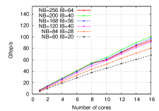
(a) Intel Tigerton machine

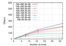
(b) IBM Power6 machine.

Figure 6: Strong scalability - $N=6000$.

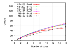
(a) Intel Tigerton machine

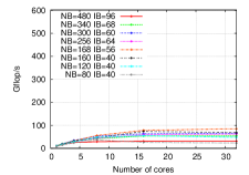
(b) IBM Power6 machine.

Figure 7: Strong scalability - $N=2000$.

6.2 Impact of the pre-selection on the elapsed time of step 2

Column PS (pre-selection) in Table 1 shows the impact of the heuristics (applied at step 1) on the time required for benchmarking step 2. Clearly Heuristic 0 induces a very long step 2 (up to 1 day). Heuristic 1 and 2 induce a lower time for step 2 (about $10$ hours) but that may be still not acceptable for many users.

6.3 Prune As You Go (PSPAYG)

To further shorten step 2, we can perform complementary pruning on the fly. Indeed, figures 3(a) and 3(b) show the following property.

Property 6.1 (Monotony)

Let us denote by $P(NB_{1},N)$ and $P(NB_{2},N)$ the performances obtained on a matrix of order $N$ with tile sizes $NB_{1}$ and $NB_{2}$, respectively. If $P(NB_{1},N)>P(NB_{2},N)$ and $NB_{1}>NB_{2}$, then $P(NB_{1},N^{\prime})>P(NB_{2},N^{\prime})$ for any $N^{\prime}>N$.

We perform step 2 in increasing order of $N$. After having benchmarked the current set of NB-IB combinations on a matrix of order $N$, we identify all the couples $(NB_{1},NB_{2})$ that satisfy Property 6.1 and we remove from the current subset the NB-IB pair in which $NB_{2}$ is involved. Indeed, according to Property 6.1, it would lead to a lower performance than $NB_{1}$ on larger values of $N$ which are going to be explored next. We denote this strategy by “PSPAYG” (pre-selection and prune as you go). Column PSPAYG in Table 1 shows that the time for step 2 is dramatically improved with this technique. Indeed, the number of pairs to explore decreases when $N$ increases, that is, when benchmark is costly. For heuristic 2 (values in bold in Table 1), the time required for step 2 is reduced by a factor greater than $10$ in two cases (Intel Core Conroe and AMD Istanbul machines).

6.4 Reliability

We employed the following methodology to assess the reliability of the different tuning approaches. We first executed all the discussed approaches on all the platforms with the discretization of the ($N$,$ncores$) space proposed in Section 6.1. We then picked up between 8 and 16 ($N$,$ncores$) combinations such that half of them were part of the discretized space (for instance $N=6000$ and $ncores=32$) and the other half were not part of it (for instance $N=4200$ and $ncores=30$) so that the reliability of the interpolation is also taken into account. For each combination we performed an (almost) exhaustive search for reference. Detailed results are provided in Appendix A and we now discuss the synthesis of the results gathered in Table 2. Heuristic 2 coupled with the PSPAYG approach is very efficient since it achieves a high proportion of the performance that would be obtained with an exhaustive search (values in bold). The worst case occurs on the Istanbul machine, with an average relative performance of $97.1\%$ (Column “avg”). However, even on that platform, the optimum NB-IB combination was found in seven cases out of sixteen tests (Column “optimum”).

Column $\frac{PSAYG}{PS}$ allows to specifically assess the impact of the “prune as you go” method since they compare the average performance obtained with PSPAYG (where pairs can be discarded during step 2 according to Property 6.1) compared to PS (where no pair is discarded during step 2). The result is clear: pruning during step 2 according to Property 6.1 does not hurt performance ($\frac{|PS-PSPAYG|}{PS}<0.3\%$), showing that Property 6.1 is strongly reliable. Finally, note that on ($N$,$ncores$) combinations part of the discretized space, PSPAYG cannot achieve a higher performance than PS since all NB-IB combinations tested with PSPAYG are also tested with PS. However, PSPAYG can achieve a higher performance if ($N$,$ncores$) was not part of the discretized space because of the interpolation. This is why cases where $\frac{PSPAYG}{PS}>100\%$ may be observed.

Table 2: Average performance achieved with a “pre-selection” (PS) method or a “pre-selection and prune as you go” (PSPAYG) method, based on different heuristics (H) applied at step 1. The performance is presented as a proportion of the exhaustive search (ES) or of the prunes search (PS). The column “optimum” indicates the number of times the optimum combination (with respect to the reference method) was found among the number of tests performed.

		$\frac{PS}{ES}$(%)		$\frac{PSPAYG}{ES}$(%)		$\frac{PSPAYG}{PS}(\%)$
Machine	H	avg	optimum	avg	optimum	avg	optimum
	0	99.67	6/8	99.67	6/8	100	8/8
Conroe	1	95.28	0/8	95.28	0/8	100	8/8
	2	99.54	5/8	99.54	5/8	100	8/8
	0	98.63	6/12	98.63	6/12	100	12/12
Yorkfield	1	91.53	0/12	91.59	0/12	100.07	10/12
	2	98.63	6/12	98.63	6/12	100	12/12
	0	98.59	8/16	98.35	7/16	99.76	15/16
Clovertown	1	91.83	0/16	91.83	0/16	100	16/16
	2	98.49	9/16	98.25	8/16	99.76	15/16
	0	98.6	8/16	98.9	8/16	100.33	16/16
Nehalem	1	98.6	8/16	98.9	8/16	100.33	16/16
	2	98.6	8/16	98.9	8/16	100.33	16/16
	0	97.36	8/16	97.54	5/16	100.21	12/16
Tigerton	1	91.61	0/16	91.61	0/16	100	16/16
	2	97.51	8/16	97.79	7/16	100.31	15/16
	0	97.17	7/16	97.17	7/16	100	16/16
Istanbul	1	94.12	2/16	94.12	2/16	100	16/16
	2	97.23	7/16	97.1	7/16	99.87	15/16
	0	100	16/16	100	16/16	100	16/16
Power 6	1	100	16/16	100	16/16	100	16/16
	2	100	16/16	100	16/16	100	16/16

7 Conclusion

We have presented a new fully autotuned method for dense linear algebra libraries on multicore architectures. We have validated our approach thanks to the PLASMA library on a wide range of architectures representative of today’s HPC CPU trends. We have illustrated our discussion with the QR factorization, which is representative of the difficulty of tuning any of the three one-sided factorizations (QR, LU, Cholesky) present in PLASMA.

We have recalled that tuning consists in exploring a search space of tunable parameters. In general, the exploration can be pruned thanks to model-driven considerations. For our particular problem, we have experimentally exhibited the weak reliability of the behavior of dense linear algebra operations on modern multicore architectures. It motivated us to use extensive empirical search coupled with only few but strongly reliable properties to prune that search space. The experimental validation has shown that the whole autotuning process can in general be brought to completion in a decent time (less than one hour and ten minutes on five out of seven platforms) though allowing to achieve a very high performance (often finding the optimum tunable parameters and achieving at least $97\%$ of the optimum performance in average on each machine) on a wide range of architectures.

Our approach is user-friendly. At install time, the PLASMA library is installed with default tunable parameters. A simple make autotune launches the empirical benchmarking steps and builds the decision tree based on simple interpolation properties. When the end-user calls the library, the pre-built decision tree is used to choose the optimized tunable parameters found at install time. The process did not require any human intervention except on the IBM platform. Indeed, we have had to manually arrange the tuning process in order to cope with the batch scheduler (LoadLeveler [18]) used to submit the jobs on that IBM machine. We are currently working on a better integration of the autotuning process with machines ruled by batch schedulers.

We have considered the factorization of square matrices. The factorization of non square matrices has to be studied too. In particular, the case of tall and skinny matrices (which have a larger number of rows than columns) often arises in several important applications [19]. In [20], the authors have shown that communication-avoiding algorithms [19] are well adapted for processing such matrices in a multicore context. They consist of splitting further the matrix in multiple block rows (called domains) to enhance parallelism. The number $p$ of domains is another tunable parameter that combines with NB and IB and should thus be integrated in the empirical search method.

Hybrid multicore platforms with GPU accelerators tend to be more and more frequent [21]. The ultimate goal being to develop a library that furthermore goes at scale when increasing the number of nodes [22], the natural suite of the work presented in that paper is to propose a unified framework for tuning dense linear algebra libraries on modern hardware (distributed memory, multicore micro-architectures and GPU accelerators). However, the issues to be addressed, being very different from one type of hardware to another, must take into account the particularities of each type of hardware. In that respect, the method presented in this document can be used as a building block for such a unified framework.

Appendix A Detailed results for Step 2

We now present more detailed performance results to explain more accurately how the synthetic results of Table 2 were obtained. We illustrate our discussion with performance results of the AMD Istanbul machine (tables 3, 4, 5 and 6). To assess the efficiency of the different methods presented in the paper, we have performed between $8$ and $16$ tests on each machine. Each test is an evaluation of the method for a given number of cores $ncores$ and a matrix size $N$. On the AMD Istanbul machine, the $16$ possible combinations of N = 2000, 2700, 4200 or 6000 and $ncores$ = 4, 7, 40 or 48 have been tested. An exhaustive search (ES) is first performed for all these $16$ combinations to be used as a reference (Table 3). Then we test which NB-IB combination would have been chosen by the autotuner depending on the method it is built on (tables 4, 5 and 6).

We comment more specifically the results obtained for Heuristic 2 (Table 6) since it is the heuristic that we plan to set as a default in PLASMA. The first four rows show results related to experimental conditions in which both the matrix order and the number of cores are part of the values that were explicitly benchmarked during the tuning process (N=2000 or 6000 and $ncores$=4 or 48). No interpolation is needed. In three cases, the optimum configuration is found both by PS and PSPAYG. In the case were it was not found (N=6000 and ncores=4) the optimum configuration was actually not part of the initial pre-selected points by Heuristic 2 (Y=0). The four next rows (N=2700 or 4200 and $ncores$=4 or 48) require to interpolate the matrix order (but not the number of cores). For N=2700, the selection is based on the benchmarking realized on $N_{0}$=2000 while $N_{0}$=4000 is chosen when $N=4200$. The achieved performance is not ideal since it is $8\%$ lower than the exhaustive search. As expected, the interpolation on $ncores$ is much less critical (four next rows). This observation confirms the validity of a discretization coarser on the $ncores$ dimension. Finally (last four rows), the quality of the tuning for the interpolation in both dimensions is comparable to the one related to the interpolation on $N$.

Table 3: Performance of ES on the AMD Istanbul Machine

N	ncore	Perf (Gflop/s)	NB	IB
2000	4	24.81	168	28
2000	48	140.1	96	32
6000	4	30.36	504	56
6000	48	272.55	168	28
2700	4	26.35	300	60
2700	48	176.7	108	36
4200	4	28.65	480	60
4200	48	239.93	128	32
2000	7	40.31	168	28
2000	40	135.72	96	32
6000	7	50.41	300	60
6000	40	236.8	168	28
2700	7	44.13	180	36
2700	40	168.79	108	36
4200	7	48.44	300	60
4200	40	213.27	168	28

Table 4: Performance of Heuristic 0 on the AMD Istanbul machine.

N	ncore	Y	PS	$\frac{PS}{ES}\%$	PSPAYG	$\frac{PSPAYG}{ES}\%$	$\frac{PSPAYG}{PS}\%$
2000	4	1	24.81	100	24.81	100	100
2000	48	1	140.1	100	140.1	100	100
6000	4	1	30.36	100	30.36	100	100
6000	48	1	272.55	100	272.55	100	100
2700	4	1	24.24	92	24.24	92	100
2700	48	1	169.32	95.83	169.32	95.83	100
4200	4	1	26.8	93.52	26.8	93.52	100
4200	48	1	237.19	98.86	237.19	98.86	100
2000	7	1	40.31	100	40.31	100	100
2000	40	1	126.66	93.32	126.66	93.32	100
6000	7	1	50.36	99.9	50.36	99.9	100
6000	40	1	236.8	100	236.8	100	100
2700	7	1	40.4	91.56	40.4	91.56	100
2700	40	1	164.76	97.61	164.76	97.61	100
4200	7	1	44.64	92.16	44.64	92.16	100
4200	40	1	213.27	100	213.27	100	100

Table 5: Performance of Heuristic 1 on the AMD Istanbul machine

N	ncore	Y	PS	$\frac{PS}{ES}\%$	PSPAYG	$\frac{PSPAYG}{ES}\%$	$\frac{PSPAYG}{PS}\%$
2000	4	0	22.84	92.06	22.84	92.06	100
2000	48	1	140.1	100	140.1	100	100
6000	4	0	29.47	97.07	29.47	97.07	100
6000	48	0	256.42	94.08	256.42	94.08	100
2700	4	0	22.9	86.92	22.9	86.92	100
2700	48	1	169.32	95.83	169.32	95.83	100
4200	4	0	25.87	90.28	25.87	90.28	100
4200	48	1	239.93	100	239.93	100	100
2000	7	0	36.92	91.57	36.92	91.57	100
2000	40	1	126.66	93.32	126.66	93.32	100
6000	7	0	49.07	97.35	49.07	97.35	100
6000	40	0	224.13	94.65	224.13	94.65	100
2700	7	0	38.83	88	38.83	88	100
2700	40	1	164.76	97.61	164.76	97.61	100
4200	7	0	43.04	88.85	43.04	88.85	100
4200	40	0	209.74	98.34	209.74	98.34	100

Table 6: Performance of Heuristic 2 on the AMD Istanbul machine

N	ncore	Y	PS	$\frac{PS}{ES}\%$	PSPAYG	$\frac{PSPAYG}{ES}\%$	$\frac{PSPAYG}{PS}\%$
2000	4	1	24.81	100	24.81	100	100
2000	48	1	140.1	100	140.1	100	100
6000	4	0	29.98	98.75	29.35	96.66	97.89
6000	48	1	272.55	100	272.55	100	100
2700	4	1	24.24	92	24.24	92	100
2700	48	0	169.32	95.83	169.32	95.83	100
4200	4	1	26.8	93.52	26.8	93.52	100
4200	48	0	237.19	98.86	237.19	98.86	100
2000	7	1	40.31	100	40.31	100	100
2000	40	1	135.72	100	135.72	100	100
6000	7	1	50.36	99.9	50.36	99.9	100
6000	40	1	236.8	100	236.8	100	100
2700	7	0	40.4	91.56	40.4	91.56	100
2700	40	0	157.06	93.05	157.06	93.05	100
4200	7	1	44.64	92.16	44.64	92.16	100
4200	40	1	213.27	100	213.27	100	100

Contents

1. 1 Introduction
2. 2 Problem Description
   1. 2.1 Tile QR factorization
   2. 2.2 Tunable parameters and objective
   3. 2.3 Motivation for an empirical approach
3. 3 Two-step empirical method
4. 4 Experimental environments
5. 5 Step 1: Benchmarking the most compute-intensive serial kernel
6. 6 Step 2: Benchmarking the whole QR factorization
   1. 6.1 Discretization and interpolation
   2. 6.2 Impact of the pre-selection on the elapsed time of step 2
   3. 6.3 Prune As You Go (PSPAYG)
   4. 6.4 Reliability
7. 7 Conclusion
8. A Detailed results for Step 2

References

- [1] H. Sutter. A fundamental turn toward concurrency in software. Dr. Dobb’s Journal, 30(3), 2005.
- [2] M. Frigo and S. Johnson. FFTW: An adaptive software architecture for the FFT. In Proc. 1998 IEEE Intl. Conf. Acoustics Speech and Signal Processing, volume 3, pages 1381–1384. IEEE, 1998.
- [3] Jee Whan Choi, Amik Singh, and Richard W. Vuduc. Model-driven autotuning of sparse matrix-vector multiply on GPUs. In Proc. ACM SIGPLAN Symp. Principles and Practice of Parallel Programming (PPoPP), Bangalore, India, January 2010.
- [4] Jason Ansel, Cy Chan, Yee Lok Wong, Marek Olszewski, Qin Zhao, Alan Edelman, and Saman Amarasinghe. Petabricks: A language and compiler for algorithmic choice. In ACM SIGPLAN Conference on Programming Language Design and Implementation, Dublin, Ireland, Jun 2009.
- [5] Cy Chan, Jason Ansel, Yee Lok Wong, Saman Amarasinghe, and Alan Edelman. Autotuning multigrid with petabricks. In ACM/IEEE Conference on Supercomputing, Portland, OR, Nov 2009.
- [6] R. Clint Whaley, Antoine Petitet, and Jack J. Dongarra. Automated empirical optimizations of software and the atlas project. Parallel Computing, 27(1-2):3 – 35, 2001.
- [7] Vasily Volkov and James W. Demmel. Benchmarking gpus to tune dense linear algebra. In SC ’08: Proceedings of the 2008 ACM/IEEE conference on Supercomputing, pages 1–11, Piscataway, NJ, USA, 2008. IEEE Press.
- [8] S. Tomov, R. Nath, H. Ltaief, and J. Dongarra. Dense linear algebra solvers for multicore with gpu accelerators. Accepted for publication at HIPS 2010, 2010.
- [9] G. Quintana-Ortí, E. Quintana-Ortí, R. van de Geijn, F. Van Zee, and E. Chan. Programming matrix algorithms-by-blocks for thread-level parallelism. ACM Trans. Math. Softw., 36(3), 2009.
- [10] A. Buttari, J. Langou, J.Kurzak, and J.Dongarra. A class of parallel tiled linear algebra algorithms for multicore architectures. Parallel Computing, 35(1):38–53, 2009.
- [11] Intel, Math Kernel Library (MKL). http://www.intel.com/software/products/mkl/.
- [12] IBM, Engineering and Scientific Subroutine Library (ESSL) and Parallel ESSL. http://www-03.ibm.com/systems/p/software/essl/.
- [13] Short Contents. Amd core math library (acml).
- [14] Emmanuel Agullo, Bilel Hadri, Hatem Ltaief, and Jack Dongarra. Comparative study of one-sided factorizations with multiple software packages on multi-core hardware. 2009 International Conference for High Performance Computing, Networking, Storage, and Analysis (SC ’09), 2009.
- [15] BLAS: Basic Linear Algebra Subprograms. http://www.netlib.org/blas/.
- [16] N. Christofides. Graph Theory: An algorithmic Approach. New York: Academic Press, 1975.
- [17] C. Whaley and M. Castaldo. Achieving accurate and context-sensitive timing for code optimization. Software: Practice and Experience, 38(15):1621–1642, 2008.
- [18] IBM LoadLeveler for AIX 5L. First Edition, December 2001.
- [19] James W. Demmel, Laura Grigori, Mark Frederick Hoemmen, and Julien Langou. Communication-optimal parallel and sequential QR and LU factorizations. LAPACK Working Note 204, UTK, August 2008.
- [20] B. Hadri, H. Ltaief, E. Agullo, and J. Dongarra. Tile QR Factorization with Parallel Panel Processing for Multicore Architectures. In Proceedings of the 24th IEEE International Parallel and Distributed Processing Symposium, Atlanta, GA, April 19-23, 2010.
- [21] Emmanuel Agullo, Cédric Augonnet, Jack Dongarra, Mathieu Faverge, Hatem Ltaief, Samuel Thibault, and Stanimire Tomov. QR Factorization on a Multicore Node Enhanced with Multiple GPU Accelerators. In 25th IEEE International Parallel & Distributed Processing Symposium, Anchorage États-Unis, 05 2011.
- [22] George Bosilca, Aurelien Bouteiller, Anthony Danalis, Thomas Herault, Pierre Lemarinier, and Jack Dongarra. "DAGuE: A generic distributed dag engine for high performance computing,". Technical Report ICL-UT-10-01, UTK, April 2010.