Formation of defects in multirow Wigner crystals

Abstract

We study the structural properties of a quasi-one-dimensional classical Wigner crystal, confined in the transverse direction by a parabolic potential. With increasing density, the one-dimensional crystal first splits into a zigzag crystal before progressively more rows appear. While up to four rows the ground state possesses a regular structure, five-row crystals exhibit defects in a certain density regime. We identify two phases with different types of defects. Furthermore, using a simplified model, we show that beyond nine rows no stable regular structures exist.

I Introduction

The electron crystal has created considerable interest since its possible existence was first pointed out by Wigner Wigner . The three-dimensional Wigner crystal and its two-dimensional counterpart have been extensively studied, and there exist beautiful experimental realizations of the latter using electrons trapped on the surface of liquid Helium Helium1 ; Helium2 ; Helium1.5 ; q1dhel . More recently, Wigner crystallization in one dimension has received renewed interest Matveev ; KMM ; MML ; HB ; TK ; Bockrath ; Pepper_1 ; Pepper_2 ; Eggert ; MAP ; InSb ; Akhanjee ; Fiete ; Shulenburger ; Piacente2 ; Piacente ; CH ; q1dhel ; for recent reviews see Refs. review, and review_2, .

The realization of a one-dimensional system requires the dominance of the confining potential over internal energies, in particular, the inter-particle interactions. Upon increasing density (and, thus, the interaction energy), or weakening the confining potential, the crystal deviates from its strictly one-dimensional structure. It has been shown that at a critical density, a transition to a zigzag crystal takes place zigzag1 ; zigzag2 ; Piacente ; MML ; review . Though not for electrons, this zigzag transition has indeed been observed using ²⁴Mg⁺ ions in a quadrupole storage ring ions .

Here we investigate the structural properties of the classical quasi-one-dimensional Wigner crystal beyond the zigzag regime. While previous investigations Piacente concentrated on regular structures, we are interested in the formation of defects. From symmetry considerations the assumption of regular crystals is plausible at low densities when the number of rows is small, however, its validity is not at all obvious once the lateral extent of the crystal increases at higher densities. In fact, one expects a nonuniform charge density in the direction transverse to the wire axis. In particular, considering the electrostatics problem of charges confined by a parabolic potential, $V(y)\propto y^{2}$, the density profile should obey $n(y)\propto\sqrt{w^{2}-y^{2}}$, where $w$ is the width of the system Larkin-q1D ; Chklovskii-q1D . Therefore, the assumption of perfect rows with equal linear densities should eventually break down. The formation of defects is of particular interest because they will have a direct impact on the transport properties of the system: while regular rows are locked, defects are expected to be mobile.

II Model

We consider classical particles in two dimensions interacting via long-range Coulomb interaction. The system is assumed to be infinite in the $x$-direction and confined in the transverse $y$-direction by a parabolic confining potential $V_{\rm conf}$. The energy of the system then reads

$${\cal H} = {\cal H}_{\rm int}+{\cal H}_{\rm conf}$$ (1)

$$= \frac{e^{2}}{2\epsilon}\sum_{i\neq j}\frac{1}{|{\bf r}_{i}-{\bf r}_{j}|}+\frac{1}{2}m\Omega^{2}\sum_{i}y_{i}^{2},$$ (2)

where $\epsilon$ is the dielectric constant of the material and $\Omega$ is the frequency of harmonic oscillations in the confining potential.

At low densities, the system is one-dimensional, and the particles minimize their mutual Coulomb repulsion by occupying equidistant positions along the wire, forming a structure with short-range crystalline order–the so-called one-dimensional Wigner crystal Wigner . Upon increasing the density, the inter-electron distance diminishes, and the resulting stronger electron repulsion eventually overcomes the confining potential $V_{\rm conf}$, transforming the classical one-dimensional Wigner crystal into a staggered (zigzag) chain. From the comparison of the Coulomb interaction energy $V_{\rm int}(r)=e^{2}/\epsilon r$ with the confining potential an important characteristic length scale emerges. Indeed, the transition from the one-dimensional Wigner crystal to the zigzag chain is expected to take place when distances between electrons are of the order of the scale $r_{0}$ such that $V_{\rm conf}(r_{0})=V_{\rm int}(r_{0})$. Within our model, i.e., for a parabolic confining potential and Coulomb interactions, the characteristic length scale $r_{0}$ is given as

$$r_{0}=\left(2e^{2}/\epsilon m\Omega^{2}\right)^{1/3}.$$ (3)

It is convenient for the following discussion to measure lengths in units of $r_{0}$. To that purpose we introduce a dimensionless density

$$\nu=n_{e}r_{0},$$ (4)

where $n_{e}=N/L$ is the linear density of the system. Rescaling lengths, the energy can be written as

$${\cal H} = E_{0}\left[\frac{1}{2}\sum_{i\neq j}\frac{1}{|\hat{\bf r}_{i}-\hat{\bf r}_{j}|}+\sum_{i}\hat{y}_{i}^{2}\right],$$ (5)

where $E_{0}=\left(e^{4}m\Omega^{2}/2\epsilon^{2}\right)^{1/3}$.

As a first step, we minimize the energy assuming regular rows, aiming to find approximate values for the density range in which a configuration with a given number of rows is stable. Assuming staggering in the $x$-direction between neighboring rows and inversion symmetry of the $y$-positions of the rows with respect to the wire axis, the number of minimization parameters is $M/2$ ($(M-1)/2$) for even (odd) number of rows $M$, and the minimization is straightforward. Within these constraints, the minimization of the energy with respect to the electron configuration reveals Piacente ; zigzag1 ; KMM that a one-dimensional crystal is stable for densities $\nu<0.78$, whereas a zigzag chain forms at intermediate densities $0.78<\nu<1.71$. More rows appear as the density further increases. The number of rows as a function of $\nu$ is shown in Table 1.

Table 1: Number of rows in the crystal as a function of the dimensionless density $\nu$, assuming regular structures.

# of rows ($M$)	density range
1	$\nu<0.78$
2	$0.78<\nu<1.71$
4	$1.71<\nu<1.79$
3	$1.79<\nu<2.72$
4	$2.72<\nu<3.75$
5	$3.75<\nu<4.84$
6	$4.84<\nu<5.99$

One notices that, with the exception of the four-row structure Piacente in the regime $1.71<\nu<1.79$, the linear density per row $\nu_{\rm row}=\nu/M$ is of order $\lesssim 1$ in all cases, i.e., another row is added to the crystal when the distance between particles within a row is of the order of $r_{0}$. A typical regular structure is shown in Fig. 1.

To investigate the importance of defects, the above conditions have to be relaxed. In the following, we concentrate on the density regime $1.79<\nu<5.99$, encompassing structures with 3 to 6 rows. In Sec. III the numerical method is introduced, and in Sec. IV we present our results. In Sec. V we introduce a simplified minimization procedure that allows us to extend the calculation to a larger number of rows, before concluding in Sec VI.

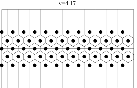
Figure 1: Regular structure with 5 rows at $\nu=4.17$, shown with its Voronoi construction for illustration purposes. This structure was obtained for 60 electrons in the unit cell.

III Numerical method

In order to find the ground state configuration of the system, the energy of the electrons in the parabolic confining potential is minimized with respect to the positions of the electrons for given confinement strength and density. As the number of particles used in the simulation is finite, commensurability effects are important. To realize a regular $M$-row structure, the number of particles in the simulation box has to be a multiple of $M$. Similarly, to realize a defected structure, the defect density is determined by the number of particles used in the simulation. To illustrate this, let us consider a five-row structure. Regular structures are realized for $N=5n$; for all other $N$, defects appear. As we expect the density to be maximal at the center and decrease towards the edges, the simplest symmetric defected structure possible is one where the outer rows are missing one particle each compared to the inner rows, i.e., structures of the form $[(n\!-\!1)nnn(n\!-\!1)]$. Such structures are realized for $N=5n-2$. The defect density may be defined as the number of missing particles in the outer rows divided by the number of particles in the inner rows, $n_{\rm def}=(n_{\rm inner}-n_{\rm outer})/n_{\rm inner}=1/n=5/(N+2)$. The minimum defect density that can be realized is, therefore, determined by the maximal number of particles that can be simulated. Thus, to find the ground state of the system, we have to vary $N$ at fixed confinement strength and density.

Conceptually, the proposed calculation is straightforward. The computational difficulty arises from the complexity of the minimization problem. It is well known from the study of related problems, e.g., the determination of the ground state of atomic clusters or the optimal arrangement of charges in a two-dimensional confined geometry gen_alg_1 ; gen_alg_2 ; gen_alg_3 , that the corresponding energy functional has a number of metastable states that increases exponentially with the number of particles. In such a case, classic minimization techniques are not the optimal choice.

Hybrid techniques employing genetic algorithms have been used in many related problems gen_alg_1 ; gen_alg_2 ; gen_alg_3 as a general tool to explore the available phase space more thoroughly and obtain better solutions with comparable computational cost to conventional optimization techniques. One frequently finds that counterintuitive disordered structures are favored.

For our case, a simulation box of finite length $L$ containing $N$ electrons is used. Periodic boundary conditions in the $x$-direction are enforced to remove size effects. For the summation of the interaction series, a quasi-one-dimensional restriction of the Ewald method is employed, following a similar technique to that reported in Ref. Ewald, . The appropriate methods of proven stability for our quasi-one-dimensional geometry are of complexity $O(N^{2})$ and this fact, in conjunction with the significant number of minimizations that need to be carried out (various system sizes for given total linear density), implies the necessity of substantial computational resources.

The total energy per particle of a particular configuration of $N$ electrons $\{r_{ij}\}$ can be written as

$$E\left[\{r_{ij}\}\right]=\frac{E_{0}}{N}\left\{\frac{r_{0}}{L}\varepsilon\left[\{r_{ij}\}\right]+\left(\frac{L}{r_{0}}\right)^{2}\sum_{ij}y_{ij}^{2}\right\},$$ (6)

where $E_{0}$ is the previously defined energy scale and distances are now measured in units of $L$. The complicated expression for the (dimensionless) interaction energy $\varepsilon$ and the details of its calculation are shown in appendix A. For a given number of electrons $N$ in a cell of length $L$, and a given density $\nu$, one has to minimize $E\left[\{r_{ij}\}\right]$ with respect to the electron configuration and thereby obtain the stable structure with energy $E_{\rm GS}(\nu;N)$.

In a nutshell, the algorithm proceeds along the following steps: An initial population of structures with random arrangements of electrons within the cell is partially relaxed towards a (local) minimum by a small number of iterations of a conventional minimization algorithm. Every member of the original population is then randomly split into two pieces, and the next generation is created by merging the pieces in all possible combinations while conserving the total number of particles. Subsequently, all newly obtained structures are fully relaxed to a (perhaps only local) minimum by a conventional minimization algorithm. A number of them is then chosen as parent structures for the next generation, always maintaining an appropriate diversity in the available configurations, i.e., a wide enough distribution in energies. The structure with the minimum energy is always retained to serve as a parent. The entire cycle is repeated until acceptable convergence is achieved. As expected, this hybrid approach is superior to simple minimization: it rapidly and consistently converges to complicated structures, avoiding being trapped in local minima.

In the end, to find the ground state configuration of the system at a given density $\nu$, the structure with the lowest energy, $E_{\rm GS}=\min_{N}\{E_{\rm GS}(\nu;N)\}$, is chosen.

IV Results

With the method described above, we are able to consider systems comprised of up to $N\sim 200$ electrons in the unit cell. We find that the lowest energy structures for a given energy are either regular structures, or structures where the linear density of the outer-most rows, $\nu_{\rm outer}$, is lower than the linear density of the inner rows, $\nu_{\rm inner}$ . The finite number of particles in the unit cell implies a lower limit to the defect density we can consider. Here we define the defect density as $n_{\rm def}=1-\nu_{\rm outer}/\nu_{\rm inner}$. For up to 6 rows, the number of particles per row exceeds 30. We are, therefore, able to identify defected structures with linear defect densities $n_{\rm def}$ down to $\sim 0.03$.

Let us summarize our main findings before discussing them in more detail: Up to 4 rows, the ground state of the system is free of defects. In the five-row structure, defects appear as one approaches the transition to 6 rows. Typical examples of such defected structures are shown in Fig. 2. We find that the defect density quickly increases with density and then levels off at values of the order $n_{\rm def}\sim 0.08$. Note that different types of defects appear: In the low density regime where the defect density rapidly increases with density, the structure possesses inversion symmetry with respect to $x$-axis, i.e., the centers of the defects in the two outer rows are located at the same $x$-position as shown in Fig. 2a. By contrast, the structures with the maximal defect density $n_{\rm def}\sim 0.08$ display defects that are maximally shifted with respect to each other along the $x$-direction as shown in Fig. 2b. The transition to six-row structures is shifted to a larger density as compared to the value given in Table 1. Above the transition, the ground state is a regular six-row structure. Only upon further increasing the density do defects appear again, before the transition to a seven-row structure. Further analyzing the spatial structure of the ground state configurations, we find that the presence of defects in the outer rows also affects the particle positions in the inner rows. While structures without defects consist of straight rows without corrugation, structures with defects display corrugation, i.e., distortions of the regular structure in both $x$- and $y$-direction.

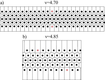
Figure 2: Defected structures with 5 rows at a) $\nu=4.70$ and b) $4.85$. The unit cell consists of 128 and 58 electrons, respectively, with the two outer rows missing an electron. The corresponding defect densities are $n_{\rm def}^{4.70}=1/26\approx 0.038$ and $n_{\rm def}^{4.85}=1/12\approx 0.083$. Electrons in red half-filled disks indicate the formal centers of the defects encountered.

IV.1 Defects in five- and six-row crystals

Using the full numerical minimization procedure, we find that the five-row Wigner crystal is stable in the density range $3.75<\nu<4.86$. Defected structures replace the regular ground state at $\nu_{c}^{(5)}=4.695$ and persist until the transition to 6 rows. Note that, as the finite number of particles limits the defect densities we can probe, the value $\nu_{c}^{(5)}$ represents an upper boundary for the range of stability of the regular structure.

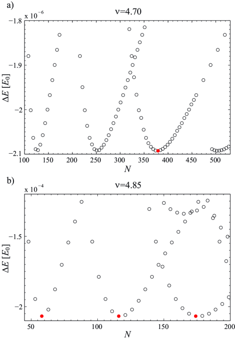
Figure 3: $E_{\rm GS}(N)$ at fixed density for a) $\nu=4.70$ and b) $\nu=4.85$. The energy is measured in units of $E_{0}=(e^{4}m\Omega^{2}/2\epsilon^{2})^{1/3}$ from the lowest-energy regular structure. a) For $\nu=4.70$, four minima can be clearly seen. As the defect densities sampled differ slightly, they are not exactly equal in energy. The global minimum is found at $N=379$, corresponding to a defect density $n_{\rm def}^{4.70}=0.390$. b) For $\nu=4.85$, three degenerate minima appear at $N=58,116,174$, all corresponding to a defect density of $n_{\rm def}^{4.85}=0.083$.

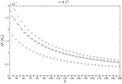
Figure 4: Difference in energy at fixed density $\nu=4.17$ as a function of the size of the unit cell. $N=5n-1$ structures [$(n\!-\!1)nnnn$] form the lowest excitation branch, followed by $N=5n+1$ [$n(n\!+\!1)nnn$], $N=5n-2$ [$(n\!-\!1)nnn(n\!-\!1)$], and $N=5n-3$ [$(n\!-\!1)(n\!-\!1)nn(n\!-\!1)$]. Fitting the lowest excitation branch to a general functional form $\alpha+\beta/N^{\gamma}$ we obtain $\gamma\sim 1$ and an energy gap in the thermodynamic limit $\Delta E_{\infty}=2\times 10^{-7}$.

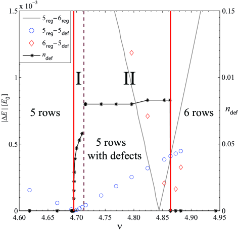
Figure 5: Energy gaps $|\Delta E|$ and boundaries for the various phases encountered. The red vertical lines show the phase boundaries as obtained by the location of the zero of the corresponding energy difference between: five-row regular and five-row defected structures (blue circles), six-row regular and five-row defected structures (red rhombi). The dashed line indicates the location of a first order transition between the two types of defects encountered: in region I the centers of the defects coincide whereas in region II the centers of the defects are maximally separated within the unit cell. The grey line shows the energy difference between five- and six-row regular structures. (Its zero is the prediction for the phase boundary under the assumption of regular rows.) Furthermore, the black stars show the defect density $n_{\rm def}$ as a function of density $\nu$. Note the jump at the boundary between regions I and II.

A regular five-row crystal is shown in Fig. 1 whereas two defected five-row crystals are shown in Fig. 2. The five-row crystals in Fig. 2 correspond to $\nu=4.70$ and $\nu=4.85$, and have a defect density $n_{\rm def}=0.038$ and $n_{\rm def}=0.083$, respectively. Fig. 3 shows how the defected structures were identified. In particular, the ground state energy at fixed density $\nu=4.85$ as a function of the number of particles in the unit cell is shown. Regular five-row structures are realized for $N=5n$ with $n\in\mathbb{N}$. For all other $N$, defected structures are obtained. Let us discuss the high density structure $\nu=4.85$ displayed in Fig. 3b first. Three equivalent minima at $N=58$, $N=116$, and $N=174$ can be clearly seen. These minima correspond to configurations with defects in the outer-most rows, i.e., the outer rows have less particles than the inner rows, namely $N_{\rm inner}=12\;(24,36)$, and $N_{\rm outer}=11\;(22,33)$, respectively. The corresponding defect density is $n_{\rm def}^{4.85}=1-11/12=0.083$. The low-energy structure $\nu=4.70$ displayed in Fig. 3a displays only one minimum at $N=128$ within the regime that can be explored by the full minimization procedure. This minimum corresponds to a defect density $\tilde{n}_{\rm def}^{4.70}=0.0385$. To rule out finite size effects, we extended our calculation to a larger number of particles employing conventional minimization techniques, utilizing as starting guesses the structures obtained form the full minimization in the smaller unit cell. As Fig. 3a shows, further minima appear at $N=251$, $N=379$, and $N=502$ corresponding to approximately the same defect density. In fact, the lowest energy structure is obtained for $N=379$ where $n_{\rm def}^{4.70}=0.0390$.

For comparison, Fig. 4 shows the equivalent diagram at a lower fixed density $\nu=4.17$ corresponding to the regular ground state shown in Fig. 1. The energy of defected structures keeps decreasing with defect density until the lowest defect density $n_{\rm def}=1-39/40=0.025$ reached given our limitation on the number of particles. Note that the lowest excitation branch shown in the picture corresponds to structures missing one particle from only one of the outer rows. Fitting that branch to a general functional form $\alpha+\beta/N^{\gamma}$ we obtain $\gamma\sim 1$ and an energy gap in the thermodynamic limit $\Delta E_{\infty}=2\times 10^{-7}$. Thus, we do not expect that the regular structure becomes unstable at even lower defect densities.

Our findings in the vicinity of the transition from 5 to 6 rows are summarized in Fig. 5. The defect density as well as the energy gaps to the lowest-lying regular or defected structure are shown as a function of density. Note that due to the substantial computational effort involved, the density interval is not uniformly sampled. As mentioned earlier, the defect density quickly increases in a narrow density interval and then levels off to an almost constant value until the transition to six rows is reached. The six-row crystal is stable in the density range $4.86<\nu<6.04$. It develops defects at around $\nu=5.75$, which also persist until the transition to 7 rows.

To better understand the structures that appear we now turn to a more detailed analysis of the spatial arrangement of particles in the crystal.

IV.2 Analysis of row corrugation

As can be seen from Fig. 2, two types of defected structures appear. These two structures can be distinguished by analyzing the distortion of the crystal. The distances between rows vary as a function of density. While regular structures consist of straight rows, structures with defects display corrugation. Let us label the positions of particles as ${\bf r}_{j}^{(k)}$, where $j$ denotes the row and $k$ denotes the position along the row. In regular structures, we find $y_{j}^{(k)}=y_{j}^{(k^{\prime})}$ for all $j,k,k^{\prime}$, within the accuracy of the calculation. For the defected structures, we define the average displacement of each row

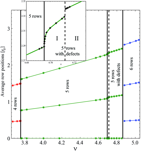
Figure 6: Average positions of the crystal rows in units of $r_{0}$ as a function of density. Note that due to symmetry, only half of the rows are shown. The inset shows the detailed behavior at the transition from the regular five-row to the defected five-row structure. For regular structures, the distance between rows increases linearly with $\nu$. In region I, the distance between rows increases more rapidly. At the boundary between regions I and II, there is a jump. In region II, the distance increases again linearly with the same slope as for the regular structures.

$$\overline{y}_{j} = \sum_{k=1}^{N_{j}}y_{j}^{(k)}/N_{j},$$ (7)

where $N_{j}$ is the number of particles in row $j$. In Fig. 6, the average positions of the rows are shown. Due to the symmetry of the structure only half of them are displayed.

As expected, there are jumps at the transition to a structure with a larger number of rows; in the intermediate region the distance grows linearly with density. Interestingly, as shown in the inset, a continuous transition to the structures with defects appears to take place. The transition also marks the onset of corrugation in the crystal structure. However, within the density regime of defected structures, we find a discontinuity. In the region labeled I, the distance between rows increases rapidly, a behavior that is well fitted by a square root. At the boundary between regions I and II, the row position displays a jump before it increases linearly again in region II. This suggests two different defected phases that can be characterized by their corrugation.

A close look at the defected structure reveals that the corrugation exists in both directions, along and perpendicular to the wire axis. We define the corrugation in the $y$-direction as the deviation from the average row position in that direction,

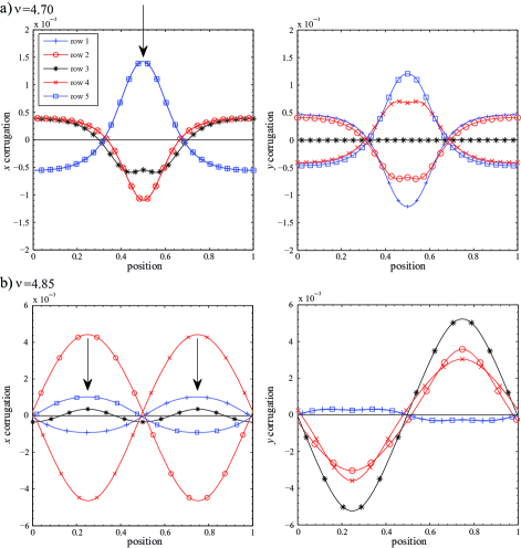
Figure 7: Corrugation in the transverse (right panels) and longitudinal (left panels) direction for the defected structures that appear at a) $\nu=4.70$ (top panels) and b) $\nu=4.85$ (bottom panels). For the definition of the corresponding quantities please see the main text. The corrugation in the longitudinal direction (left) is measured in units of the average inter-particle distance within the row, while that in the transverse direction (right) is measured in units of the average distance between rows. The arrows indicate the particle located at the center of the defect in each case. See also Fig. 2.

$$\delta y_{j}^{(k)} = y_{j}^{(k)}-\overline{y}_{j}.$$ (8)

We can also define the average inter-particle distance for a given row $j$ by

$$\overline{\Delta x}_{j} = \sum_{k=1}^{N_{j}}(x_{j}^{(k+1)}-x_{j}^{(k)})/N_{j}=\nu_{j}^{-1},$$ (9)

where $\nu_{j}$ is the dimensionless density in that row. Note that $\nu=\sum_{n=1}^{M}\nu_{j}$. Subsequently, we define the corrugation in the $x$-direction by

$$\delta(\Delta x)_{j}^{(k+1\,k)} = x_{j}^{(k+1)}-x_{j}^{(k)}-\overline{\Delta x}_{j}.$$ (10)

While the corrugation is less than one percent in both directions, it turns out to be very important in determining the ground state of the system. Figure 7 shows examples of the two dominant types of corrugation accompanying five-row defected structures. Note that the arrows indicate the particle located at the center of the defect in each case. As before, the chosen density values are $\nu=4.70$ and $\nu=4.85$, close to the boundaries shown in Figs. 5 and 6. Fig. 7a shows the corrugation for $\nu=4.70$, i.e., a structure close to the density where defects first appear. This kind of corrugation is typical for the narrow density regime $4.695<\nu<4.712$, where the defect density rapidly increases with $\nu$. Fig. 7b shows the corrugation for $\nu=4.85$ with defect density $n_{\rm def}=0.083$. This kind of corrugation is characteristic of the structures exhibiting the maximum defect density $n_{\rm def}\sim 0.08$.

Qualitatively, the two types of structures exhibit different features. In the first defected structure that is encountered, see Fig. 7a, the defects in the exterior rows are rather localized, and they are located at the same position along the crystal. The displacements are maximal for the outer rows and decrease as one moves towards the interior of the crystal. In particular, due to the symmetry of the defect, the innermost row exhibits no corrugation in the $y$-direction at all. At higher density, both the $x$- and $y$-corrugations are approximately sinusoidal. Furthermore, the defects on the two exterior rows are maximally separated, i.e., they are shifted by half a period, see Fig. 7b. For this kind of structures, the center line possesses the maximum amplitude of $y$-oscillations. A possible explanation is that, while the interaction energy (which drives the corrugation) is only sensitive to the relative corrugation, a deformation of the inner rows entails a smaller change in confining potential energy.

We, thus, encounter two distinct phases with defects. Fig. 8a shows the energy as a function of defect density for different densities close to the boundary between the two phases. Two minima corresponding to the different types of defected structures can be clearly identified. The position of one of the minima changes rapidly with density. This minimum corresponds to the type of defect encountered in the low-density regime. The position of the other minimum barely shifts with density. This minimum corresponds to the sinusoidal defects encountered in the high-density regime. At low density, it describes a metastable state. However, its energy with respect to the other minimum decreases with density until, at $\nu_{\rm I-II}^{(5)}=4.712$, it eventually becomes the global minimum and, therefore, the ground state. Both the defect density (Fig. 5) and the distance between rows (Fig. 6) display a discontinuity at the transition. The transition between the two defected phases is, thus, of first order.

The nature of the transition from regular to defected structures is more difficult to identify as it requires going to very low defect densities. The fact, that with decreasing density, the defect density becomes lower and lower, until we reach the minimal value we can simulate, suggests, however, that the transition might be second order. In order to approach this transition, simplified models that allow one to simulate a larger number of particles are required. This models, then, may also be used in order to extend the calculation to larger number of rows.

V Simplified minimization procedures

The full minimization procedure is computationally intensive which sets practical limits on the size of the unit cell one can simulate. That in turn imposes constraints on the defect density. Therefore, simplified models that allow us to simulate a larger number of particles are worth investigating to gain a better understanding. We start with the simplest model possible, compare with the results of the full simulation described above, and then discuss possible improvements.

Up to six rows, we find that defected structures have less particles in the outer rows. In the previous section, we pointed out that these defected structures display corrugation. As a first approximation, one may neglect this corrugation and assume that all rows are straight and regular, i.e., $\delta y_{j}^{(k)}=\delta(\Delta x)_{j}^{(k+1\;k)}=0$. Defects are incorporated by allowing the linear densities in the inner and outer rows to differ–in particular, the two outer rows have less particles, $n_{\rm outer}<n_{\rm inner}$. The density of defects is controlled by the parameter $\lambda=n_{\rm inner}/n_{\rm outer}$, i.e., the density of defects is then given as $n_{\rm def}=1-\lambda^{-1}$. In that case, for a fixed defect density, one has a minimization involving $2M-1$ parameters, namely the $y$-position of the rows and their relative shifts in the $x$-direction. Assuming that defects are located in the outer rows, the calculation can be further improved by “unfreezing” the $x$-positions of particles in the outer rows. This is the method we will use in the following. Given the much reduced parameter space, a conventional minimization procedure is sufficient here.

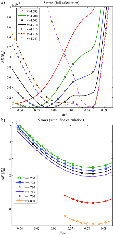
Figure 8: a) Difference $\Delta E=E_{\rm defect}-E_{\rm regular}$ for five-row structures as a function of defect density $n_{\rm def}$ within a simplified calculation scheme that incorporates defects by allowing the linear densities in the inner and outer rows to be different. Note that there is a region before the critical $\nu=4.86$ of the $5\rightarrow 6$ transition where the defected structures become stable. b) Energy of five-row defected structures at various densities as a function of defect density $n_{\rm def}$ using the full minimization procedure. The minima are shifted to zero for clarity of presentation. Note that the minimum present at small defect densities is not captured by the simplified method.

The findings for five-row structures are shown in Fig. 8a. Note that the model captures correctly the appearance of defects in the five-row structure, and it also predicts a regular ground state for the four-row crystal. Furthermore, the maximal defect density is reproduced: For the five-row structure, we can see that the defect density $n_{\rm def}\sim 0.08$ leading to the minimal energy is in agreement with the full minimization.

Analyzing the results in more detail, (expected) discrepancies are found. Due to the constraints imposed, the energies of defected structures are too high. For the five-row structures for example, the simplified model finds that defects appear around $\nu=4.78$ whereas the full minimization reveals that defected structures become the ground state configuration already at a lower density $\nu=4.695$. Furthermore, the simplified model does not capture the rise in defect density up to the maximal value. In particular, the simplified model completely misses the low-density regime with symmetric defects. Comparing Figs. 8a and b, the additional minimum at low-defect densities present in Fig. 8a is clearly absent in Fig. 8b. Thus, the simplified method only captures the high-density phase with sinusoidal defects. The reason is most likely that it corresponds to a fairly smooth corrugation and, therefore, is still present when one imposes straight rows. By contrast, the minimum at low defect densities is associated with fairly sharp features in the corrugation profile and may, therefore, be suppressed by imposing straight regular rows. In particular, it is straightforward to verify that, for constant linear density in the inner rows, the defects on the outer rows will be maximally separated. In order to obtain a defected structure where the centers of the defects coincide, a longitudinal distortion of the inner rows is indispensable.

To summarize, the simplified model correctly reproduces the typical defect density–though it overestimates the energy of the defected structures which therefore are stable only in a reduced density interval. However, the model does not reproduce the low-density defected phase and, therefore, can not be used to explore the nature of the transition from regular to defected structures. The method may be used to study the stability of regular structures for structures with more rows. We find that upon further increasing the number of rows, the regime of densities where the ground state contains defects widens. Under the assumption that only the outer rows contain defects, regular structures disappear completely once the number of rows exceeds nine, as is evident from table 2. As the simplified method overestimates the energy of defected structures and misses the phase with symmetric defects, it is likely that regular crystals cease to be the ground state already for a smaller number of rows.

As is also shown in Table 2, the typical defect density increases with the number of rows and also slightly varies with density for a given number of rows. Note that considering structures of the type $[(n\!-1\!)n\dots n(n\!-1\!)]$, the defect densities obtained can only take the discrete values $n_{\rm def}=1/n$.

Table 2: Number of rows and defect density in the crystal as a function of the dimensionless density $\nu$. All numbers shown were obtained using the simplified minimization procedure described in Sec. V.

# of	total	density range	$n_{\rm def}$
rows	density range	with defects
4	$2.72<\nu<3.75$	N/A	N/A
5	$3.75<\nu<4.86$	$4.77<\nu<4.86$	0.083
6	$4.86<\nu<6.04$	$5.75<\nu<6.04$	0.091–0.100
7	$6.04<\nu<7.31$	$6.76<\nu<7.31$	0.100–0.111
8	$7.31<\nu<8.64$	$7.80<\nu<8.64$	0.100–0.125
9	$8.64<\nu<10.01$	$8.87<\nu<10.01$	0.111–0.125
10	$10.01<\nu<11.37$	$10.01<\nu<11.37$	0.125–0.143
11	$11.37<\nu<12.77$	$11.37<\nu<12.77$	0.125–0.143
12	$12.77<\nu<14.19$	$12.77<\nu<14.19$	0.143–0.167
13	$14.19<\nu<15.67$	$14.19<\nu<15.67$	0.143–0.167

Eventually, one expects that more complicated structures will appear. The simple configuration we studied is in competition with structures where defects appear away from the edges, such as structures of the type $[(n\!-\!1)(n\!-\!1)n\dots n(n\!-\!1)(n\!-\!1)]$, for example. Detailed calculations within these simplified models reveal that such structures are indeed competitors for the ground state, but up to 13 rows such a minimum is not realized.

To approach the transition between regular and defected rows, we use a different trick. An unbiased search for the global minimum is numerically costly because a simple minimization may get stuck in a metastable minimum. However, if the initial guess of the electron configuration is sufficiently close to the global minimum, a simple minimization will converge. Having identified the structure of defects in region I, one may feed such structures into a simple minimization at lower densities. The results of such a procedure have been included in Figs. 5 and 6. There, structures with defect densities down to $n_{\rm def}\sim 0.03$ were obtained with the full minimization, whereas structures close to the phase boundary with lower defect structures were obtained with the method described here. The results suggest that the defect density indeed vanishes at the transition which points to a second order phase transition.

VI Conclusion

We study quasi-one-dimensional systems of classical particles interacting via long-range Coulomb interactions and confined by a parabolic potential in the transverse direction. The ground state configurations are multi-row Wigner crystals where the number of rows is controlled by the density (or the strength of the confining potential). We find that defects that accommodate the density variation in the transverse direction appear once the number of rows exceeds four.

Defected structures have less particles in the outer than in the inner rows. The full numerical minimization for five rows reveals that two distinct types of defected phases exist. Upon increasing density, the regular structure at low-densities is replaced by a structure with symmetric defects, i.e., where the center of the defect on the two outer rows is located at the same $x$-position. As the number of particles that can be simulated sets a lower limit on the defect density that can obtained, the full minimization allows one only to provide an upper limit for the density at the transition from regular to defected structures. We extend our calculations to lower densities by using structures with the type of defect described above as the input for a simple minimization. The results indicate that the defect density vanishes at $\nu_{c}^{(5)}=4.695$ and that the transition is of second order. To obtain symmetric defects, the longitudinal distortion of the inner rows, namely an increased density at the center of the defect, is crucial. Any analytical description of the transition would have to take into account this distortion.

Upon further increasing density, the defect density rapidly increases. At a critical density, $\nu_{\rm I-II}^{(5)}=4.712$, structures with a different type of defect corresponding to a sinusoidal distortion of the rows with a phase shift of half a period between the two outer rows become become the ground state. This second regime is characterized by a defect density that barely varies with density and extends up to the transition to six rows. The transition between the two defected phases with different symmetries is first order.

Simplified models neglecting the corrugation of the rows only capture this second defected phase. Thus, these models do not allow one to further investigate the nature of the phase transition from regular to defected structures. However, as this second phase occupies most of the density interval, they may be used to study the stability of regular structures upon increasing the number of rows. We find that beyond nine rows, no stable regular structures exist. Taking into account that the simplified model overestimates the energy of defected structures, we expect that stable regular structures may disappear even earlier.

Appendix A Ewald summation method for a quasi-one-dimensional geometry

The method we use essentially follows the steps outlined in Ref. Ewald, . It is based on the Poisson summation formula relating summations over direct and reciprocal space,

$$\sum_{n=-\infty}^{+\infty}f(nL)=\frac{1}{L}\sum_{m=-\infty}^{+\infty}F\left(\frac{2\pi m}{L}\right),$$ (11)

where the Fourier transform of $f(x)$ is defined as

$$F(k)=\int_{-\infty}^{+\infty}\!\!\!\mathrm{d}x\,e^{ikx}f(x).$$ (12)

Let us consider the function $f(x)=e^{-(\rho+x)^{2}t}$. By completing the square and carrying out the Fourier transform integration, we obtain the fundamental equation

$$\sum_{n=-\infty}^{+\infty}e^{-(\rho+nL)^{2}t}=\frac{\sqrt{\pi}}{L}t^{-1/2}\sum_{G}e^{iG\rho}e^{-\frac{G^{2}}{4t}},$$ (13)

where the reciprocal lattice vectors are given by $G=2\pi m/L$ with $m=0,\pm 1,\dots$. The following definition of the incomplete $\Gamma$ function is extensively used and therefore given here for reference:

$$\frac{\Gamma({\mu,ux^{2}})}{x^{2\mu}}=\int_{u}^{+\infty}\!\!\!\mathrm{d}t\,t^{\mu-1}e^{-x^{2}t}.$$ (14)

The system we are considering contains a basic cell of length $L$ with $N$ electrons. The spatial extent in the $y$-direction is limited by the confining potential. In the $x$-direction, we impose periodic replications of the basic cell to avoid edge effects. The interaction energy per cell of the system can be written

$$\tilde{\epsilon}[\{{\bf r}_{ij}\}]=\frac{1}{2}\sum_{i\neq j}\sum_{n}\frac{q_{i}q_{j}}{|{{\bf r}}_{ij}+nL\hat{{\bf x}}|}+\frac{1}{2}\sum_{j}q_{j}^{2}\sum_{n\neq 0}\frac{1}{|nL\hat{\bf x}|},$$ (15)

where $q_{i}$ is the charge of particle $i$, ${\bf r}_{ij}={\bf r}_{i}-{\bf r}_{j}$, and the index $n$ runs over replicas of the unit cell. The artificial separation of the terms is for our convenience. We then introduce the notation

$$\Phi({\bf r}) =\sum_{n}\frac{1}{|{\bf r}+nL\hat{\bf x}|}$$ (16)

for $|{\bf r}|\neq 0$ and $\Phi_{0}=\sum_{n\neq 0}\displaystyle{1/|nL\hat{\bf x}|}$.

In what follows we will split the summations in direct and reciprocal space. To cancel the divergencies appearing in the above sums, we will assume a uniform neutralizing background charge.

Using Eq. (14), we obtain the following representation,

$$\Phi({\bf r}) =\frac{1}{\sqrt{\pi}}\sum_{n}\int_{0}^{+\infty}\!\!\!\mathrm{d}t\,t^{-1/2}e^{-|{\bf r}+nL\hat{\bf x}|^{2}t}.$$ (17)

Here we will introduce an artificial separation constant $\alpha$ which will control the splitting of the summation between direct and reciprocal space. We then have $\Phi({\bf r})=\Phi^{>}({\bf r})+\Phi^{<}({\bf r})$, where

$$\Phi^{>}({\bf r}) =\frac{1}{\sqrt{\pi}}\sum_{n}\int_{\alpha^{2}}^{+\infty}\!\!\!\mathrm{d}t\,t^{-1/2}e^{-|{\bf r}+nL\hat{\bf x}|^{2}t}$$

$$=\sum_{n}\frac{\mathrm{erfc}(\alpha|{\bf r}+nL\hat{\bf x}|)}{|{\bf r}+nL\hat{\bf x}|}$$ (18)

and

$$\Phi^{<}({\bf r}) =\frac{1}{\sqrt{\pi}}\sum_{n}\int_{0}^{\alpha^{2}}\!\!\!\mathrm{d}t\,t^{-1/2}e^{-(x+nL)^{2}t}e^{-y^{2}t}.$$ (19)

To evaluate $\Phi^{<}({\bf r})$, we use Eq. (13) yielding

$$\Phi^{<}({\bf r}) =\frac{1}{L}\sum_{G}e^{iGx}\int_{0}^{\alpha^{2}}\!\!\!\mathrm{d}t\,t^{-1}e^{-\frac{G^{2}}{4t}}e^{-y^{2}t}.$$ (20)

While for $G\neq 0$ the integration yields incomplete Bessel functions ,

$$\int_{0}^{\alpha^{2}}\!\!\!\mathrm{d}t\,t^{-1}e^{-\frac{G^{2}}{4t}}e^{-y^{2}t}=K_{0}\left(\frac{G^{2}}{4\alpha^{2}},\alpha^{2}y^{2}\right),$$ (21)

the $G=0$ term (denoted $I_{0}$ in the following) is divergent and has to be treated separately. Using the substitution $z=\alpha^{2}/t$ and expanding the second exponential, one finds

$$I_{0} =\frac{1}{L}\lim_{G\rightarrow 0}\int_{1}^{+\infty}\!\!\!\mathrm{d}z\,z^{-1}e^{-\frac{G^{2}}{4\alpha^{2}}z}\sum_{m=0}^{+\infty}\frac{(-1)^{m}}{m!}(\alpha y)^{2m}z^{-m}.$$

The divergent contribution comes from $m=0$, namely

$$\lim_{G\rightarrow 0}\int_{1}^{+\infty}\!\!\!\mathrm{d}z\,z^{-1}e^{-\frac{G^{2}}{4\alpha^{2}}z} = -\gamma+\ln 4\alpha^{2}-\lim_{G\rightarrow 0}\ln G^{2}.$$

The rest of the sum can be evaluated to

$$\sum_{m=1}^{+\infty}\int_{1}^{+\infty}\!\!\!\mathrm{d}z\,z^{-1}\frac{(-1)^{m}}{m!}(\alpha y)^{2m}z^{-m}$$

$$= \sum_{m=1}^{+\infty}\frac{(-1)^{m}}{mm!}(\alpha y)^{2m}=-\gamma-\ln(\alpha^{2}y^{2})-\Gamma(0,\alpha^{2}y^{2}).$$

Thus,

$$I_{0} =-\frac{1}{L}\left\{2\gamma+\lim_{G\rightarrow 0}\ln G^{2}+\ln(y^{2}/4)+\Gamma\left(0,\alpha^{2}y^{2}\right)\right\},$$

and

$$\Phi^{<}({\bf r}) = \frac{1}{L}\sum_{G\neq 0}e^{iGx}K_{0}\left(\frac{G^{2}}{4\alpha^{2}},\alpha^{2}y^{2}\right)+I_{0}.$$ (23)

Splitting up $\Phi_{0}$ in the same way, we find

$$\Phi_{0}^{>}({\bf r}) =\sum_{n\neq 0}\frac{\mathrm{erfc}(\alpha|n|L)}{|n|L}$$ (24)

and

$$\Phi_{0}^{<}({\bf r}) = \frac{1}{L}\sum_{G}\int_{0}^{\alpha^{2}}\!\!\!\mathrm{d}t\,t^{-1}e^{-\frac{G^{2}}{4t}}-\frac{1}{\sqrt{\pi}}\int_{0}^{\alpha^{2}}\!\!\!\mathrm{d}t\,t^{-1/2}$$

$$= \frac{1}{L}\sum_{G\neq 0}\Gamma\left(0,\frac{G^{2}}{4\alpha^{2}}\right)$$

$$-\frac{1}{L}\left\{\gamma-\ln 4\alpha^{2}+\lim_{G\rightarrow 0}\ln G^{2}\right\}-\frac{2\alpha}{\sqrt{\pi}}.$$

At this stage we put everything together, $\tilde{\epsilon}[\{{\bf r}_{ij}\}]=\frac{1}{2}\sum_{i\neq j}q_{i}q_{j}\Phi({\bf r}_{ij})+\frac{1}{2}q_{j}^{2}\Phi_{0}$, and combining various terms we obtain the result for the interaction energy per cell of the system,

$$\tilde{\epsilon}[\{{\bf r}_{ij}\}] = \frac{1}{2}\sum_{i,j}q_{i}q_{j}\left\{{\sum_{n}}^{\prime}\frac{\mathrm{erfc}(\alpha|{\bf r}_{ij}+nL\hat{\bf x}|)}{|{\bf r}_{ij}+nL\hat{\bf x}|}+\frac{1}{L}\sum_{G\neq 0}e^{iGx_{ij}}K_{0}\left(\frac{G^{2}}{4\alpha^{2}},\alpha^{2}y_{ij}^{2}\right)\right\}$$

$$-\frac{1}{2L}\sum_{i\neq j}q_{i}q_{j}\left[\gamma+\ln{\alpha^{2}y^{2}_{ij}}+\Gamma(0,\alpha^{2}y^{2}_{ij})\right]-\frac{\alpha}{\sqrt{\pi}}\sum_{j}q_{j}^{2}-\frac{1}{2L}\left(\sum_{j}q_{j}\right)^{2}\left[\gamma-\ln 4\alpha^{2}+\lim_{G\rightarrow 0}\ln G^{2}\right],$$

where the notation ${\sum_{n}}^{\prime}$ implies that for $n=0$ there is no self-interaction term in the summation. For a charge neutral system, the last term vanishes. For a system of electrons, as the one under consideration, a uniform positive neutralizing background will exactly cancel the divergent term $\lim_{G\rightarrow 0}\ln G^{2}$.

We define a dimensionless separation constant through $\alpha=\widetilde{\alpha}/L$ and introduce dimensionless coordinates. Subsequently, the dimensionless interaction energy per electron in the simulation box can be cast as follows

$$\varepsilon[\{{\bf r}_{ij}\}]=\frac{1}{2}\sum_{i,j}f[\{{\bf r}_{ij}\}]-\frac{N\widetilde{\alpha}}{\sqrt{\pi}}-N^{2}\left[\gamma-\ln{\left(\frac{2\widetilde{\alpha}}{L}\right)}\right],$$

with

$$f[\{{\bf r}_{ij}\}] = {\sum_{n}}^{\prime}\frac{\mathrm{erfc}\left(\widetilde{\alpha}\sqrt{(x_{ij}+n)^{2}+y_{ij}^{2}}\right)}{\sqrt{(x_{ij}+n)^{2}+y_{ij}^{2}}}+2\sum_{q=1}^{+\infty}\cos\left(2\pi qx_{ij}\right)K_{0}\left(\frac{\pi^{2}q^{2}}{\widetilde{\alpha}^{2}},\widetilde{\alpha}^{2}y_{ij}^{2}\right)-\ln\widetilde{\alpha}^{2}y_{ij}^{2}-\Gamma(0,\widetilde{\alpha}^{2}y_{ij}^{2}).$$ (28)

References

- (1) E. Wigner, Phys. Rev. 46, 1002 (1934).
- (2) P. Glasson, V. Dotsenko, P. Fozooni, M. J. Lea, W. Bailey, G. Papageorgiou, S. E. Andresen, and A. Kristensen, Phys. Rev. Lett. 87, 176802 (2001).
- (3) E. Rousseau, D. Ponarin, L. Hristakos, O. Avenel, E. Varoquaux, and Y. Mukharsky, Phys. Rev. B 79, 045406 (2009).
- (4) Yu. Z. Kovdrya, Low Temp. Phys. 29, 77 (2003).
- (5) H. Ikegami, H. Akimoto, and K. Kono, Phys. Rev. B 82, 201104 (2010).
- (6) K. A. Matveev, Phys. Rev. Lett. 92, 106801 (2004); Phys. Rev. B 70, 245319 (2004); A. D. Klironomos, R. R. Ramazashvili, and K. A. Matveev Phys. Rev. B 72, 195343 (2005).
- (7) G. Piacente, I. V. Schweigert, J. J. Betouras, and F. M. Peeters, Phys. Rev. B 69, 045324 (2004).
- (8) A. D. Klironomos, J. S. Meyer, and K. A. Matveev, Europhys. Lett. 74 679 (2006); A. D. Klironomos, J. S. Meyer, T. Hikihara, and K. A. Matveev, Phys. Rev B 76, 75302 (2007).
- (9) S. Akhanjee and J. Rudnick, Phys. Rev. Lett 99, 236403 (2007).
- (10) G. A. Fiete, Rev. Mod. Phys. 79, 801 (2007).
- (11) J. S. Meyer, K. A. Matveev, and A. I. Larkin, Phys. Rev. Lett. 98, 126404 (2007).
- (12) V. V. Deshpande and M. Bockrath, Nature Physics 4, 314 (2008).
- (13) D. Hughes and P. Ballone, Phys. Rev. B 77, 245312 (2008).
- (14) L. Shulenburger, M. Casula, G. Senatore, and R. M. Martin, Phys. Rev. B 78, 165303 (2008).
- (15) W. K. Hew, K. J. Thomas, M. Pepper, I. Farrer, D. Anderson, G. A. C. Jones, and D. A. Ritchie, Phys. Rev. Lett. 102, 056804 (2009).
- (16) Y. Tserkovnyak and M. Kindermann, Phys. Rev. Lett. 102, 126801 (2009).
- (17) L. W. Smith, W. K. Hew, K. J. Thomas, M. Pepper, I. Farrer, D. Anderson, G. A. C. Jones, and D. A. Ritchie, Phys. Rev. B 80, 041306 (2009).
- (18) S. A. Soffing, M. Bortz, I. Schneider, A. Struck, M. Fleischhauer, and S. Eggert, Phys. Rev. B 79, 195114 (2009).
- (19) G. Piacente, G. Q. Hai, and F. M. Peeters, Phys. Rev. B 81, 024108 (2010).
- (20) K. A. Matveev, A. V. Andreev, and M. Pustilnik, Phys. Rev. Lett. 105, 046401 (2010).
- (21) R. Cortes-Huerto, M. Paternostro, and P. Ballone, Phys. Rev. A 82, 013623 (2010).
- (22) L. H. Kristinsdóttir, J. C. Cremon, H. A. Nilsson, H. Q. Xu, L. Samuelson, H. Linke, A. Wacker, and S. M. Reimann, Phys. Rev. B 83, 041101 (2011).
- (23) J. S. Meyer and K. A. Matveev, J. Phys.: Condens. Matter 21, 23203 (2009).
- (24) V. V. Deshpande, M. Bockrath, L. I. Glazman, and A. Yacoby, Nature 464, 7286 (2010).
- (25) A. V. Chaplik, Pisma Zh. Eksp. Teor. Fiz. 31, 275 (1980) [JETP Lett. 31, 252 (1980)].
- (26) R. W. Hasse and J. P. Schiffer, Ann. Phys. 203, 419 (1990).
- (27) G. Birkl, S. Kassner, and H. Walther, Nature 357, 310 (1992).
- (28) I. A. Larkin and V. B. Shikin, Phys. Lett. A 151, 335 (1990).
- (29) D. B. Chklovskii, K. A. Matveev, and B. I. Shklovskii, Phys. Rev. B 47, 12605 (1993).
- (30) A. A. Koulakov and B. I. Shklovskii, Phys. Rev. B 57, 2352 (1998).
- (31) J. R. Morris, D. M. Deaven, and K. M. Ho, Phys. Rev. B 53, R1740 (1996).
- (32) K. Michaelian, N. Rendón, and I. L. Garzón, Phys. Rev. B 60, 2000 (1999).
- (33) M. Porto, J. Phys. A: Math. Gen. 33, 6211 (2000).
- (34) F. E. Harris and J. G. Fripiat, Int. J. Quantum Chem. 109, 1728 (2009).