Quasiclassical description of a superconductor with a spin density wave

Abstract

We derive equations for the quasiclassical Green’s functions $\check{g}$ within a simple model of a two-band superconductor with a spin-density-wave (SDW). The elements of the matrix $\check{g}$ are the retarded, advanced, and Keldysh functions each of which is an $8\times 8$ matrix in the Gor’kov-Nambu, the spin and the band space. In equilibrium, these equations are a generalization of the Eilenberger equation. On the basis of the derived equations we analyze the Knight shift, the proximity and the dc Josephson effects in the superconductors under consideration. The Knight shift is shown to depend on the orientation of the external magnetic field with respect to the direction of the vector of the magnetization of the SDW. The proximity effect is analyzed for an interface between a superconductor with the SDW and a normal metal. The function describing both superconducting and magnetic correlations is shown to penetrate the normal metal or a metal with the SDW due to the proximity effect. The dc Josephson current in an $S_{SDW}/N/S_{SDW}$ junction is also calculated as a function of the phase difference $\varphi$. It is shown that in our model the Josephson current does not depend on the mutual orientation of the magnetic moments in the superconductors $S_{SDW}$ and is proportional to $\sin\varphi$. The dissipationless spin current $j_{sp}$ depends on the angle $\alpha$ between the magnetization vectors in the same way ($j_{sp}\sim\sin\alpha$) and is not zero above the superconducting transition temperature.

I Introduction

Coexistence of two or more order parameters in solids is one of the most intriguing phenomena in condensed matter physics. There are many systems where the ordered phases are even antagonistic to each other. Nowadays, a very popular subject of research are compounds with coexisting superconducting (SC) and magnetic (M) order parameters.

It is already well known, that the exchange field responsible for ferromagnetism destroys singlet Cooper pairs BuzdinRMP but can generate BVErmp ; Eschrig triplet ones (odd in frequency and symmetric in space) that survives even in the presence of a strong exchange field and strong impurity scattering. The theoretical prediction has been recently confirmed experimentally Klapwijk ; Sosnin ; Birge ; Robinson ; Westerholt ; Aarts .

In contrast, a magnetic order of the antiferromagnetic type can coexist with singlet Cooper pairs because the average magnetic moment (on distances of order of the size of the Cooper pairs) is close to zero. This case is realized in superconductors with a spiral magnetic structure (for a review, see BulaevRev and references therein).

Another example of this coexistence are superconductors with a spin-density wave (SDW) Tugushev ; Kopaev ; Littlewood . This type of superconductivity coexisting with the SDW is realized in quasi-one-dimensional conductors (for a review, see Chaikin ). A lot of attention is payed now to quasi-two-dimensional superconducting compounds – the so-called Fe-based pnictides – discovered recently Discov1 ; Discov2 ; Discov3 ; Discov4 . Some of these Fe-based superconductors have rather high critical temperature $T_{c}$ of the superconducting transition (up to 56 K observed in $Gd_{1-x}Th_{x}FeAsO$ at the doping level $x=0.2$ Wang ) and have much in common with the high $T_{c}$ cuprates (see, for example, Review1 ; Review2 ; Kotliar ; Sachdev and references therein). It has been established, both theoretically and experimentally, that at a certain critical temperature $T_{M}$ (usually $T_{M}>T_{c}$) the compounds undergo a magnetic transition leading to the formation of a SDW. In a certain interval of the temperature and doping level $x$ the SC and M order parameters may coexist Mazin08 ; Chubukov09 ; Chubukov10 ; Schmalian10 ; Review1 .

The SDW in pnictides arises due to the nesting of the electron and hole pockets Tesanovic ; Schmalian10 ; Chubukov09 ; Review1 ; Review2 . Each pocket has its own SC order parameter, $\Delta_{el}$ resp. $\Delta_{h}$, but the most energetically favorable state corresponds to the so-called $s_{{+-}}$-pairing, characterized by the opposite signs of the SC order parameters: $\Delta_{el}=-\Delta_{h}$ Mazin08 ; Chubukov09 ; Schmalian10 ; Scalapino ; Choi .

Microscopic theories for the electronic states in materials with the superconducting and antiferromagnetic order parameters are mainly based on the equations for the Green’s functions $G$ which include both normal and anomalous ones corresponding to the SC and M order parameters Chubukov09 ; Chubukov10 ; Schmalian10 ; Eremin10 . These equations are written in the mean field approximation in an analogy with the ordinary superconductors without specifying the microscopic mechanism of superconductivity and were solved under some approximations mostly in spatially homogenous case. On the other hand, several research groups have begun to study pnictides in nonhomogeneous structures. For examples, the results concerning Josephson effects in junctions based on pnictides have been published recently Joseph1 ; Joseph2 ; Joseph3 ; Joseph4 . The Josephson effect in tunnel $S/I/S$ junctions ($I$ denotes an insulator) consisting of the of multiband superconductors can be investigated on the basis of the tunnel Hamiltonian and the equations for the Green’s functions $G$ Parker ; Chen ; Sudbo09 . However, this approach is not applicable to other types of the Josephson junctions.

In order to tackle the problems in nonhomogeneous cases it is much more convenient to employ the widely used quasiclassical approach based on using the so-called quasiclassical Green’s functions $g$. These functions are obtained from the full Green’s functions $G$ by integration over the modulus of the momentum $\mathbf{p}$ in the vicinity of the Fermi surface.

The quasiclassical Green’s functions $g$ are used in situations when the parameters characterizing the system vary on the distances exceeding the Fermi wave length $\lambda_{F}$. The method of quasiclassical Green’s functions has been developed in the theory of superconductivity Eilenberger ; Usadel ; LO and turned out to be the most powerful and effective tool in dealing with the problems in nonuniform cases: vortices in superconductors, proximity effect in superconductor/normal metal structures, etc. The equations for the quasiclassical Green’s functions can be generalized to the case of the charge-density-wave (CDW) ArtVolkovCDW ; Gor'kov and two-band superconductors Koshelev03 ; Vorontsov07 ; Anishchanka07 ; Gurevich10 . They are very efficient for describing superconductors in contact with ferromagnets BVErmp .

At the same time, corresponding equations for the case of a two-band superconductor with the SDW are still lacking, although such equations can be derived under certain restrictions. Deriving these equations is very important because they can serve for the description of the superconductors like Fe-based pnictides. The quasiclassical approximation is well justified for describing the pnictides because the correlation lengths for both the superconducting and the magnetic correlations $\xi_{S,M}~{}\approx~{}v\hbar/\Delta,v\hbar/W_{M}$ are much longer than the Fermi wave length, where $W_{M}~{}\sim~{}T_{M}$ is a characteristic energy related to the magnetic order.

In this paper, we derive the equations for the quasiclassical matrix Green’s function $\check{g}$ that describe a two-band superconductor with the SDW. These equations can be applied both to equilibrium and nonequilibrium states in homogeneous and nonhomogeneous cases and describe a broad class of phenomena in superconductors like Fe-based pnictides. We employ these equations to analyse the Knight shift, the proximity and the dc Josephson effect in such superconductors.

The paper is organized as follows. In Sec. II we write the Hamiltonian of the system in the mean-field approximation in terms of the operators suitable for deriving the equations for the quasiclassical Green’s functions. These equations are derived in Sec. III in the ballistic limit. We also present formulas for the observable quantities such as the SC and M order parameters ($\Delta$ and $W_{M}$), as well as for the charge and spin current density. In Sec. IV we study the Knight shift, i.e. the shift of the NMR (nuclear magnetic resonance) frequency due to the spin polarization of the s-electrons, for different orientation of the external magnetic field with respect to the direction of the magnetization $\mathbf{m}$ in the SDW. In Sec. V the proximity effect will be analyzed in the vicinity of the interface between a superconductor with the SDW and a nonsuperconducting material (with or without SDW). Using a simple model, in Sec. VI we calculate the dc Josephson ($\mathbf{j}_{J}$) and the spin ($\mathbf{j}_{sp}$) current in the Josephson $S_{SDW}/N/S_{SDW}$ junction, where $S_{SDW}$ denotes a superconductor with an SDW, and $N$ is a normal metal. The obtained results will be discussed in Sec. VII.

II Model and Basic Equations

We consider a simple model of a two band superconductor with such a Fermi surface that not only the superconducting but also an SDW pairing is possible. The SDW pairing may originate from the nesting of certain parts of the Fermi surface and we assume that such parts exist.

In such a situation one can have logarithmic contribution not only from the Cooper channel but also from the particle-hole one. Solving this problem microscopically is not easy because one should perform rather complicated renormalization group calculations in order to get the information about non-trivial phases at low temperature.

We do not intend to discuss here microscopic mechanisms of the superconductivity and its competition with the SDW. Our goal is more modest: assuming that the superconductivity and the SDW coexist we consider them in the mean field approximation. In principle, one could obtain physical quantities of interest using the normal and anomalous electron Green’s functions written in the presence of the superconducting and SDW order parameters Chubukov09 ; Schmalian10 .

Unfortunately, if the system is not homogeneous, solving the equations for the electron Green’s functions is not easy and therefore we develop the formalism of quasiclassical Green’s functions $g$ taking into account both the superconducting and the SDW order parameters. These equations are obtained as a result of a certain simplification of the original equations for the electron Green’s functions. This approach is valid in the situations when physical quantities vary slowly on the distances of the order of the electron wavelength.

To be close to the experimental results on pnictides we assume that the $s$-wave superconducting pairing inside the bands is most important. The spins of the electrons interact with both the exchange field of the SDW and the external field $\mathbf{H}$.

The Hamiltonian $\mathcal{H}$ of the system under consideration can be written in the form (see Refs. Chubukov09 ; Schmalian10 )

$$\mathcal{H}=\sum_{\mathbf{p},\alpha,\beta} \Bigl{\{}\xi_{1}(\mathbf{p})\hat{c}_{1\alpha}^{\dagger}\hat{c}_{1\alpha}+\xi_{2}(\mathbf{p})\hat{c}_{2\alpha}^{\dagger}\hat{c}_{2\alpha}+\frac{1}{2}(i\hat{\sigma}_{2})_{\alpha\beta}\bigl{(}\Delta_{1}\hat{c}_{1\alpha}^{\dagger}\hat{c}_{1\beta}^{\dagger}+\Delta_{2}\hat{c}_{2\alpha}^{\dagger}\hat{c}_{2\beta}^{\dagger}-h.c.\bigr{)}+W_{M0}(\hat{\sigma}_{3})_{\alpha\beta}\bigl{(}\hat{c}_{1\alpha}^{\dagger}\hat{c}_{2\beta}+\hat{c}_{2\alpha}^{\dagger}\hat{c}_{1\beta}\bigr{)}$$ (1)

$$-W_{Z1}\bigl{[}(\hat{\sigma}_{3})_{\alpha\beta}\cos\theta+(\hat{\sigma}_{1})_{\alpha\beta}\sin\theta\bigr{]}\hat{c}_{1\alpha}^{\dagger}\hat{c}_{1\beta}-W_{Z2}\bigl{[}(\hat{\sigma}_{3})_{\alpha\beta}\cos\theta+(\hat{\sigma}_{1})_{\alpha\beta}\sin\theta\bigr{]}\hat{c}_{2\alpha}^{\dagger}\hat{c}_{2\beta}\Bigr{\}}\,,$$

where $\xi_{1,2}(\mathbf{p})$ is the kinetic energy in the $1$ (hole) and $2$ (electron) bands, respectively, counted from the Fermi energy and $\Delta_{1,2}$ is the superconducting order parameter in these bands.

The quantity $W_{M0}=(W_{M}+W_{M}^{\ast})/2$ is the magnetic order parameter describing the SDW (for simplicity we set the incommensurability wave vector $\mathbf{q}$ to zero), $W_{M}~{}=~{}\mu_{eff}m$, where $\mu_{eff}$ is the effective magnetic moment of the free electrons participating in the formation of the SDW and $m$ is the magnetization of the SDW.

The terms $W_{Z1}=\mu_{1}H$ and $W_{Z2}=\mu_{2}H$ are the Zeeman energies in the presence of the external magnetic field with the components $\mathbf{H}~{}=~{}H(\sin\theta,0,\cos\theta)$, where $\mu_{1}$, $\mu_{2}$ are the effective magnetic moments in the hole and electron bands, respectively. We introduce the Pauli matrices $\hat{\rho}_{i}$, $\hat{\tau}_{i}$, $\hat{\sigma}_{i}$ operating in the “band”, Gor’kov-Nambu and spin spaces, respectively; $\hat{\rho}_{0}$, $\hat{\tau}_{0}$, $\hat{\sigma}_{0}$ being the corresponding unit matrices.

We assume that the functions $\xi_{1,2}(\mathbf{p})$ have the form $\xi_{1,2}(\mathbf{p})~{}=~{}\mp\xi(\mathbf{p})+\delta\mu$, where the parameter $\delta\mu$ describes the deviation from the ideal nesting depending on doping. Thus, the band 1 and 2 are the hole and electron bands, respectively. The energy $\xi(\mathbf{p})$ can be linearized near the Fermi surface and we write it in the form $\xi(\mathbf{p})~{}=~{}v_{F}(|\mathbf{p|}-p_{F})$ with $v_{F}=p_{F}/m$ assuming for simplicity that the Fermi velocities $v_{F}~{}\approx~{}|\mathbf{v}|$ in the bands are equal to each other. Actually, this assumption is not fulfilled in real pnictides but the results obtained under this assumption are valid, at least qualitatively, even in the case of unequal Fermi velocities.

For convenience we introduce new operators, $\hat{a}_{\alpha}$ and $\hat{b}_{\alpha}$, related to the operators $\hat{c}_{n\alpha}^{\dagger},\hat{c}_{n\alpha}$

$$\hat{a}_{\bar{\alpha}}=\hat{c}_{1\alpha}^{\dagger}\,,\qquad\hat{b}_{\alpha}=\hat{c}_{2\alpha}\,,$$ (2)

where

$$\bar{\alpha}=\begin{cases}2\,,&\text{if }\alpha=1\\ 1\,,&\text{if }\alpha=2\end{cases}\,.$$ (3)

Then, one can write the Hamiltonian, Eq. (1), as follows.

The kinetic energy part $\mathcal{H}_{kin}$ reads as

$$\mathcal{H}_{kin}= \sum_{\mathbf{p},\alpha\beta}\Bigl{\{}(\hat{\sigma}_{0})_{\alpha\beta}\Bigl{[}\xi(\mathbf{p})\bigl{(}\hat{a}_{\alpha}^{\dagger}\hat{a}_{\beta}+\hat{b}_{\alpha}^{\dagger}\hat{b}_{\beta}\bigr{)}$$ (4)

$$-\delta\mu\bigl{(}\hat{a}_{\alpha}^{\dagger}\hat{a}_{\beta}-\hat{b}_{\alpha}^{\dagger}\hat{b}_{\beta}\bigr{)}\Bigr{]}+h.c.\Bigr{\}}\,.$$

The term describing the superconducting pairing takes the form

$$\mathcal{H}_{SC}=-\frac{1}{2}\sum_{\mathbf{p},\alpha,\beta}\left\{i(\hat{\sigma}_{2})_{\alpha\beta}\bigl{(}\Delta_{a}\hat{a}_{\alpha}^{\dagger}\hat{a}_{\beta}^{\dagger}+\Delta_{b}\hat{b}_{\alpha}^{\dagger}\hat{b}_{\beta}^{\dagger}-h.c.\bigr{)}\right\}\,,$$ (5)

where $\Delta_{a}=\Delta_{1}^{\ast}$ and $\Delta_{b}=\Delta_{2}$.

The term related to the SDW can be written as follows

$$\mathcal{H}_{SDW}=\sum_{\mathbf{p},\alpha,\beta}\left\{i(\hat{\sigma}_{2})_{\alpha\beta}W_{M0}\hat{a}_{\alpha}^{\dagger}\hat{b}_{\beta}^{\dagger}+h.c.\right\}\,.$$ (6)

At last, the Zeeman term can be written as

$$\mathcal{H}_{Z} =-\sum_{\mathbf{p},\alpha,\beta}\left\{W_{Z1}\bigl{(}(\hat{\sigma}_{3})_{\alpha\beta}\cos\theta-(\hat{\sigma}_{1})_{\alpha\beta}\sin\theta\bigr{)}\hat{a}_{\alpha}^{\dagger}\hat{a}_{\beta}+W_{Z2}\bigl{(}(\hat{\sigma}_{3})_{\alpha\beta}\cos\theta+(\hat{\sigma}_{1})_{\alpha\beta}\sin\theta\bigr{)}\hat{b}_{\alpha}^{\dagger}\hat{b}_{\beta}\right\}$$ (7)

$$=-\sum_{\mathbf{p},\alpha,\beta}W_{Z}\left\{\bigl{(}(\hat{\sigma}_{3})_{\alpha\beta}\cos\theta-(\hat{\sigma}_{1})_{\alpha\beta}\sin\theta\bigr{)}\hat{a}_{\alpha}^{\dagger}\hat{a}_{\beta}+\bigl{(}(\hat{\sigma}_{3})_{\alpha\beta}\cos\theta+(\hat{\sigma}_{1})_{\alpha\beta}\sin\theta\bigr{)}\hat{b}_{\alpha}^{\dagger}\hat{b}_{\beta}\right\}\,,$$

where we set $W_{Z1}=W_{Z2}=W_{Z}=\mu_{eff}H$.

Eqs. (4–7) are cumbersome and it is not convenient to use them directly. Fortunately, they can be rewritten in a more compact form introducing the operators $\hat{A}_{n\alpha}$ and $\hat{B}_{n\alpha}$ which are matrices in Gor’kov-Nambu (index $n$) and spin (index $\alpha$) space (see for example BVErmp ):

$$\hat{A}_{1\alpha} =\hat{a}_{\alpha}\,, \hat{A}_{2\bar{\alpha}} =\hat{a}_{\alpha}^{\dagger}\,;$$ (8)

$$\hat{B}_{1\alpha} =\hat{b}_{\alpha}\,, \hat{B}_{2\bar{\alpha}} =\hat{b}_{\alpha}^{\dagger}\,.$$

In order to take into account two bands or, in other words, different parts of the Fermi surface, we define operators $\hat{C}_{mn\alpha}$ with the index $m$ related to different bands so that

$$\hat{C}_{1n\alpha}=\hat{A}_{n\alpha}\,,\quad\hat{C}_{2n\alpha}=\hat{B}_{n\alpha}\,.$$ (9)

The operators $\hat{C}_{mn\alpha}$ obey the commutation relations

$$\hat{C}_{km\alpha}^{\dagger}\hat{C}_{ln\beta}+\hat{C}_{ln\beta}\hat{C}_{km\alpha}^{\dagger} =\delta_{kl}\delta_{mn}\delta_{\alpha\beta}\,,$$ (10)

$$\hat{C}_{km\alpha}\hat{C}_{ln\beta}+\hat{C}_{ln\beta}\hat{C}_{km\alpha} =\delta_{kl}\delta_{m\bar{n}}\delta_{\alpha\bar{\beta}}\,.$$ (11)

After rewriting the energy terms Eqs. (4–7) in terms of the operators $\{\hat{C}_{mn\alpha}^{\dagger},\hat{C}_{mn\alpha}\}~{}=~{}\{\hat{C}^{\dagger},\hat{C}\}$ the Hamiltonian in Eq. (1) can be written in the following way

$$\mathcal{H}=\frac{1}{2}\sum_{\mathbf{p}}\hat{C}^{\dagger}\hat{\mathrm{H}}\hat{C}\,,$$ (12)

where the operator $\hat{\mathrm{H}}$ has the form

$$\hat{\mathrm{H}}=\hat{\mathrm{H}}_{kin}+\hat{\mathrm{H}}_{SC}+\hat{\mathrm{H}}_{SDW}+\hat{\mathrm{H}}_{Z}$$ (13)

with

$$\hat{\mathrm{H}}_{kin}=\xi(\mathbf{p})\cdot\hat{\rho}_{0}\cdot\hat{\tau}_{3}\cdot\hat{\sigma}_{0}-\delta\mu\cdot\hat{\rho}_{3}\cdot\hat{\tau}_{3}\cdot\hat{\sigma}_{0}\,,$$ (14)

$$\hat{\mathrm{H}}_{SC}=\begin{cases}\Delta^{\prime}\hat{\rho}_{0}\cdot\hat{\tau}_{1}\cdot\hat{\sigma}_{3}+i\Delta^{\prime\prime}\hat{\rho}_{3}\cdot i\hat{\tau}_{2}\cdot\hat{\sigma}_{3}\,,&s_{++}\\ \Delta^{\prime}\hat{\rho}_{3}\cdot\hat{\tau}_{1}\cdot\hat{\sigma}_{3}+i\Delta^{\prime\prime}\hat{\rho}_{0}\cdot i\hat{\tau}_{2}\cdot\hat{\sigma}_{3}\,,&s_{+-}\\ \end{cases}\,,$$ (15)

$$\hat{\mathrm{H}}_{SDW(z)}=W_{M0}\cdot\hat{\rho}_{1}\cdot\hat{\tau}_{1}\cdot\hat{\sigma}_{3}\,,$$ (16)

$$\hat{\mathrm{H}}_{Z}=-W_{Z}\cdot\{\hat{\rho}_{0}\cdot\hat{\tau}_{0}\cdot\hat{\sigma}_{3}\cos\theta-\hat{\rho}_{3}\cdot\hat{\tau}_{3}\cdot\hat{\sigma}_{1}\sin\theta\}\,.$$ (17)

The order parameter $\Delta\equiv\Delta^{\prime}+i\Delta^{\prime\prime}$ is related to $\Delta_{1,2}$ as $\Delta_{1}=\Delta^{\ast}=\Delta_{2}$ ($s_{++}$-pairing) and $\Delta_{1}=\Delta^{\ast}=-\Delta_{2}$ ($s_{+-}$-pairing).

One can perform a rotation in the spin space and change the direction of the field $\mathbf{H}_{ex}$ and the magnetization $\mathbf{m}$. The rotation around the axis $j=x,y,z$ by the angle $\vartheta$ means a unitary transformation of the Hamiltonian $\hat{\mathrm{H}}$,

$$\hat{\mathrm{H}}\Rightarrow\hat{R}_{j}\hat{\mathrm{H}}\hat{R}_{j}^{\dagger}\,,$$ (18)

where the unitary rotation matrix $\hat{R}_{j}$ has the form

$$\hat{R}_{j}=\cos(\vartheta/2)+\hat{r}_{j}\sin(\vartheta/2)$$ (19)

and

$$\hat{r}_{j}=\begin{cases}i\cdot\hat{\rho}_{3}\cdot\hat{\tau}_{3}\cdot\hat{\sigma}_{1}\,,&j=x\\ i\cdot\hat{\rho}_{3}\cdot\hat{\tau}_{3}\cdot\hat{\sigma}_{2}\,,&j=y\\ i\cdot\hat{\rho}_{0}\cdot\hat{\tau}_{0}\cdot\hat{\sigma}_{3}\,,&j=z\end{cases}\,.$$ (20)

If the magnetization in the SDW is oriented in the $x$- or $y$-direction, then $\hat{\mathrm{H}}_{SDW}$ has the form

$$\hat{\mathrm{H}}_{SDW(x,y)}=\pm W_{M0}\cdot\hat{\rho}_{2}\cdot\hat{\tau}_{2}\cdot\hat{\sigma}_{1,2}\,.$$ (21)

Having specified the Hamiltonian of the model in the compact matrix notation we can introduce the Green’s functions in terms of the operators $\hat{C}^{\dagger},\hat{C}$ in the usual way. For example, the retarded Green’s function $\hat{G}^{R}$ can be written as

$$\hat{G}^{R}(\mathbf{p},\mathbf{p}^{\prime};t,t^{\prime}) =(1/i)\left\langle\check{C}(\mathbf{p};t)\cdot\check{C}^{\dagger}(\mathbf{p}^{\prime};t^{\prime})+\check{C}^{\dagger}(\mathbf{p}^{\prime};t^{\prime})\cdot\check{C}(\mathbf{p};t)\right\rangle\theta(t-t^{\prime})\,,$$ (22)

while the Keldysh function $$\hat{G}^{K}$$ takes the form

$$\hat{G}^{K}(\mathbf{p},\mathbf{p}^{\prime};t,t^{\prime}) =(1/i)\left\langle\check{C}(\mathbf{p};t)\cdot\check{C}^{\dagger}(\mathbf{p}^{\prime};t^{\prime})-\check{C}^{\dagger}(\mathbf{p}^{\prime};t^{\prime})\cdot\check{C}(\mathbf{p};t)\right\rangle\,.$$ (23)

One can define the matrix Green’s function $\check{G}$ with the block elements $\hat{G}^{R}$, $\hat{G}^{K}$ and $\hat{G}^{A}$ (see LO ; BelzigRev ; Rammer ; Kopnin ; BVErmp )

$$\check{G}=\begin{pmatrix}\hat{G}^{R}&\hat{G}^{K}\\ 0&\hat{G}^{A}\end{pmatrix}\,.$$ (24)

Using these functions we can calculate various macroscopic quantities. The Green’s functions obey dynamic equations analogous to the Eilenberger equation and their generalizations to the nonequilibrium case. LO ; BelzigRev ; Kopnin ; Rammer ; BVErmp

III Equations for quasiclassical Green’s functions

Following the method of the quasiclassical Green functions LO ; BelzigRev ; Rammer ; Kopnin ; BVErmp one should introduce the quasiclassical matrix Green’s function $\check{g}$ related to the Green’s function $\check{G}(r,r;t,t^{\prime})$ as

$$\check{g}=(i/\pi)\int d\xi\,\left(\hat{\tau}_{3}\cdot\check{G}\right)$$ (25)

and derive dynamic equations for it. This section is devoted to such a derivation that can be carried out in the standard way.

The equations for the matrix $\check{G}$ can be obtained from the equation of motion for the operators $\hat{C}(\mathbf{k};t)$,

$$i\partial_{t}\hat{C}(\mathbf{p};t)=\bigl{[}\hat{C}(\mathbf{p};t)\,,\mathcal{H}\bigr{]}\ \,,$$ (26)

and the definition of the Green’s functions $\hat{G}^{R}$, $\hat{G}^{K}$ and $\hat{G}^{A}$, Eqs. (22–23).

Taking into account the commutation relations (11), we obtain

$$i\partial_{t}\check{G}-\hat{\mathrm{H}}\cdot\check{G}=\check{1}\delta(t-t^{\prime})\,,$$ (27)

where the matrix $\mathrm{\hat{H}}$ is defined in Eqs. (13–17).

When deriving Eq. (27), we used the property $\bigl{(}\hat{\mathrm{H}}\bigr{)}_{ms\alpha}^{nt\beta}~{}=~{}-\bigl{(}\hat{\mathrm{H}}\bigr{)}_{n\bar{t}\bar{\beta}}^{m\bar{s}\bar{\alpha}}$.

Analogously, one can obtain the conjugate equation

$$-i\partial_{t^{\prime}}\check{G}-\check{G}\cdot\hat{\mathrm{H}}=\check{1}\delta(t-t^{\prime})\,.$$ (28)

The next steps are standard for deriving the Eilenberger equation Eilenberger or the equation for a more general Green’s function $\check{G}$ LO ; Rammer ; BelzigRev ; Kopnin ; BVErmp . We multiply Eq. (27) by $\hat{\tau}_{3}$ from the left and Eq. (28) from the right and subtract these equations from each other. Then, the obtained equation is integrated over the energy $\xi(p)$ where $p~{}=~{}|(\mathbf{p}+\mathbf{p}^{\prime})|/2$. Finally, we obtain the equation for the matrix Green’s function

$$\bigl{(}\hat{\tau}_{3}\cdot\partial_{t}\check{g}+\partial_{t^{\prime}}\check{g}\cdot\hat{\tau}_{3}\bigr{)}+\mathbf{v}\nabla\check{g}+i\bigl{[}\hat{\mathrm{\Lambda}}^{(j)}_{\pm}\,,\check{g}\bigr{]}=0\,,$$ (29)

where

$$\hat{\mathrm{\Lambda}}^{(j)}_{\pm}=\hat{\mathrm{h}}_{\mu}+\hat{\mathrm{h}}_{SC}^{\pm}+\hat{\mathrm{h}}_{SDW}^{(j)}-\hat{\mathrm{h}}_{Z}$$ (30)

with (“$\pm$” stands for $s_{++}$-, $s_{+-}$-pairing)

$$\hat{\mathrm{h}}_{\mu}=\delta\mu\cdot\hat{\rho}_{3}\cdot\hat{\tau}_{0}\cdot\hat{\sigma}_{0}\,,$$ (31)

$$\hat{\mathrm{h}}_{SC}^{\pm}=-\Delta^{\prime}\cdot\hat{\rho}_{0,3}\cdot i\hat{\tau}_{2}\cdot\hat{\sigma}_{3}-i\Delta^{\prime\prime}\cdot\hat{\rho}_{3,0}\cdot\hat{\tau}_{1}\cdot\hat{\sigma}_{3}\,,$$ (32)

$$\hat{\mathrm{h}}_{SDW}^{(j)}=\begin{cases}i\cdot W_{M0}\cdot\hat{\rho}_{2}\cdot\hat{\tau}_{1}\cdot\hat{\sigma}_{1}\,,&j=x\\ -i\cdot W_{M0}\cdot\hat{\rho}_{2}\cdot\hat{\tau}_{1}\cdot\hat{\sigma}_{2}\,,&j=y\\ i\cdot W_{M0}\cdot\hat{\rho}_{1}\cdot\hat{\tau}_{2}\cdot\hat{\sigma}_{3}\,,&j=z\end{cases}\,,$$ (33)

$$\hat{\mathrm{h}}_{Z}=W_{Z}\cdot\hat{\mathit{P}}\,,$$ (34)

where the matrix $\hat{\mathit{P}}=\hat{\mathit{P}}_{1}+\hat{\mathit{P}}_{3}$ with $\hat{\mathit{P}}_{1}=\hat{\rho}_{3}\cdot\hat{\tau}_{0}\cdot\hat{\sigma}_{1}\sin\theta$ and $\hat{\mathit{P}}_{3}=-\hat{\rho}_{0}\cdot\hat{\tau}_{3}\cdot\hat{\sigma}_{3}\cos\theta$ describes the external magnetic field.

Using the Matsubara representation one reduces Eq. (29) to the form

$$\bigl{[}\omega_{n}\hat{\tau}_{3}\,,\check{g}\bigr{]}+\mathbf{v}\nabla\check{g}+i\bigl{[}\hat{\mathrm{\Lambda}}^{(j)}_{\pm}\,,\check{g}\bigr{]}=0\,.$$ (35)

Repeating arguments used in the derivation for superconductors LO ; Rammer ; BelzigRev ; Kopnin ; BVErmp or two-band metals ArtVolkovCDW a normalization condition for the matrix $\check{g}$ can easily be derived

$$\check{g}(t,t_{1})\cdot\check{g}(t_{1},t^{\prime})=\check{1}\delta(t-t^{\prime})$$ (36)

with $\bigl{(}\check{1}\bigr{)}_{ms\alpha}^{nt\beta}=\delta_{mn}\delta_{st}\delta_{\alpha\beta}$.

Eqs. (29, 36) supplemented by proper boundary conditions allow one to find unambiguously the quasiclassical Green’s function $\check{g}$. As soon as this matrix Green’s function is known, one can calculate macroscopic quantities of interest. For example the current density $\mathbf{j}_{\omega}$ in the system is equal to

$$\mathbf{j}_{\omega}=\frac{1}{8}e\nu\int d\epsilon\,\mathrm{Tr}\bigl{(}\hat{\rho}_{3}\cdot\hat{\tau}_{3}\cdot\hat{\sigma}_{0}\cdot\bigl{\langle}\mathbf{v}\check{g}(\epsilon,\epsilon^{\prime})\bigr{\rangle}\bigr{)}\,,$$ (37)

where $\epsilon=(\epsilon+\epsilon^{\prime})/2$, $\omega=\epsilon-\epsilon^{\prime}$, $\nu=p_{F}m/\pi^{2}$ is the density-of-states at the Fermi energy and the angle brackets mean the averaging over the momentum directions:

$$\bigl{\langle}\bigl{(}\dots\bigr{)}\bigr{\rangle}=\int\frac{d\Omega}{4\pi}\,\bigl{(}\dots\bigr{)}\,.$$ (38)

The components of the static magnetic moment $\mathbf{M}$ in the $x$-, $y$- and $z$-directions are given by

$$M_{x,y} =M_{0}-i(2\pi T)\nu\mu_{B}\frac{1}{8}\sum_{\omega=0}^{\infty}\mathrm{Tr}\bigl{(}\hat{\rho}_{3}\cdot\hat{\tau}_{0}\cdot\hat{\sigma}_{1,2}\cdot\check{g}(\omega)\bigl{)}\,,$$ (39)

$$M_{z} =M_{0}-i(2\pi T)\nu\mu_{B}\frac{1}{8}\sum_{\omega=0}^{\infty}\mathrm{Tr}\bigl{(}\hat{\rho}_{0}\cdot\hat{\tau}_{3}\cdot\hat{\sigma}_{3}\cdot\check{g}(\omega)\bigr{)}\,,$$ (40)

where $M_{0}=\mu_{eff}^{2}\nu H$ is the Pauli paramagnetic term. This term arises as a result of the integration over momenta far from the Fermi surface BVErmp and cannot be calculated in the quasiclassical approximation. Writing Eqs. (39, 40) we replaced the integration over the energy $\epsilon$ by the summation over the Matsubara frequencies. Below we are interested in the polarization of electron spins by a static magnetic field $\mathbf{H}$ and this is why Eqs. (39, 40) are written for the static case.

Using Eq. (29) one can obtain the expressions for the spin currents $\mathbf{j}_{sp}$. For example, the spin currents with $(x,y)$-spin projections are given by

$$\mathbf{j}_{sp}^{(x,y)}=-i(2\pi T)\frac{1}{8}\mu_{B}\nu\sum_{\omega=0}^{\infty}\mathrm{Tr}\bigl{(}\hat{\rho}_{3}\cdot\hat{\tau}_{3}\cdot\hat{\sigma}_{1,2}\cdot\bigl{\langle}\mathbf{v}\check{g}(\epsilon,\epsilon^{\prime})\bigr{\rangle}\bigr{)}\,.$$ (41)

The order parameters are defined from the conventional self-consistency equations

$$\Delta_{1,2} =\frac{\lambda_{S}}{8}\int_{0}^{\theta_{D}}d\epsilon\,\mathrm{Tr}\bigl{(}(\hat{\rho}_{0}\pm\hat{\rho}_{3})\cdot i\hat{\tau}_{2}\cdot\hat{\sigma}_{3}\cdot\bigl{(}\check{g}(\epsilon,\epsilon^{\prime})\bigr{)}^{K}\bigr{)}\,,$$ (42)

$$W_{Mz} =\frac{\lambda_{M}}{8}\int_{0}^{\theta_{M}}d\epsilon\,\mathrm{Tr}\bigl{(}\hat{\rho}_{1}\cdot i\hat{\tau}_{2}\cdot\hat{\sigma}_{3}\cdot\bigl{(}\check{g}(\epsilon,\epsilon^{\prime})\bigr{)}^{K}\bigr{)}\,.$$ (43)

Eqs. (29–34), together with Eqs. (42–43) and the expressions for the electric current, Eq. (37), and magnetization, Eqs. (39–40), allow one to study various problems both in homogeneous and nonhomogeneous systems.

In the next section we calculate the magnetic moment induced in the system by an applied magnetic field and find the Knight shift.

IV The Knight shift

In the experiments, Knight the nuclear magnetic resonance (NMR) in superconducting (Sn) granules was studied. It was found that at low temperatures $T$ the resonance line is shifted with respect to its position in the absence of the electron polarization (the so called Knight shift). Since at low $T$ the free electrons in tin are bound in singlet Cooper pairs, they cannot contribute to the magnetic moment of the granules. Abrikosov and Gor’kov AbrikGor suggested an explanation for the observed Knight shift taking into account the spin-orbit interaction. They showed that even at zero temperature this interaction gives rise to a non-zero polarization of electron spins in an external magnetic field $\mathbf{H}$.

In this section we study the Knight shift in a superconductor with an SDW and show that even in the absence of the spin-orbit interaction the Knight shift is finite provided the magnetic field $\mathbf{H}$ is not parallel to the direction of the magnetization in the SDW.

In order to calculate the electron spin polarization in the field $\mathbf{H}$ we use Eq. (29) for the retarded (or advanced Green’s functions) written in the Matsubara representation, Eq. (35). Since we consider the uniform case, the second term in Eq. (35) may be omitted. Thus, we have to solve the equation

$$\bigl{[}\check{g}\,,\hat{\mathit{\Pi}}^{(j)}_{\pm}\bigr{]}=\bigl{[}\check{g}\,,iW_{Z}\hat{\mathit{P}}\bigr{]}\,,$$ (44)

where

$$\hat{\mathit{\Pi}}^{(j)}_{\pm}=\omega_{n}\hat{\tau}_{3}+i\delta\mu\cdot\hat{\rho}_{3}\cdot\hat{\tau}_{0}\cdot\hat{\sigma}_{0}+\Delta^{\prime}\cdot\hat{\rho}_{0,3}\cdot\hat{\tau}_{2}\cdot\hat{\sigma}_{3}+\Delta^{\prime\prime}\cdot\hat{\rho}_{3,0}\cdot\hat{\tau}_{1}\cdot\hat{\sigma}_{3}+W_{M0}\cdot\begin{cases}-\hat{\rho}_{2}\cdot\hat{\tau}_{1}\cdot\hat{\sigma}_{1}\,,&j=x\\ \hat{\rho}_{2}\cdot\hat{\tau}_{1}\cdot\hat{\sigma}_{2}\,,&j=y\\ -\hat{\rho}_{1}\cdot\hat{\tau}_{2}\cdot\hat{\sigma}_{3}\,,&j=z\\ \end{cases}$$ (45)

and $\omega_{n}=\pi T(2n+1)$ is the Matsubara frequency. The matrix $\mathit{\hat{P}}$ is defined in Eq. (34).

For simplicity, we neglect the deviation from the perfect nesting and set $\delta\mu=0$. We also consider the case of the $s_{+-}$-pairing and the magnetization being oriented along the $z$-axis ($j=z$). The energy of the Zeeman splitting is assumed to be small, $W_{Z}~{}\ll~{}\{\Delta,W_{M0}\}$, which allows us to consider the right-hand side of Eq. (44) as a perturbation.

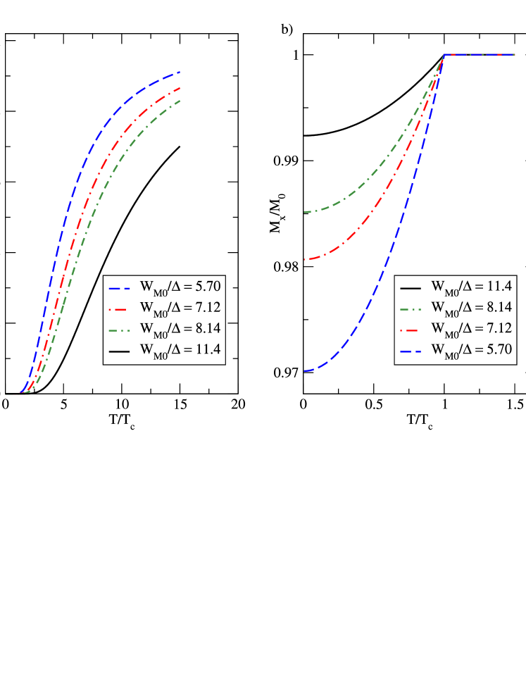
Figure 1: (Color online.) Temperature dependence of the magnetic moment induced by a weak magnetic field for different ratios of magnetic to superconducting order parameters.
a) $M_{z}(T)$: $M_{z}\rightarrow 0$ as $T\rightarrow 0$;
b) $M_{x}(T)$: $M_{x}$ stays finite as $T\rightarrow 0$.

In the zeroth order in $W_{Z}$ we neglect the R.H.S. of Eq. (44) and obtain the homogeneous equation

$$\bigl{[}\check{g}_{0}\,,\hat{\mathit{\Pi}}^{(z)}_{-}\bigr{]}=0\,.$$ (46)

In principle, any matrix function of $\hat{\mathit{\Pi}}_{-}^{(z)}$ satisfies Eq. (46). In order to find the function $\check{g}_{0}$ unambiguously one should check whether the solution satisfies the normalization imposed by Eq. (36) or not. This leads us to the solution

$$\check{g}_{0}=\frac{1}{\mathcal{E}_{S}}\hat{\mathit{\Pi}}_{-}^{(z)}\,,$$ (47)

where $\mathcal{E}_{S}^{2}=\omega_{n}^{2}+W_{M0}^{2}+|\Delta|^{2}$. It is easy to see that the solution given by Eq. (47) really satisfies the normalization condition

$$\check{g}_{0}\cdot\check{g}_{0}=\check{1}\,.$$ (48)

The correction $\delta\check{g}=\check{g}-\check{g}_{0}$ obeys the equation

$$\bigl{[}\delta\check{g}\,,\hat{\mathit{\Pi}}^{(z)}_{-}\bigr{]}=\mathcal{E}_{S}[\delta\check{g}\,,\check{g}_{0}]=-2\mathcal{E}_{S}\check{g}_{0}\cdot\delta\check{g}=iW_{Z}\bigl{[}\check{g}_{0}\,,\hat{\mathit{P}}\bigr{]}\,.$$ (49)

Here, we used the relation

$$\delta\check{g}\cdot\check{g}_{0}+\check{g}_{0}\cdot\delta\check{g}=0\,,$$ (50)

which follows from the normalization condition.

Using Eq. (48) we find from Eq. (49)

$$\delta\check{g}=-\frac{iW_{Z}}{2\mathcal{E}_{S}}\bigl{(}\check{g}_{0}\cdot\hat{\mathit{P}}\cdot\check{g}_{0}-\hat{\mathit{P}}\bigr{)}\,.$$ (51)

The matrix $\delta\check{g}$ can be written in an explicit form with the help of Eq. (47) and the expression for $\hat{\mathit{P}}$. We present here those parts of $\delta\check{g}$ that contribute to the magnetic moments, i.e. $\delta\check{g}_{x}$ and $\delta\check{g}_{z}$:

$$\delta\check{g}_{x}\equiv\delta\check{g}_{1} =-iW_{Z}\frac{|\Delta|^{2}}{\mathcal{E}_{S}^{3}}\hat{\rho}_{3}\cdot\hat{\tau}_{0}\cdot\hat{\sigma}_{1}\sin\theta\,,$$ (52)

$$\delta\check{g}_{z}\equiv\delta\check{g}_{3} =-iW_{Z}\frac{|\Delta|^{2}+W_{M0}^{2}}{\mathcal{E}_{S}^{3}}\hat{\rho}_{0}\cdot\hat{\tau}_{3}\cdot\hat{\sigma}_{3}\cos\theta\,.$$ (53)

Using Eqs. (39–40) we find for the spin polarization induced by the field $\mathbf{H}_{ex}$

$$M_{x} =M_{0}\left(1-2\pi T\sum_{\omega\geqslant 0}\frac{|\Delta|^{2}}{\mathcal{E}_{S}^{3}}\right)\sin\theta\,,$$ (54)

$$M_{z} =M_{0}\left(1-2\pi T\sum_{\omega\geqslant 0}\frac{|\Delta|^{2}+W_{M0}^{2}}{\mathcal{E}_{S}^{3}}\right)\cos\theta\,.$$ (55)

In principle, the sums over $\omega$ in Eqs. (54, 55) can be calculated at arbitrary temperatures but the final expressions are somewhat cumbersome. Therefore, we restrict ourselves by the limit of low temperatures $T~{}\rightarrow~{}0$. In this limit one replaces the sums over $\omega$ by integrals, which leads to the following expressions

$$M_{x} =M_{0}\frac{W_{M0}^{2}}{|\Delta|^{2}+W_{M0}^{2}}\sin\theta\,,$$ (56)

$$M_{z} =M_{0}\left(1-\int_{0}^{\infty}\frac{W_{M0}^{2}+|\Delta|^{2}}{\mathcal{E}_{S}^{3}}d\omega\right)\cos\theta\rightarrow 0\,.$$ (57)

Eq. (57) shows that in the limit of the perfect nesting ($\delta\mu~{}=~{}0$) the Knight shift vanishes at $T~{}=~{}0$ provided the applied magnetic field $\mathbf{H}$ is parallel to the orientation of the magnetization of the SDW. If the direction of $\mathbf{H}$ deviates from the $z$-direction, the Knight shift is finite and the induced magnetic moment $M_{x}$ approaches the spin magnetic moment of free electrons (Pauli paramagnetism) for $W_{M0}~{}\gg~{}\Delta$. The obtained results do not depend on the relation between $\Delta_{1}$ and $\Delta_{2}$ and thus are valid for both $s_{+-}$- and $s_{++}$- pairing.

In Fig.(1) we plot the temperature dependence of $M_{x}$ and $M_{z}$ for different ratios $W_{M0}/\Delta$ assuming that in the considered temperature range the magnetization $\mathbf{m}$ of the SDW depends only weakly on $T$.

At present, it is not easy to quantitatively compare our results obtained within a simplified model with available experimental data concerning the NMR studies in pnictides Chu ; Chu1 . There are several reasons for the difficulty and the major one is that the Knight shift is actually not discussed in those papers. Furthermore, the influence of the free electrons on the position of the NMR peak in the compound NaFeAs containing ²³Na atoms is weak because free electrons move in the FeAs planes. On the other hand, an internal local magnetic field of the SDW causes a stronger influence on the NMR peaks corresponding to the atoms ⁷⁵As. In addition, the ideal nesting is assumed in our model that leads to the fully gapped Fermi surface. This assumption is not fulfilled in materials studied in Refs. Chu ; Chu1 .

V Proximity Effect

We study the proximity effect considering a simple model: a contact between a superconductor with SDW (two order parameters: $\Delta$ and $W_{M}$), which we denote as $S_{SDW}$, and a conductor (or insulator at $W_{M}~{}\neq~{}0$ and low temperatures) with one order parameter (for example $W_{M}$) or with a simple normal metal $N$ ($\Delta~{}=~{}W_{M}~{}=~{}0$). Such a case may be realized in pnictides with a nonuniform doping level. We will find the quasiclassical retarded and advanced Green’s functions describing the equilibrium properties such as the density-of-states or the order parameters, $\Delta$ and $W_{M}$.

These Green’s functions obey the generalized Eilenberger equation. This equation is obtained from Eq. (29) by taking its element $(11)$ or $(22)$ and performing the Fourier transformation in the Matsubara representation.

As a result, we obtain

$$n_{x}v\partial_{x}\check{g}-\bigl{[}\check{g}\,,\hat{\mathit{\Pi}}_{\pm}^{(j)}\bigr{]}=0\,,$$ (58)

where $n_{x}=v_{x}/v=\cos\alpha$, $\alpha$ is the angle between the Fermi velocity $\mathbf{v}$ and the $x$-axis, and $v~{}=~{}|\mathbf{v}|$. The matrix $\hat{\mathit{\Pi}}_{\pm}^{(j)}$ is specified in Eq. (45).

We assume the $s_{+-}$-pairing and let the magnetization be directed along the $z$-axis. For simplicity, we assume as previously perfect nesting by putting $\delta\mu~{}=~{}0$.

Two different cases will be considered now:

• $\Delta^{\prime}(x)=\Delta_{0}$, $\Delta^{\prime\prime}(x)=0$, $W_{M0}(x)=W_{M0,S}$ for $x<0$ and $\Delta^{\prime}(x)=\Delta^{\prime\prime}(x)=0$, $W_{M0}(x)=W_{M0,M}$ for $x>0$

• $\Delta^{\prime}(x)=\Delta_{0}$, $\Delta^{\prime\prime}(x)=0$, $W_{M0}(x)=W_{M0,S}$ for $x<0$ and $\Delta^{\prime}(x)=\Delta^{\prime\prime}(x)=0$, $W_{M0}(x)=0$ for $x>0$

The second case corresponds to an interface between a superconductor with SDW and a normal (nonmagnetic) metal. We denote this type of contacts as $S_{SDW}/N$.

The first case corresponds to a system with SDW having the superconducting order parameter at $x<0$. This type of contact is denoted as $S_{SDW}/N_{SDW}$.

The contact between the two regions is assumed to be ideal and therefore all the functions should be continuous across the boundary $x~{}=~{}0$.

As in the previous section, we represent the solution $\check{g}(x)$ in the form

$$\check{g}(x)=\check{g}_{0}+\delta\check{g}(x)\,.$$ (59)

Here the matrix $\check{g}_{0}$ is a constant in space and obeys the equation

$$\bigl{[}\check{g}_{0}\,,\hat{\mathit{\Pi}}^{(z)}_{-}\bigr{]}=0\,.$$ (60)

The proper solution of this equation is written again in the form

$$\check{g}_{0}=\frac{1}{\mathcal{E}_{S}}\hat{\mathit{\Pi}}^{(z)}_{-}$$ (61)

with $\mathcal{E}_{S}^{2}=\omega_{n}^{2}+\Delta_{0}^{2}+W_{M0}^{2}$.

The matrix $\delta\check{g}(x)$ is not supposed to be small. It can be split into an even, $\check{s}$, and odd, $\check{a}$, in $n_{x}$ parts

$$\delta\check{g}=\check{s}+n_{x}\check{a}\,.$$ (62)

Substituting Eq. (62) into Eq. (58) and separating the even and odd in $n_{x}$ parts, we come to equations

$$v\partial_{x}\check{s}+\bigl{[}\hat{\mathit{\Pi}}^{(z)}_{-}\,,\check{a}\bigr{]} =0\,,$$ (63)

$$n_{x}^{2}v\partial_{x}\check{a}+\bigl{[}\hat{\mathit{\Pi}}^{(z)}_{-}\,,\check{s}\bigr{]} =0\,.$$ (64)

One can exclude the anisotropic part $\check{a}$ by differentiating Eq. (63) with respect to the coordinate $x$. Then, the equation for the isotropic part has the form

$$-l_{\alpha S}^{2}\frac{\partial^{2}\check{s}}{\partial x^{2}}+\frac{1}{2\mathcal{E}_{S}^{2}}\Bigl{(}\mathcal{E}_{S}^{2}\check{s}-\hat{\mathit{\Pi}}^{(z)}_{-}\check{s}\hat{\mathit{\Pi}}^{(z)}_{-}\Bigr{)}=0\,,$$ (65)

where $l_{\alpha S}=n_{x}v/2\mathcal{E}_{S}$ is a characteristic length of penetration of perturbations caused by the proximity effect into the superconductor with SDW. At low temperatures this length is determined by the smallest of the lengths $\{\xi_{\Delta}\simeq v/\Delta_{0},\xi_{M}\simeq v/W_{M0,M}\}$.

In the region $x>0$ the characteristic length is $l_{\alpha M}~{}=~{}n_{x}v/2\mathcal{E}_{M}$ (the case a)) or $l_{\alpha N}~{}=~{}n_{x}v/2\mathcal{E}_{\omega}$ (the case b)), where $\mathcal{E}_{M}^{2}~{}=~{}\omega_{n}^{2}~{}+~{}W_{M0,M}^{2}$ and $\mathcal{E}_{\omega}^{2}~{}=~{}\omega_{n}^{2}$.

We look for a solution of Eq. (65) in the form

$$\check{s}=\begin{cases}A(x)\hat{\tau}_{3}+B(x)\hat{\rho}_{3}\cdot\hat{\tau}_{2}\cdot\hat{\sigma}_{3}+C(x)\hat{\rho}_{1}\cdot\hat{\tau}_{2}\cdot\hat{\sigma}_{3}\,,&x<0\\ \tilde{A}(x)\hat{\tau}_{3}+\tilde{B}(x)\hat{\rho}_{3}\cdot\hat{\tau}_{2}\cdot\hat{\sigma}_{3}+\tilde{C}(x)\hat{\rho}_{1}\cdot\hat{\tau}_{2}\cdot\hat{\sigma}_{3}\,,&x>0\end{cases}$$ (66)

Substituting Eq. (66) into Eq. (65) one can rather easily find the functions $A$, $B$, $C$, etc.

$$A(x) =A_{0}\exp(x/l_{\alpha S})\,, \qquad\tilde{A}(x) =\tilde{A}_{0}\exp(-x/l_{\alpha M})\,,$$ (67)

$$B(x) =B_{0}\exp(x/l_{\alpha S})\,, \qquad\tilde{B}(x) =\tilde{B}_{0}\exp(-x/l_{\alpha M})\,,$$ (68)

$$C(x) =C_{0}\exp(x/l_{\alpha S})\,, \qquad\tilde{C}(x) =\tilde{C}_{0}\exp(-x/l_{\alpha M})\,,$$ (69)

$$A_{0}\omega_{n}+B_{0}\Delta_{0}+C_{0}W_{M0,S} =0\,,$$ (70)

$$\tilde{A}_{0}\omega_{n}+\tilde{C}_{0}W_{M0,S} =0\,.$$ (71)

We see that there are four independent arbitrary constants: $B_{0}$, $C_{0}$, $\tilde{B}_{0}$ and $\tilde{C}_{0}$ characterizing the solution $\check{s}$. They should be determined from the matching conditions that require the continuity of the matrices $\check{g}_{0}+\check{s}$ and $\check{a}$. The matching conditions are reduced to six equations four of which are independent and the other two follow from these four equations. Solving these equations, we find

$$A_{0} =\frac{\varsigma\varpi_{M}-\varpi_{S}}{1+\varsigma}\,, \qquad\tilde{A}_{0} =\frac{\varsigma\varpi_{S}-\varpi_{M}}{1+\varsigma}\,,$$ (72)

$$B_{0} =-\frac{1}{1+\varsigma}\Delta_{0}\,, \qquad\tilde{B}_{0} =\frac{\varsigma}{1+\varsigma}\Delta_{0}\,,$$ (73)

$$C_{0} =\frac{\varsigma\mathit{m}_{M}-\mathit{m}_{S}}{1+\varsigma}\,, \qquad\tilde{C}_{0} =\frac{\varsigma\mathit{m}_{S}-\mathit{m}_{M}}{1+\varsigma}\,.$$ (74)

where $\varsigma~{}=~{}(\varpi_{S}\varpi_{M}~{}+~{}\mathit{m}_{S}\mathit{m}_{M})^{-1}$, $\varpi_{S}~{}=~{}\omega/\mathcal{E}_{S}$, $\varpi_{M}~{}=~{}\omega/\mathcal{E}_{M}$ are the normalized Matsubara frequencies in the $SC$ and $M$ regions, and $\mathit{m}_{S,M}~{}=~{}W_{M0S,M}/\mathcal{E}_{S,M}$ are the magnetic order parameters in these regions. In the case of a contact of a superconductor with SDW and of a normal metal ($S_{SDW}/N$ contact), the energy $\mathcal{E}_{M}$ should be replaced by $\mathcal{E}_{\omega}$ and the quantity $W_{M0}$ set to be zero.

The amplitudes $\tilde{B}_{0}$, $\tilde{C}_{0}$ determine the penetration of the superconducting and magnetic correlations into the region with SDW or into the normal metal $N$ due to the proximity effect. The amplitudes $B_{0}$, $C_{0}$ describe the inverse proximity effect or, in other words, a suppression of $\Delta_{0}$ and $W_{M0}$ in the superconductor near the $S_{SDW}/N_{SDW}$ interface (or in the $S_{SDW}/N$ interface) due to the inverse proximity effect.

Note that, strictly speaking, in the case of the $S_{SDW}/N_{SDW}$ system we have to calculate the magnetic order parameter $M_{M0}$ self-consistently using the amplitude $\tilde{C}_{0}$. This makes the problem more difficult. However, the obtained results remain valid provided the quantity $W_{M0}$ is the same at $x>0$ and $x<0$ (i.e. $W_{M0,S}~{}=~{}W_{M0,M}~{}\equiv~{}W_{M0}$). In this case we obtain

$$A_{0} =-\frac{\omega\Delta_{0}^{2}}{\mathcal{E}_{S}\mathcal{E}_{M}(\mathcal{E}_{S}+\mathcal{E}_{M})}\,, \qquad\tilde{A}_{0} =0\,,$$ (75)

$$B_{0} =-\frac{\Delta_{0}\mathcal{E}_{M}}{\mathcal{E}_{S}(\mathcal{E}_{S}+\mathcal{E}_{M})}\,, \qquad\tilde{B}_{0} =\frac{\Delta_{0}}{\mathcal{E}_{S}+\mathcal{E}_{M}}\,,$$ (76)

$$C_{0} =\frac{m_{0}\Delta_{0}^{2}}{\mathcal{E}_{S}\mathcal{E}_{M}(\mathcal{E}_{S}+\mathcal{E}_{M})}\,, \qquad\tilde{C}_{0} =0\,.$$ (77)

The results obtained mean that the corrections to the DOS and to the magnetic order parameter determined by $\tilde{A}_{0}$ and $\tilde{C}_{0}$ are absent in this case. The superconducting pair function $\tilde{B}(x)$ penetrates the region with SDW over the length $l_{\alpha M}$ with the amplitude $\tilde{B}_{0}$. As it should be, this pair function penetrates the $N$ region over the length $l_{\alpha N}~{}=~{}l_{\alpha\omega}~{}=~{}|n_{x}|v/\omega_{n}$.

VI Josephson Effect

In this section, we calculate the dc Josephson current in an $S_{SDW}/N/S_{SDW}$ system using a simple model. We assume again an ideal nesting ($\delta\mu=0$) and take into account the impurity scattering in the self-consistent Born approximation. Then, the Eilenberger equation, Eq. (58), for the matrix $\check{g}$ acquires the form

$$n_{x}v\partial_{x}\check{g}-\bigl{[}\check{g}\,,\hat{\mathit{\Pi}}\bigr{]}=\frac{1}{2\tau}\bigl{[}\check{g}\,,\langle\check{g}\rangle\bigr{]}\,,$$ (78)

where the angle brackets stand for the average over the directions of the momentum and the matrix $\hat{\mathit{\Pi}}$ in the right (left) superconductors is equal to

$$\hat{\mathit{\Pi}}=\omega_{n}\hat{\tau}_{3}+\Delta\left(\hat{\rho}_{0,3}\cdot\hat{\tau}_{2}\cdot\hat{\sigma}_{3}\cos\left(\frac{\varphi}{2}\right)\pm\hat{\rho}_{3,0}\cdot\hat{\tau}_{1}\cdot\hat{\sigma}_{3}\sin\left(\frac{\varphi}{2}\right)\right)+W_{M0}\left(\hat{\rho}_{1}\cdot\hat{\tau}_{2}\cdot\hat{\sigma}_{3}\cos\left(\frac{\alpha}{2}\right)\mp\hat{\rho}_{2}\cdot\hat{\tau}_{1}\cdot\hat{\sigma}_{2}\sin\left(\frac{\alpha}{2}\right)\right)\,.$$ (79)

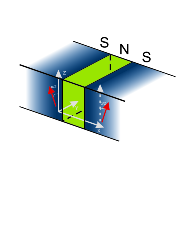
Figure 2: (Color online.) Josephson junction under consideration. A normal metal film is placed between two superconducting leads with SDW. The orientation of the magnetization vectors of the SDW in the leads lying in the $y$-$z$-plane is shown in red.

Eq. (79) corresponds to the case when the superconducting phase in the right (left) $S_{SDW}$ equals $\pm\varphi/2$ and the angle between the vector of the magnetization of the SDW and $z$-axis is equal to $\pm\alpha/2$ (cf. Fig. (2)). Considering the impurity scattering, we neglect interband scattering and regard, for simplicity, the impurity scattering time $\tau$ equal for each band. In the middle of the $N$ layer $\Delta~{}=~{}0$ and $W_{M0}~{}=~{}0$. We assume that the scattering time $\tau$ in this layer is rather short: $\hbar\tau^{-1}~{}\gg~{}T$ (diffusive limit).

As a boundary condition, we adopt the one obtained for a simplified model suggested in Ref. KL

$$\check{g}\left.\frac{\partial\check{g}}{\partial x}\right|_{x=\pm L}=\pm\gamma_{B}\bigl{[}\check{g}\,,\check{g}_{S}\bigr{]}\biggr{|}_{x=\pm L}\,,$$ (80)

where the parameter $\gamma_{B}~{}=~{}(2R_{B}\sigma_{N})^{-1}$ depends on the interface resistance $R_{B}$ per unit area and the conductivity $\sigma_{N}$ of the normal metal. This parameter is assumed to be a scalar, which means that we neglect transitions between different bands at the interfaces. In a more general case $\gamma_{B}$ is a matrix Millis ; EschrigBC ; NazarovBC .

We assume that the proximity effect is weak, which corresponds to small values of the parameter $\gamma_{B}\xi_{N}$, where $\xi_{N}~{}=~{}\sqrt{D/2\pi T}$. In this case the Green’s functions in the $S_{SDW}$ are only weakly perturbed by the contact with the $N$ layer (because of a large interface resistance) and the first term in Eq. (78) can be neglected. Then, the solution of Eq. (78) on the boundaries between the normal metal and superconductors can be written as

$$\check{g}_{S}(\pm L)=\check{g}_{+}\pm\check{g}_{-}\,,$$ (81)

where

$$\check{g}_{+}=\frac{1}{\mathcal{E}_{S}}\biggl{[}\omega_{n}\hat{\tau}_{3} +\Delta\hat{\rho}_{0,3}\cdot\hat{\tau}_{2}\cdot\hat{\sigma}_{3}\cos\left(\frac{\varphi}{2}\right)$$ (82)

$$+W_{M0}\hat{\rho}_{1}\cdot\hat{\tau}_{2}\cdot\hat{\sigma}_{3}\cos\left(\frac{\alpha}{2}\right)\biggr{]}$$

and

$$\check{g}_{-}=\frac{1}{\mathcal{E}_{S}}\biggl{[} \Delta\hat{\rho}_{3,0}\cdot\hat{\tau}_{1}\cdot\hat{\sigma}_{3}\sin\left(\frac{\varphi}{2}\right)$$ (83)

$$-W_{M0}\hat{\rho}_{2}\cdot\hat{\tau}_{1}\cdot\hat{\sigma}_{2}\sin\left(\frac{\alpha}{2}\right)\biggr{]}$$

with $\mathcal{E}_{S}^{2}=\omega_{n}^{2}+W_{M0}^{2}+\Delta^{2}$.

To find the Josephson current $\mathbf{j}_{J}$, we have to solve Eq. (78) in the $N$ layer, where $\Delta~{}=~{}0$ and $W_{M0}~{}=~{}0$. As usually, we represent the Green’s function $\check{g}$ as a sum of the symmetric and antisymmetric functions: $\check{g}~{}=~{}\check{s}~{}+~{}n_{x}\check{a}$ (see Eq. (62)). For $\check{s}$ and $\check{a}$ we obtain from Eq. (78) the following equations

$$v\partial_{x}\check{s}+\omega_{n}[\hat{\tau}_{3}\,,\check{a}] =-\frac{1}{2\tau}\left(\check{s}\check{a}-\check{a}\check{s}\right)\,,$$ (84)

$$v\langle n_{x}^{2}\partial_{x}\check{a}\rangle+\omega_{n}\bigl{[}\hat{\tau}_{3}\,,\langle\check{s}\rangle\bigr{]} =0\,,$$ (85)

where the angle brackets denote the angle averaging. In the diffusive limit considered here ($\tau T/\hbar~{}\ll~{}1$) the second term in Eq. (84) in the left hand side is small. The right-hand side can be transformed using the equation

$$\check{s}\check{a}+\check{a}\check{s}=0\,,$$ (86)

which follows immediately from the normalization condition Eq. (36). Then, we obtain for $\check{a}$

$$\check{a}=-l\check{s}\,\partial_{x}\check{s}\,.$$ (87)

We used another part of the normalization condition (for symmetric function)

$$\check{s}^{2}+n_{x}^{2}\check{a}^{2}=1\,,$$ (88)

in which the second term can be neglected (as follows from Eq. (88) $|\check{a}|~{}\ll~{}1)$. In the considered limit of a weak proximity effect ($|\check{s}|~{}\ll~{}1$) the matrix $\check{s}$ can be represented in the form

$$\check{s}=\hat{\tau}_{3}\,\mathrm{sgn}(\omega)+\delta\check{s}\,,$$ (89)

where the matrix $\delta\check{s}\approx\langle\delta\check{s}\rangle$ obeys the equation

$$-\frac{\partial^{2}\delta\check{s}}{\partial x^{2}}+\kappa_{\omega}^{2}\delta\check{s}=0$$ (90)

with $\kappa_{\omega}^{2}=2\omega_{n}/D$, $D=vl/3$ being the diffusion coefficient which is assumed to be the same in each band. Eq. (90) follows from Eq. (85) because, as we will see, the matrix $\delta\check{s}$ anticommutes with the matrix $\hat{\tau}_{3}$.

Eq. (90) has to be solved with the boundary conditions which follow from Eq. (80) and the representation Eq. (89)

$$\frac{\partial\delta\check{s}}{\partial x}(\pm L)=\pm\gamma_{B}\left[\check{g}_{S}(\pm L)-\hat{\tau}_{3}\frac{\omega}{\mathcal{E}_{S}}\right]\,.$$ (91)

The solution of Eq. (91) can easily be found in the form

$$\delta\check{s}(x)=\check{A}\cdot\frac{\cosh(\kappa_{\omega}x)}{\sinh(\kappa_{\omega}L)}+\check{B}\cdot\frac{\sinh(\kappa_{\omega}x)}{\cosh(\kappa_{\omega}L)}\,,$$ (92)

where

$$\check{A}=\frac{\gamma_{B}}{\mathcal{E}_{S}} \left[\Delta\hat{\rho}_{0,3}\cdot\hat{\tau}_{2}\cdot\hat{\sigma}_{3}\cos\left(\frac{\varphi}{2}\right)\right.$$ (93)

$$+ \left.W_{M0}\hat{\rho}_{1}\cdot\hat{\tau}_{2}\cdot\hat{\sigma}_{3}\cos\left(\frac{\alpha}{2})\right)\right]$$

and

$$\check{B}=\frac{\gamma_{B}}{\mathcal{E}_{S}} \left[\Delta\hat{\rho}_{3,0}\cdot\hat{\tau}_{1}\cdot\hat{\sigma}_{3}\sin\left(\frac{\varphi}{2}\right)\right.$$ (94)

$$- \left.W_{M0}\hat{\rho}_{2}\cdot\hat{\tau}_{2}\cdot\hat{\sigma}_{2}\sin\left(\frac{\alpha}{2}\right)\right]\,.$$

The Josephson current $j_{J}$ can be calculated using Eq. (37) and the expression for $\check{a}$ (87). We are interested in the part of $\check{a}$ which contributes to the current. This part can be written in the main approximation as

$$\check{a}=-l\,\delta\check{s}\,\partial_{x}\delta\check{s}\,.$$ (95)

Proceeding in this way we reduce the expression for the Josephson current $j_{J}$ to the form

$$j_{J}=\frac{i\sigma(2\pi T)}{8e}\sum_{\omega}\mathrm{Tr}\bigl{\{}\hat{\rho}_{3}\cdot\hat{\tau}_{3}\cdot\hat{\sigma}_{0}\cdot\delta\check{s}\,\partial_{x}\delta\check{s}\bigr{\}}\,.$$ (96)

Substituting Eqs. (92–94) into Eq. (96), we find

$$j_{J}=j_{c}\sin\varphi\,,$$ (97)

where the critical Josephson current $j_{c}$ is given by

$$j_{c}=\sigma\gamma_{B}^{2}L(2\pi T)\sum_{\omega}\frac{\Delta^{2}}{\mathcal{E}_{S}^{2}\theta_{\omega}\sinh(2\theta_{\omega})}\,,$$ (98)

where $\theta_{\omega}=\kappa_{\omega}L$. This formula differs from the expression for $j_{c}$ in an $S/N/S$ junction only by the term $W_{M0}^{2}$ in the energy $\mathcal{E}_{S}$. The presence of this term leads to a suppression of the current $j_{c}$ provided $W_{M0}$ is not small compared to the superconducting energy gap $\Delta$. Note that, in our simple model, the Josephson critical current does not depend on the mutual orientation of the vectors of the magnetization in the left and right superconductors $S_{SDW}$.

It is of interest to calculate the spin current in the Josephson junction. The spin current is given by Eq. (41). Using Eq. (87) one can write the spin current between the superconductors as

$$j_{sp,x}^{(x)}=-\frac{(2\pi T)D\nu\mu_{B}}{8e}\sum_{\omega}\mathrm{Tr}\bigl{\{}\hat{\rho}_{3}\cdot\hat{\tau}_{3}\cdot\hat{\sigma}_{1}\cdot\delta\check{s}\,\partial_{x}\delta\check{s}\bigr{\}}\,,$$ (99)

where the upper index means the spin orientation, and the lower stands for the direction of the current. Substituting Eqs. (92–94), we obtain from Eq. (99)

$$j_{sp,x}^{(x)}=\gamma_{B}^{2}L(2\pi T)D\nu\mu_{B}\sum_{\omega}\frac{W_{M0}^{2}}{\mathcal{E}_{S}^{2}\theta_{\omega}\sinh(2\theta_{\omega})}\sin\alpha\,.$$ (100)

Eq. (100) resembles the Josephson expression for the supercurrent. Both formulas contain sine of an angle. In the conventional Josephson formula this angle is equal to the difference of the phases of the superconductors, whereas the angle $\alpha$ in the expression for the spin current in Eq. (100) determines the mutual orientation of the SDW in the right and left electrodes. Eq. (99) is valid also above the superconducting transition temperature $T_{c}$, when $\Delta~{}=~{}0$. This current is dissipationless like the Josephson current. The nature of a similar dissipationless spin current in systems which differ from ours has been discussed in Ref. MacDonald

VII Discussion

We have derived equations for the quasiclassical Green’s functions for a two-band superconductor with an SDW. It was assumed that the Fermi velocities in the electron and hole bands are equal. We neglected the anisotropy of the Fermi surfaces.

Using these equations and assuming the ideal nesting, we considered three problems: the Knight shift, the proximity effect and the dc Josephson effect. It was shown that, provided the direction of the applied magnetic field coincides with the direction of the magnetization $\mathbf{m}$ in the SDW, the Knight shift vanishes at zero temperature and in the absence of the spin-orbit interaction. If the magnetic field is not collinear with the $\mathbf{m}$ vector, the Knight shift is finite, which correlates with the results of a recent paper, Ghaemi where it was shown that the DOS of a superconductor with the SDW also depends on the orientation of the external magnetic field.

We have demonstrated that near the interface between the superconductor with the SDW and a normal metal the components of $\check{g}$ describing both magnetic and superconducting correlations penetrate into the normal metal over the length of the order $\min\{\hbar v/W_{M0},\hbar v/\Delta\}$.

Using the simplest model of the $S_{SDW}/N/S_{SDW}$ Josephson junction, we calculated the critical Josephson current and showed that, in this model, it does not depend on the mutual orientation of the magnetization in the superconductors with the SDW.

However, the dissipationless spin current ($j_{sp}$), which arises in the junction, depends on the misorientation angle between the magnetisations of the SDW, $\alpha$, in the same way ($j_{sp}\sim\sin\alpha$) as the Josephson current $j_{J}$ depends on the phase difference of the superconducting order parameter.

Although the equations for the quasiclassical Green’s functions have been derived using the simplest model of a two-band superconductor with an SDW, we believe that the results obtained on the basis of this model remain valid, at least qualitatively, for more complicated models describing realistic materials.

The derived equations can be easily generalized to the case of impurity scattering and can be applied to different problems, equilibrium and nonequilibrium (ac Josephson effects in $S_{SDW}/N/S_{SDW}$ junctions, vortices, etc.).

Note added in proof. Although Eqs. (29, 36) for the quasiclassical Green’s functions for two-band superconductors with the SDW are valid for arbitrary deviation from the ideal nesting ($\mu~{}\neq~{}0$), we assumed the ideal nesting ($\mu~{}=~{}0$) when applying these equations to the study of particular effects. This assumption is justified, strictly speaking, in a hypothetical case of equal critical transition temperatures ($T_{cS}~{}=~{}T_{cSDW}$) or in the case of a metastable states (when a first-order transition takes place). In real materials $\mu~{}\neq~{}0$, and therefore one has to take into account the dependence of the order parameters ($\Delta$ and $W_{M}$) and other quantities on $\mu$. For example, one can show that the Josephson critical current $j_{c}$ contains an additional term $\delta j_{c}$ which is negative and depends on the angle $\alpha$: $\delta j_{c}~{}\sim~{}-\mu^{2}\cos^{2}\alpha$.

VIII Acknowledgements

The authors are grateful to I. Eremin for useful remarks and discussions. We thank SFB 491 for financial support.

References

- (1) A. Buzdin, Rev. Mod. Phys. 77, 935 (2005).
- (2) F. S. Bergeret, A. F. Volkov, K. B. Efetov, Rev. Mod. Phys. 77, 1321 (2005).
- (3) M. Eschrig, Physics Today, 64(1), 43 (2011).
- (4) R. S. Keizer, S. T. B. Goennenwein, T. M. Klapwijk, G. Miao, G. Xiao, A. Gupta, Nature 439, 825 (2006).
- (5) I. Sosnin, H. Cho, V. T. Petrashov, and A. F. Volkov, Phys. Rev. Lett. 96, 157002 (2006).
- (6) T. S. Khaire, M. A. Khasawneh, W. P. Pratt, Jr., N. O. Birge, Phys. Rev. Lett. 104, 137002 (2010).
- (7) J. W. A. Robinson, J.D.S. Witt, M. G. Blamire, Science 329, 59 (2010).
- (8) D. Sprungmann, K. Westerholt, H. Zabel, M. Weides, H. Kohlstedt, Phys. Rev. B 82, 060505 (2010).
- (9) M. S. Anwar, M. Hesselberth, M. Porcu, J. Aarts, Phys. Rev. B 82, 100501 (2010).
- (10) L. Bulaevskii, A. Buzdin, M. Kulic, and S. Panjukov, Adv. Phys. 34, 175 (1985).
- (11) N. Kulikov and V. V. Tugushev, Sov. Phys. Usp. 27, 954 (1984).
- (12) A. A. Gorbatsevich, V. Ph. Elesin, and Yu. V. Kopaev, Phys. Lett. A 125, 149 (1987).
- (13) A. Aperis, G. Varelogiannis, P. B. Littlewood, and B. D. Simmons, J. Phys.: Condens. Matter 20, 434235 (2008).
- (14) R. L. Greene and P. M. Chaikin, Physica 126B, 431 (1984).
- (15) Y. Kamuhara et al., J. Am. Chem. Soc. 130, 3296 (2008).
- (16) X. H. Chen et al., Nature 453, 761 (2008).
- (17) G. F. Chen et al., Phys. Rev.Lett. 100, 247002 (2008).
- (18) M. Rotter, M. Tegel, and D. Johrendt, 101, 107006 (2008).
- (19) C. Wang et al., Europhys. Lett, 83, 67006 (2008).
- (20) J. A. Wilson, J. Phys.: Condens. Matter 22, 203201 (2010).
- (21) D. C. Johnston, Adv. Phys. 59, 803 (2010).
- (22) Z. P. Yin, K. Haule, G. Kotliar, Nature Phys. 7, 294 (2011).
- (23) E. G. Moon and S. Sachdev, Phys. Rev. B 82, 104516 (2010).
- (24) I. I. Mazin, D. J. Singh, D. M. Johannes, and M. H. Du, Phys. Rev.Lett. 101, 057003 (2008).
- (25) A. B. Vorontsov, M. G. Vavilov, and A. V. Chubukov, Phys. Rev. B 79, 060508(R) (2009).
- (26) A. B. Vorontsov, M. G. Vavilov, and A. V. Chubukov, Phys. Rev. B 81, 174538 (2010).
- (27) R. M. Fernandes and J. Schmalian, Phys. Rev. B 82, 014521 (2010).
- (28) V. Cvetkovic and Z. Tesanovic, Phys. Rev. B 80, 024512 (2009).
- (29) N. Lee and Han-Y. Choi, Phys. Rew. B 82, 174508 (2010).
- (30) A. F. Kemper, T. A. Maier, S. Graser, H.-P. Cheng, P. J. Hirschfeld, and D. Scalapino, New J. Phys. 12, 073030 (2010).
- (31) J.-P. Ismer, I. Eremin, E. Rossi, D. K. Morr, and G. Blumberg, Phys. Rev. Lett. 105, 037003 (2010).
- (32) X. H. Zhang et al., Phys. Rev.Lett. 102, 147002 (2009).
- (33) Y. R. Zhou et al., arXiv:arXiv:0812.3295 (2009) [cond-mat].
- (34) T. Katase et al., Appl. Phys. Lett., 96, 142507 (2010).
- (35) S. Schmidt et al., Appl. Phys. Lett. 97, 172504 (2010).
- (36) D. Parker and I. I. Mazin, Phys. Rev. Lett. 102, 227007 (2009).
- (37) W.-Q. Chen and F.-C. Zhang, arXiv:1009.4756 [cond-mat].
- (38) I. B. Sperstad, J. Linder, and A. Sudbø, Phys. Rev. B 80, 144507 (2009).
- (39) G. Eilenberger, Z. Phys. 214, 195 (1968).
- (40) K. Usadel, Phys. Rev. Lett. 25, 507 (1970).
- (41) A. I. Larkin and Yu. N. Ovchinnikov, in Nonequilibrium Superconductivity, edited by D.N. Langenberg and A.I. Larkin (Elsevier, Amsterdam, 1984).
- (42) S. N. Artemenko and A. F. Volkov, in Charge Density Waves in Solids, edited by L. P. Gor’kov and G. Grüner, (Elsevier, Amsterdam, 1989).
- (43) L. P. Gor’kov, G. B. Teitel’baum, Phys. Rev. B 82, 020510 (2010).
- (44) A. E. Koshelev and A. A. Golubov, Phys. Rev. Lett. 90, 177002 (2003).
- (45) V. Vorontosv and I. Vekhter, Phys. Rev. B 75, 224501 (2007); arXive: 1006.0738 [cond-mat].
- (46) A. Anishchanka, A. F. Volkov, and K. B. Efetov, Phys. Rev. B 76, 104504 (2007).
- (47) A. Gurevich, Phys. Rev. B 82, 184504 (2010).
- (48) J. Rammer and H. Smith, Rev. Mod. Phys. 58, 323 (1986).
- (49) W. Belzig, G. Schoen, C. Bruder, and A.D. Zaikin, Superlattices and Microstructures, 25, 1251 (1999).
- (50) N. B. Kopnin, Theory of Nonequilibrium Superconductivity (Clarendon Press, Oxford, UK, 2001).
- (51) G. M. Androes and V. D. Knight, Phys. Rev. 121, 779 (1961).
- (52) A. A. Abrikosov and L. P. Gor’kov, Sov. Phys. JETP, 15, 752 (1962).
- (53) M. Klanjesek et al., arXiv: 1011.1387 [cond-mat].
- (54) P. Jeglic et al., Phys. Rev. B 79, 094515 (2009); ibid 81, 140511 (2010).
- (55) M. Yu. Kupriyanov and V. F. Lukichev, JETP 67, 1163 (1988).
- (56) A. Millis, D. Rainer, and J. A. Sauls, Phys. Rev. B 38, 4504 (1988).
- (57) M. Eschrig, Phys. Rev. B 80, 134511 (2009).
- (58) A. Cottet, D. Huertas-Hernando, W. Belzig, Yu. V. Nazarov, Phys. Rev. B 80, 184511 (2009).
- (59) J. König, M. C. Bönsager, and A. H. MacDonald, Phys. Rev. Lett. 87, 187202 (2001); J. Heurich, J. König, and A. H. MacDonald, Phys. Rev. B 68, 064406 (2003).
- (60) Pouyan Ghaemi and Ashvin Viswanath, arXive: 1002.4638 [cond-mat].