Josephson Currents in Quantum Hall Devices

Abstract

We consider a simple model for an SNS Josephson junction in which the “normal metal” is a section of a filling-factor $\nu=2$ integer quantum-Hall edge. We provide analytic expressions for the current/phase relations to all orders in the coupling between the superconductor and the quantum Hall edge modes, and for all temperatures. Our conclusions are consistent with the earlier perturbative study by Ma and Zyuzin [Europhysics Letters 21 941-945 (1993)]: The Josephson current is independent of the distance between the superconducting leads, and the upper bound on the maximum Josephson current is inversely proportional to the perimeter of the Hall device.

I Introduction

The zero-voltage Josephson current in a supercondictor/normal-metal/superconductor (SNS) junction [1] arises from Andreev scattering [2] at the SN and NS interfaces. In the ideal case, an electron incident on one superconductor from the normal metal will be reflected back into the normal metal as a hole, and this hole, on striking the second superconductor, will be reflected back towards the first superconductor as an electron. When the relative phase of the order parameters is such that constructive interference occurs, the back-and-forth process continues ad infinitum and transfers two electrons from superconductor to superconductor in each cycle [4, 5, 6, 7, 3]. A round trip takes time $2W/v_{F}$, where $v_{F}$ is the Fermi velocity and $W$ the separation between the superconductors. The current will therefore be $ev_{F}/W$ for each open transverse channel. In practice, the probability of Andreev reflection is less than unity [8, 9] and the motion in the metal may be diffusive, but $ev_{F}/W$ per channel remains an upper bound on the critical current.

An interesting question arises as to what happens when the “normal” metal consists of the chiral fermions at the edge of a quantum Hall (QH) bar [10]. In this case the holes move in the same direction as the electrons, so conventional Andreev retro-reflection is impossible. A two-electron charge transfer requires a (phase coherent) passage around the entire perimeter of the Hall bar, and this lengthy excursion suggests that the small “$W$” of the conventional junction be replaced by the much larger perimeter $L$ of the Hall bar. A perturbative study of a S-QH-S system in [11] supports this conclusion and estimates that the maximum Josephson current will be very small — in the order of 1 nA for mm scale devices. In view of ongoing experiments on quantum-Hall Josephson junctions, however, it seems worth revisiting the problem to see if devices might be engineered to provide larger critical currents.

In this paper we introduce a model of an S-QH-S junction that is simple enough that it can be studied non-perturbatively. We obtain analytic expressions for the Josephson current/phase relation to all orders in the S-QH coupling, and at all temperatures. Despite our greater control over the model, the key conclusions of the perturbative studies in [11] (see also [12]) are unchanged: at filling fraction $\nu=2$ an upper bound for the critical Josephson current is given by $2ev_{d}/L$ where $v_{d}$ is the edge-mode drift velocity and $L$ is the perimeter of the Hall device. Further, the temperature scale at which the Jospehson current is washed out by thermal effects is set by the edge-mode level spacing $E_{n+1}-E_{n}=2\pi\hbar v_{d}/L$. Thus, if we wish to see Josephson-junction physics in quantum Hall devices, we should construct the junctions by coupling superconducting probes to meso-scale Hall-dots.

In section two we introduce the model and solve the associated Bogoliubov-de Gennes equation. In section three we introduce an analytic regularization scheme to handle the otherwise ill defined sums that appear in the current/phase relation. In section four we demonstrate that our regularization scheme is consistent with conventional perturbation theory at both zero and non-zero temperature. We finish with a brief discussion of effects that we have not taken into account, and that may or may not be significant.

II The model

We consider a $\nu=2$ quantum-Hall edge (two spins therefore) in interaction with superconducting (SC) leads (figure 1). We model the system by a linear-dispersion edge-mode hamiltonian

$$H=\oint\left\{-iv_{d}\psi^{\dagger}_{\uparrow}(\partial_{x}-ieA)\psi_{\uparrow}-iv_{d}\psi^{\dagger}_{\downarrow}(\partial_{x}-ieA)\psi_{\downarrow}\right.\quad$$

$$\left.+|\Delta(x)|e^{i\theta(x)}\psi^{\dagger}_{\uparrow}\psi^{\dagger}_{\downarrow}+|\Delta(x)|e^{-i\theta(x)}\psi_{\downarrow}\psi_{\uparrow}\right\}dx.$$ (1)

Here $v_{d}$ is the edge-mode drift velocity that is proportional to the gradient of the confining potential. The terms with $\Delta(x)$ are non-zero only where the edge state lies under the superconducting leads. They account for the Andreev coupling arising from the two-dimensional electron gas (2DEG) wavefunctions reaching up to touch the superconductor as they drift under the electrodes. (See figure 2.) In contrast to the usual proximity effect, the topological protection of the QH edge modes means that this interaction cannot open a gap — but it may, for example, convert a charge-$(e)$ right-going spin-up electron into a charge-$(-e)$ right-going spin-up hole, and in the process transfer a spin-singlet pair of charge-$(e)$ electrons from the Hall bar to the superconductor where they merge with the S-wave condensate.

We have not included Zeeman-energy term to spilt the energy between the spin up and spin down edge modes. Such a term adds only a multiple of the identity matrix to the BdG operator, and so has no effect on the subsequent analysis. Further, we assume that the energy scales of relevance are smaller than the energy gap of of the superconducting leads. We therefore regard the parameters $|\Delta|$ as being externally imposed, and not to depend the energy of the Hall-bar electrons, or on the temperature.

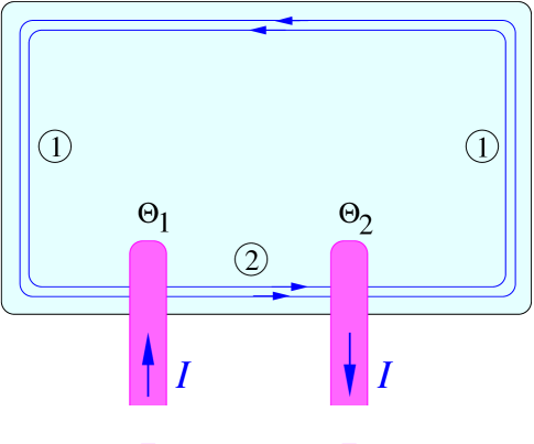
Figure 1: A Hall bar with superconducting probes passing a current $I$ through the edge modes. The circled numbers label the regions (1) “outside the leads,” and (2) “between the leads.”

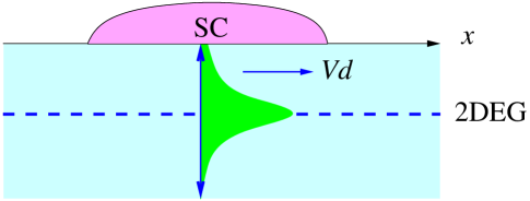
Figure 2: The wavefunction for an electron in a 2DEG is confined in the vertical direction, but there is some amplitude for the vertically oscillating electron to touch the superconductor. As a slowly-drifting Landau-level wavepacket passes under the superconducting lead, there will be many opportunities for Andreev reflection to turn the electron into a hole.

We can rewrite $H$ in the BdG form

$$H=\int dx\left\{\left(\matrix{\psi^{\dagger}_{\uparrow},\psi_{\downarrow}}\right)\left[\matrix{-iv_{d}(\partial_{x}-ieA)&|\Delta(x)|e^{i\theta(x)}\cr|\Delta(x)|e^{-i\theta(x)}&-iv_{d}(\partial_{x}+ieA)}\right]\left(\matrix{\psi_{\uparrow}\cr\psi^{\dagger}_{\downarrow}}\right)\right\}+const.$$ (2)

Here we have used an integration by parts together with the anticommutation property of the Fermi fields to write

$$\int\{\psi^{\dagger}_{\downarrow}(-iv_{d}(\partial_{x}-ieA))\psi_{\downarrow}\}dx=\int\{\psi_{\downarrow}(-iv_{d}(\partial_{x}+ieA))\psi^{\dagger}_{\downarrow}\}dx+const.$$ (3)

This rewriting is essentially a charge-conjugation transformation that makes manifest the particle-hole symmetry of the linearized edge spectrum. In particular, it reveals that the charge-$(-e)$ spin-up holes created by $\psi_{\downarrow}$ move in the same direction as the charge-$(e)$ spin-up electrons created by $\psi^{\dagger}_{\uparrow}$. The “constant” contains the truly constant ground-state energy of the spin down electrons, but also the term $-v_{d}e\int\delta(0)A(x)\,dx$ that subtracts a background electric charge. This charge gets discarded as we switch to the charge-conjugate picture in which charge-$(-e)$ holes occupy the states that are not occupied by electrons. Keeping track of the “constant” restores the physical charge when needed.

The vector potential $A$ acts as a chemical potential and controls the location of the Fermi energy. In much of our discussion we will assume that when $\Delta=0$ the Fermi energy lies midway between two edge-mode energy levels. This assumption is for illustrative purposes only. Indeed the detailed current/phase relation will depend sensitively on the exact location of the Fermi energy relative to the edge modes because varying $\theta$ can make a level cross the Fermi energy, change its occupation, and cause a jump in the Josephson current. The sensitivity will manifest itself as Bohm-Aharonov oscillations in the Josephson current as a function of the magnetic flux through the Hall bar [11].

For our mid-spaced $E_{F}$ we can make a gauge transformation to set $A\to 0$ at the expense of changing periodic boundary conditions to antiperiodic ones, and simultaneously redefining $\theta(x)$. We assume that we have done this. The Bogoliubov-deGennes (BdG) equation for the eigenmodes is therefore

$$\left[-iv_{d}{\partial\over\partial x}+|\Delta(x)|e^{i\sigma_{3}\theta(x)}\sigma_{1}\right]\left(\matrix{u\cr v}\right)=E\left(\matrix{u\cr v}\right).$$ (4)

Equation (4) has a path-ordered exponential solution

$$\left(\matrix{u(x)\cr v(x)}\right)=e^{iEx/v_{d}}\,{\rm P}\exp\left\{-i\int_{0}^{x}K(\xi)\,d\xi\right\}\left(\matrix{u(0)\cr v(0)}\right),$$ (5)

where $K(x)=|\Delta(x)|e^{i\sigma_{3}\theta(x)}\sigma_{1}/v_{d}$ is a hermitian matrix. Note that, in distinction to the usual BdG case, we did not double the number of degrees of freedom when we constructed the BdG operator, so all the BdG eigenmodes are needed.

Only a part $\Omega$ (the union of the two regions under the SC electrodes) of the perimeter of the Hall bar is in contact with the superconductor, and we set

$$U={\rm P}\exp\left\{-i\int_{\Omega}K(\xi)\,d\xi\right\}\in{\rm SU}(2).$$ (6)

As the perimeter of the Hall bar forms a closed loop, it was reasonable to impose periodic boundary conditions, but recall that these were changed to antiperiodic boundary conditions by the gauge transformation that removed $A(x)$. The eigenmodes of the BdG operator Hamiltonian are therefore determined from the eigenvalues of $U$ by requiring that

$$\left(\matrix{u_{n}\cr v_{n}}\right)=-e^{iE_{n}L/v_{d}}U\left(\matrix{u_{n}\cr v_{n}}\right).$$ (7)

Here $L$ is the length of the Hall-bar perimeter. Now the eigenvalues of $U$ will be of the form $e^{\pm i\phi}$ and so the energy eigenvalues are given by the requirement that $(E_{n}L/v_{d})\pm\phi=\pi(2n+1)$, or

$$E_{n}={v_{d}\over L}\left(\pi(2n+1)\mp\phi\right).$$ (8)

Note that if $(u,v)^{T}$ is an eigenvector of $U$ with eigenvalue $e^{i\phi}$ then $-i\sigma_{2}(u^{*},v^{*})=(-v^{*},u^{*})$ is an eigenvector of $U$ with eigenvalue $e^{-i\phi}$. Consequently if $(u_{n}(x),v_{n}(x))^{T}$ is an eigenfunction of the BdG operator corresponding to eigenvalue $E_{n}$, then $(-v^{*}_{n}(x),u^{*}_{n}(x))^{T}$ is an eigenfunction corresponding to energy $-E_{n}$. These facts follow from

$$(i\sigma_{2})\sigma_{i}(-i\sigma_{2})=-\sigma_{i}^{*}\quad\Longrightarrow\quad(i\sigma_{2})U^{*}(-i\sigma_{2})=U,$$ (9)

and give rise to the usual antilinear S-wave BdG particle-hole symmetry “$C$” with $C^{2}=-{\rm Id}$. This symmetry must be distinguished from the approximate particle-hole symmetry arising from our linearization of the quantum Hall edge-mode spectrum.

If the phase of the order parameter is constant in segments $\Omega_{1,2}$ (the superconducting leads) then $U=U_{2}U_{1}$ where

$$U_{a}=\left[\matrix{\cos D_{a}&-ie^{i\theta_{a}}\sin D_{a}\cr-ie^{-i\theta_{a}}\sin D_{a}&\cos D_{a}}\right],\quad a=1,2.$$ (10)

Here $D_{a}=|\Delta|w_{a}/v_{d}$ where $w_{a}$ is the width of lead $a$. The eigenvalues of $U$ are $e^{\pm i\phi}$, and, by taking the trace of $U$, we see that $\phi$ is given by the spherical cosine rule:

$$\cos\phi=\cos D_{1}\cos D_{2}-\cos\theta\sin D_{1}\sin D_{2}.$$ (11)

The spherical triangle (see figure 3) arises because the matrices $U_{1}$ and $U_{2}$ are the spinor representations of successive ${\rm SO}(3)$ rotations through angles $2D_{1}$ and $2D_{2}$ about axes separated by the angle $\theta$. It is shown in [13] that such rotations can be combined through the use of mirrors that form the geodesic sides of the triangle.

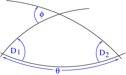
Figure 3: The spherical triangle that relates the eigen-phase $\phi$ to the order-parameter phase difference $\theta=\theta_{2}-\theta_{1}$.

From now on we understand by “$\phi$”, the solution of (11) that lies in the range $0\leq\phi\leq\pi$, and by the vector $(u,v)^{T}$ the corresponding eigenvector of $U$. We similarly take “$E_{n}$” to mean the combination

$$E_{n}={v_{d}\over L}\left(2\pi(n+1/2)-\phi\right).$$ (12)

Now we make the Bogoliubov transformation

$$\left(\matrix{\psi_{\uparrow}(x)\cr\psi^{\dagger}_{\downarrow}(x)}\right)=\sum_{n=-\infty}^{\infty}\left\{b_{n\uparrow}\left(\matrix{u_{n}(x)\cr v_{n}(x)}\right)+b^{\dagger}_{n\downarrow}\left(\matrix{-v_{n}^{*}(x)\cr\phantom{-}u_{n}^{*}(x)}\right)\right\}.$$ (13)

In order not to over-count, we ensure that the modes are those that, after passing the superconductor, take the form $(u_{n}(x),v_{n}(x))=e^{i(E_{n}x+\phi)}(u,v)$, and $(-v^{*}_{n}(x),u^{*}_{n}(x))=e^{-i(E_{n}x/v_{d}+\phi)}(-v^{*},u^{*})$. The Fermionic anticommutation relations coupled with the BdG eigenfunction completeness relations then require that

$$\{b_{n\downarrow},b_{m\downarrow}\}=\{b_{n\uparrow},b_{m\uparrow}\}=\{b_{n\downarrow},b_{m\uparrow}\}=\{b^{\dagger}_{n\downarrow},b^{\dagger}_{m\uparrow}\}=0,$$ (14)

and

$$\{b^{\dagger}_{n\downarrow},b_{m\downarrow}\}=\{b^{\dagger}_{n\uparrow},b_{m\uparrow}\}=\delta_{nm}.$$ (15)

The Bogoliubov transformation simplifies $H$ to

$$H=\sum_{n=-\infty}^{\infty}E_{n}(b^{\dagger}_{n\uparrow}b_{n\uparrow}-b_{n\downarrow}b^{\dagger}_{n\downarrow})+const,$$ (16)

the “constant” being the same one that was introduced earlier. It is not really a constant as it depends on the gauge field $A$, but it is independent of $\theta(x)$. Recall that the $A$ dependence accounts for the total charge of the spin-down Fermi sea that was discarded when we made the particle-hole interchange for this spin component. The minimum-energy state is defined by the properties

$$b_{n\uparrow}{|0\rangle}=0, E_{n}>0,$$

$$b^{\dagger}_{n\uparrow}{|0\rangle}=0, E_{n}<0,$$

$$b_{n\downarrow}{|0\rangle}=0, E_{n}>0,$$

$$b^{\dagger}_{n\downarrow}{|0\rangle}=0, E_{n}<0.$$ (17)

Using these, we compute the ground state energy to be

$$E_{\rm ground}=\sum_{E_{n}<0}E_{n}-\sum_{E_{n}>0}E_{n}.$$ (18)

The quantity $E_{\rm ground}$ is formally divergent, but the physics resides entirely in the variation of $E_{\rm ground}$ with the phase difference $\theta=\theta_{2}-\theta_{1}$. Now as we vary $\theta$ all $E_{n}$ move in the same direction. The energy dependence on $\theta$ largely cancels between the two sums. In order to extract the small, but non-zero, residuum we will have to regulate the sums in a controlled manner. This we do in the next section.

III Computing the current

Given a Dirac-like spectrum of energy levels $-\infty<E_{n}<\infty$, the associated ground-state charge and current can often be expressed in terms of the spectral asymmetry [14]. This quantity is defined [15, 16] to be the regulated sum

$$\eta=\lim_{s\to 0}\left\{-\sum_{n=-\infty}^{\infty}{\rm sgn}(E_{n})e^{-s|E_{n}|}\right\}.$$ (19)

For energies of our form, $E_{n}=\alpha(2\pi(n+1/2)-\phi)$, a direct calculation shows that for $-\pi<\phi<\pi$, we have

$$\left\{-\sum_{n=-\infty}^{\infty}{\rm sgn}(E_{n})e^{-s|E_{n}|}\right\}=-{\phi\over\pi}-{1\over 6\pi}\left(\phi^{3}-\phi\pi^{2}\right)(\alpha s)^{2}+O(s^{4}).$$ (20)

Thus

$$\eta(\phi)=-{\phi\over\pi},\quad-\pi<\phi<\pi,$$ (21)

and extends with $2\pi$ periodicity in $\phi$, (see figure 4).

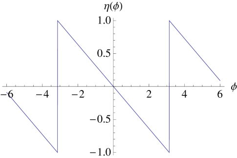
Figure 4: A plot of $\eta(\phi)$ showing the $2\pi$ periodicity.

We may similarly define and compute an analytically-regulated version of the ground-state energy (18):

$$(E_{\rm ground})_{\rm reg}=\lim_{s\to 0}\left\{-\sum_{n=-\infty}^{\infty}{\rm sgn}(E_{n})E_{n}e^{-s|E_{n}|}+{1\over\pi\alpha s^{2}}\right\}=\alpha\left({\phi^{2}\over 2\pi}-{\pi\over 6}\right),\quad-\pi<\phi<\pi.$$

This quantity also extends periodically outside the range $-\pi<\phi<\pi$ — see figure 5. The subtraction needed for the existence of the limit is independent of $\phi$, and the constant $-\alpha\pi/6$ is the same as would be obtained by zeta-function regularization [17]. Let us also compute

$$\left({dE_{\rm ground}\over d\phi}\right)_{\rm reg} \stackrel{{\scriptstyle\rm def}}{{=}} \lim_{s\to 0}\left\{-\sum_{n=-\infty}^{\infty}{\rm sgn}(E_{n})\left({dE_{n}\over d\phi}\right)e^{-s|E_{n}|}\right\}$$

$$= \lim_{s\to 0}\left\{\alpha\sum_{n=-\infty}^{\infty}{\rm sgn}(E_{n})e^{-s|E_{n}|}\right\}$$

$$= \alpha{\phi\over\pi},$$

and observe that the regulated energy possesses the comforting property that

$${d\over d\phi}(E_{\rm ground})_{\rm reg}=\left({dE_{\rm ground}\over d\phi}\right)_{\rm reg}.$$ (22)

We will relate these energy derivatives to the ground-state expectation value of the divergence of the current operator.

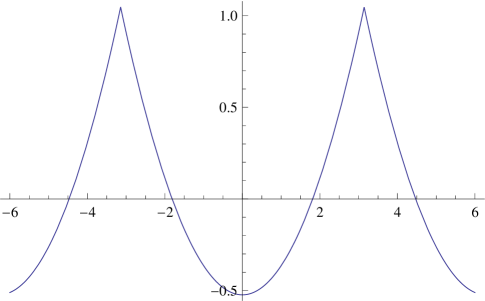
Figure 5: A plot of $\alpha^{-1}(E_{\rm ground}(\phi))_{\rm reg}$ showing the $2\pi$ periodicity

The current operator is

$$j(x){=}-{\delta H\over\delta A(x)}.$$ (23)

If we include the contribution from the $A$ dependent “constant” when taking the functional derivative, then the ground state current is

$${\langle j(x)\rangle} = ev_{d}{\langle 0|\psi^{\dagger}_{\uparrow}(x)\psi_{\uparrow}(x)+\psi^{\dagger}_{\downarrow}(x)\psi_{\downarrow}(x)|0\rangle}$$ (24)

$$= 2ev_{d}\left(\sum_{E_{n}<0}|u_{n}(x)|^{2}+\sum_{E_{n}>0}|v_{n}(x)|^{2}\right).$$

If we ignore the “constant,” the current becomes

$${\langle j(x)\rangle} = ev_{d}{\langle 0|\psi^{\dagger}_{\uparrow}(x)\psi_{\uparrow}(x)-\psi_{\downarrow}(x)\psi^{\dagger}_{\downarrow}(x)|0\rangle}$$ (25)

$$= ev_{d}\sum_{E_{n}<0}\left(|u_{n}(x)|^{2}-|v_{n}(x)|^{2}\right)-ev_{d}\sum_{E_{n}>0}\left(|u_{n}(x)|^{2}-|v_{n}(x)|^{2}\right).$$

These two currents differ only by the subtraction of $\sum_{n}(|u_{n}(x)|^{2}+|v_{n}(x)|^{2})$ in the second case. This divergent sum is “$\delta(0)$” and independent of $x$ by eigenvector completeness. When it comes to computing the current flowing in and out at the leads we can use either expression therefore. The second expression is the most convenient, and so we define

$${\langle j(x)\rangle}_{\rm reg}=\lim_{s\to 0}\left\{-ev_{d}\sum_{n=-\infty}^{\infty}{\rm sgn}(E_{n})\left(|u_{n}(x)|^{2}-|v_{n}(x)|^{2}\right)e^{-s|E_{n}|}\right\}.$$ (26)

In our simple model $|u_{n}|^{2}(x)$ and $|v_{n}|^{2}(x)$ are independent of $n$, but do depend on whether $x$ lies between the superconducting leads or not. This means that the edge-current differs in the two regions, and the difference is due to the Josephson current flowing in and out via the SC leads. We could compute $|u_{n}|^{2}$ and $|v_{n}|^{2}$ in the two regions by diagonalizing the matrix $U$, but it is simpler, and more revealing, to relate the difference in the currents to the variation of the ground state energy with $\theta$.

To do this we observe that

$$\left[\matrix{e^{i\chi/2}&0\cr 0&e^{-i\chi/2}}\right]\left[\matrix{-iv_{d}(\partial_{x}-ieA)&|\Delta|e^{i\theta}\cr|\Delta|e^{-i\theta}&-iv_{d}(\partial_{x}+ieA)}\right]\left[\matrix{e^{-i\chi/2}&0\cr 0&e^{+i\chi/2}}\right]\phantom{sinx}$$

$$=\left[\matrix{-iv_{d}(\partial_{x}-i(eA+\chi^{\prime}/2))&|\Delta|e^{i(\theta+\chi)}\cr|\Delta|e^{-i(\theta+\chi)}&-iv_{d}(\partial_{x}+i(eA+\chi^{\prime}/2))}\right].$$

As the similarity transformation does not change the eigenvalues of the BdG operator, we see that

$$E_{n}[\theta,A]=E_{n}[\theta+\chi,eA+\chi^{\prime}/2].$$ (27)

The effect on the energy eigenvalue of changing $\theta(x)\to\theta(x)+\delta\theta(x)$ is therefore identical to changing $eA\to eA-(\delta\theta)^{\prime}/2$. By first-order perturbation theory we compute the latter effect to give

$$\delta E_{n} = \phantom{-}{\langle n|\delta H|n\rangle}$$ (28)

$$= -v_{d}\int dx\left(|u_{n}(x)|^{2}-|v_{n}(x)|^{2}\right)\delta A$$

$$= \phantom{-}{1\over 2}v_{d}\int dx(|u_{n}(x)|^{2}-|v_{n}(x)|^{2}){\partial\over\partial x}\delta\theta(x)$$

$$= -{1\over 2}v_{d}\int dx\left\{{\partial\over\partial x}\left(|u_{n}(x)|^{2}-|v_{n}(x)|^{2}\right)\right\}\delta\theta(x).$$

Now, on combining this last result with equations (III) and (25), we find that

$$\delta(E_{{\rm ground}})_{\rm reg} = -{1\over 2e}\int{\langle\nabla\cdot j\rangle}_{\rm reg}\delta\theta(x)\,dx$$ (29)

$$= {1\over 2e}I_{\rm Josephson}(\delta\theta_{2}-\delta\theta_{1}).$$

Thus we see that the general result

$$I_{\rm Josephson}=\left({2e\over\hbar}\right){dE_{\rm ground}\over d\theta}$$ (30)

is consistent with our regularization scheme.

From

$$E_{\rm ground}={v_{d}\over L}\left({\phi^{2}\over 2\pi}-{\pi\over 6}\right),\quad 0\leq\phi\leq\pi.$$ (31)

we have

$$I_{\rm Josephson}=2e{d\over d\theta}(E_{\rm ground})_{\rm reg}=2e{d\over d\phi}(E_{\rm ground})_{\rm reg}{d\phi\over d\theta}$$ (32)

Figures 6,7,8 show how theses ingredients assemble to give the current/phase relation.

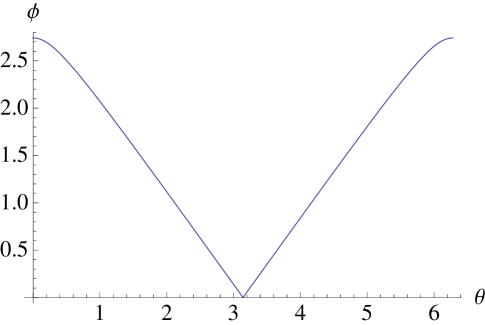
Figure 6: A plot of the eigen-phase $\phi$ against $\theta$ for the case $D_{1}=D_{2}=\pi/2-.2$. We are enforcing the condition $0\leq\phi\leq\pi$ that is required by our Bogoliubov transformation.

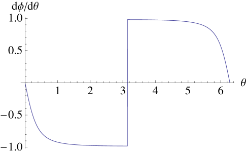
Figure 7: A plot of $d\phi/d\theta$ for $D_{1}=D_{2}=\pi/2-.2$

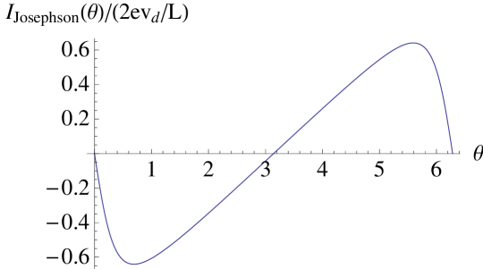
Figure 8: A plot of $I_{\rm Josephson}/(2ev_{d}/L)$ against $\theta$ for $D_{1}=D_{2}=\pi/2-.2$. Observe how the discontinuities combine to give a smooth result. As $D_{1,2}$ approach “perfect coupling” at $D_{1}=D_{2}=\pi/2$, the drops at $\theta=0,2\pi$ steepen, and become level-crossing discontinuities.

To gain further insight, consider the case of “perfect coupling,” where $\sin D_{a}=1$ and $\phi=\pm(\theta_{2}-\theta_{1}+\pi)$. In this case

$$U = \left[\matrix{0&-ie^{i\theta_{2}}\cr-ie^{-i\theta_{2}}&0}\right]\left[\matrix{0&-ie^{i\theta_{1}}\cr-ie^{-i\theta_{1}}&0}\right]$$ (33)

$$= \left[\matrix{-e^{i(\theta_{2}-\theta_{1})}&0\cr 0&-e^{-i(\theta_{2}-\theta_{1})}}\right],$$

and so $\phi=(\theta_{2}-\theta_{1})+\pi$. In the absence of relaxation, each $2\pi$ turn of $\theta$ would put another particle into both the spin-up and spin down sea. In equilibrium however, the state ceases to be occupied as soon at its energy becomes positive. This change in occupation leads to a jump in the Josephson current as the state crosses the Fermi energy and its contribution is lost. The maximum possible current occurs just before or after the jump, and has $I_{\rm max}=\pm 2ev_{d}/L$. For $v_{d}\sim 10^{6}\,{\rm m/s}$ and a perimeter of about $1\,{\rm mm}$ we get an upper bound on the Josephson current of about $1\,{\rm nA}$. This is consistent with the estimate of Ma and Zyuzin [11].

A physical picture for this upper bound is as follows: At the phase difference corresponding to the “jump,” we have a spin-up/spin-down pair of levels lying exactly at the Fermi energy. At perfect coupling, the extreme equilibrium currents correspond to two possible cases: i) between the leads both zero-energy levels are empty whilst outside they are occupied, ii) between the leads both zero-energy levels are occupied and outside they are empty. Levels in the Dirac sea that are not at the Fermi energy cannot be left empty by a passage under a lead, as this would lead to the energy being different in different regions and this is not possible in an energy eigenstate. Only the topmost energy level can contribute to the equilibrium Josephson current therefore, and this is the reason why the Josephson current is so small. To estimate its magnitude we note that in case (i), in each passage round the perimeter of the Hall bar, a pair of electrons passes from the Hall bar to the first lead and is returned to the Hall bar from the second lead. In case (ii) in each orbit a pair of electron passes from the first lead to the Hall bar, and is collected from the Hall bar at the second lead. This physical picture shows that the two possible Josephson currents are equal and opposite and have magnitude $|I_{\rm max}|=2ev_{d}/L$. (Because it is easy to get confused by Bogoliubov transformations, we provide, in Appendix A, a more detailed description of what happens to the particle content of the many-body eigenstates as they pass under the superconducting leads.)

IV Comparison with perturbation theory

The analytic regularization method used in the computations in the previous sections is standard in relativistic field theory [14], but is perhaps less familiar in superconducting applications. As a check on its validity it is worthwhile (and non-trivial) to compare our all-orders in $D_{1}$ and $D_{2}$ calculation with conventional perturbation theory.

In the weak-coupling regime, where $D_{1}$ and $D_{2}$ are small, the spherical cosine rule reduces to

$$\phi^{2}=D_{1}^{2}+D_{2}^{2}+2D_{1}D_{2}\cos\theta+O(D^{3}).$$ (34)

In this limit the ground-state energy and zero-temperature and Josephson current become

$$E_{\rm ground}(\theta)={v_{d}\over L}{1\over 2\pi}(D_{1}^{2}+D_{2}^{2}+2D_{1}D_{2}\cos\theta),$$ (35)

and hence

$$I_{\rm Josephson}=-{2ev_{d}\over\pi L}D_{1}D_{2}\sin\theta.$$ (36)

We begin by verifying that (35) is correctly reproduced by the perturbation expansion.

The Euclidean chiral propagator for zero temperature and anti-periodic spatial boundary conditions is

$${\langle 0|T\psi^{\dagger}_{a}(z_{1})\psi_{b}(z_{2})|0\rangle}=\delta_{ab}G(z_{1}-z_{2})={1\over 2iL}{\delta_{ab}\over\sin[\pi(z_{1}-z_{2})/L]}$$ (37)

where $a,b=\uparrow,\downarrow$ and $z=x+iv_{d}\tau$. The change in the $\Delta=0$ ground-state energy due to the interaction

$$H_{\rm int}=\int|\Delta(x)|\left(e^{i\theta(x)}\psi^{\dagger}_{\uparrow}(x)\psi^{\dagger}_{\downarrow}(x)+e^{-i\theta(x)}\psi_{\downarrow}(x)\psi_{\uparrow}(x)\right)dx$$ (38)

occurs at second order in $|\Delta|$, and is

$$\delta E_{\rm ground}=-\int dx_{1}\int dx_{2}\int_{-\infty}^{\infty}d\tau|\Delta(x_{1})||\Delta(x_{2})|e^{\theta(x_{1})}e^{-i\theta(x_{2})}{\langle 0|T\psi^{\dagger}_{\uparrow}(z_{1})\psi^{\dagger}_{\downarrow}(z_{1})\psi_{\downarrow}(z_{2})\psi_{\uparrow}(z_{2})|0\rangle}.$$ (39)

Here $\tau=\tau_{2}-\tau_{1}$ is the Euclidean time interval between $z_{2}$ and $z_{1}$. Now

$${\langle 0|T\psi^{\dagger}_{\uparrow}(z_{1})\psi^{\dagger}_{\downarrow}(z_{1})\psi_{\downarrow}(z_{2})\psi_{\uparrow}(z_{2})|0\rangle}=[G(z_{1}-z_{2})]^{2}$$ (40)

by Wick’s theorem, and

$${1\over 4L^{2}}\int_{-\infty}^{\infty}{1\over(\sin[\pi(x_{1}-x_{2}+iv_{d}\tau)/L])^{2}}\,d\tau=\left({1\over 2\pi Lv_{d}}\right)$$ (41)

is independent of the separation $x_{1}-x_{2}$ unless $x_{1}-x_{2}=0$ (mod $L$). The perturbation integral has four contributing regions: i) both $x_{1}$ and $x_{2}$ in lead 1, ii) both $x_{1}$ and $x_{2}$ in lead 2, iii) $x_{1}$ in lead 1, $x_{2}$ in lead 2, iv) $x_{1}$ in lead 2, $x_{2}$ in lead 1. Recalling that $D_{a}=|\Delta|w_{a}/v_{d}$, these combine to give

$$\delta E_{\rm ground} = v_{d}^{2}(D_{1}^{2}+D_{2}^{2}+2D_{1}D_{2}\cos\theta){1\over 2\pi Lv_{d}}$$ (42)

$$= {v_{d}\over 2\pi L}(D_{1}^{2}+D_{2}^{2}+2D_{1}D_{2}\cos\theta).$$

This expression coincides with the weak coupling limit of the all-orders calculation.

We can extend the comparison to non-zero temperature. At temperature $T=\beta^{-1}$, the Josephson current can be written as

$$I_{\rm Josephson}=\left({2e\over\hbar}\right){dF\over d\theta}$$ (43)

where $F$ is the free energy. For a general spectral shift $\phi$, we use standard methods to write down the partition function

$$Z = \exp\left\{-\beta F[\phi,\beta]\right\}$$ (44)

$$= \exp\left\{-{\beta v_{d}\over L}\left({\phi^{2}\over 2\pi}-{\pi\over 6}\right)\right\}\prod_{N=1}^{\infty}(1+wq^{2n-1})^{2}(1+w^{-1}q^{2n-1})^{2}$$

$$= (\eta(q))^{-2}\left[\sum_{n=-\infty}^{\infty}\exp\left\{-{v_{d}\beta\over 2\pi L}{1\over 2}\left(2\pi n+\phi\right)^{2}\right\}\right]^{2},$$

where $q=\exp\{-\pi\beta v_{d}/L\}$, $w=\exp\{-\beta v_{d}\phi/L\}$, and

$$\eta(q)=q^{1/12}\prod_{n=1}^{\infty}(1-q^{2n})$$

is the Dedekind eta function. We used the Jacobi triple-product formula to pass from the second line to the third. The sum in the expression for $Z$ is squared because there are two independent Fermi seas (spin up and spin down) and their contributions to the partition function are symmetric under the interchange of $\phi$ with $-\phi$. By using the Poisson summation formula, we can rewrite the partition function as

$$\exp\left\{-\beta F[\phi,\beta]\right\} = (\eta(q))^{-2}{L\over v_{d}\beta}\left[\sum_{n=-\infty}^{\infty}\exp\left\{-{1\over 2}{2\pi L\over v_{d}\beta}n^{2}+in\phi\right\}\right]^{2}$$ (45)

$$= (\eta(q))^{-2}{L\over v_{d}\beta}\left[\theta_{3}(\phi/2\pi|iL/v_{d}\beta)\right]^{2}$$

Thus the free energy is given by

$$F[\phi,\beta]=c-{2\over\beta}\ln\theta_{3}(\phi/2\pi|iL/v_{d}\beta).$$ (46)

where $c$ does not depend on $\phi$. For small spectral shifts $\phi$, we can Taylor expand

$$F[\phi,\beta]=c-{1\over\beta}\phi^{2}{d^{2}\over d\phi^{2}}\ln\theta_{3}(\phi/2\pi|L/v_{d}\beta)+O(\phi^{4}).$$ (47)

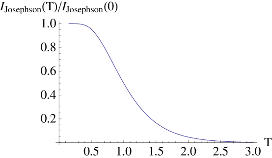
Figure 9: A plot of the effect of temperature on the perturbative Josephson current.. The horizontal axis is temperature in units of $\hbar v_{d}/L$. We see an effect as soon as the temperature becomes comparable with the $2\pi\hbar v_{d}/L$ level spacing of the edge energy states.

We would now like to compare the expression (47) with that obtained by perturbation theory. At finite temperature the chiral propagator becomes

$${\langle 0|T\psi^{\dagger}_{a}(z)\psi_{b}(0)|0\rangle}\to G(z)={1\over 2\pi iL}{\theta^{\prime}(0|iv_{d}\beta/L)\over\theta(z/L|iv_{d}\beta/L)}{\theta_{3}(z/L|iv_{d}\beta/L)\over\theta_{3}(0|iv_{d}\beta/L)}.$$ (48)

Here we are using the theta function definitions from [18], in which

$$\theta(z|\tau) = \sum_{m=-\infty}^{\infty}\exp\left\{i\pi\tau(m+1/2)^{2}+2\pi i(m+1/2)(z+1/2)\right\},$$

$$\theta_{3}(z|\tau) = \sum_{m=-\infty}^{\infty}\exp\left\{i\pi\tau m^{2}+2\pi imz\right\}.$$ (49)

Thus $\theta(z|\tau)$ is odd under $z\leftrightarrow-z$, while $\theta_{3}(z|\tau)$ is even. These properties were the ingredients used to assemble (48), which is specified uniquely by requiring the propagator to be analytic, doubly anti-periodic

$$G(z+L)=-G(z),\quad G(z+iv_{d}\beta)=-G(z),$$ (50)

and for small $z$ to obey

$$G(z)\sim{1\over 2\pi i}{1\over z}.$$ (51)

It is this last property that makes it a Green function.

In terms of $G(z)$ we now have

$$\delta E_{\rm ground}=-\int dx_{1}\int dx_{2}\int_{0}^{\beta}d\tau|\Delta(x_{1})||\Delta(x_{2})|e^{\theta(x_{1})}e^{-i\theta(x_{2})}[G(x_{1}-x_{2}+iv_{d}\tau)]^{2}.$$ (52)

The $x_{a}$ integrals are the same as before, and, although it is little more complicated, the integral over $\tau$ can still be evaluated in closed form. We begin by observing that $[2\pi iG(z)]^{2}$ is analytic, has a double pole $1/z^{2}$ at the origin, is doubly periodic with periods $\omega_{1}=L$ and $\omega_{2}=iv_{d}\beta$, and (from the $\theta_{3}(z|\tau)$ in the numerator) has a double zero at $z={1\over 2}(\omega_{1}+\omega_{2})$. These properties are sufficient to show that

$$[2\pi iG(z)]^{2}=\wp(z\,|\,\omega_{1},\omega_{2})-e_{3},$$ (53)

where $\wp(z\,|\,\omega_{1},\omega_{2})$ is the Weierstrass elliptic function, and

$$e_{3}\equiv\wp(\{\omega_{1}+\omega_{2}\}/2\,|\,\omega_{1},\omega_{1}).$$ (54)

The Weierstrass zeta function is defined so that

$${d\over dz}\zeta(z\,|\,\omega_{1},\omega_{2})=-\wp(z\,|\,\omega_{1},\omega_{2}),$$ (55)

together with initial condition

$$\lim_{z\to 0}\left\{\zeta(z)-{1\over z}\right\}=0.$$ (56)

We may therefore evaluate the $\tau$ integral in terms of tabulated functions:

$$\int_{a}^{a+\omega_{2}}[2\pi iG(z)]^{2}dz = -\zeta(a+\omega_{2})+\zeta(a)-\omega_{2}e_{3}$$ (57)

$$= -2\eta_{2}-\omega_{2}e_{3},$$

$$= \left.{1\over\omega_{2}}{d^{2}\over dz^{2}}\ln\theta_{3}(z|-\omega_{1}/\omega_{2})\right|_{z=0}.$$

Here $2\eta_{2}\equiv\zeta(a+\omega_{2})-\zeta(a)=2\zeta(\omega_{2}/2)$ is independent of $a$. The quantities in the second line of (57) are available in Mathematica™, and we use them to plot $I_{\rm Josephson}(T)/I_{\rm Josephson}(0)$ in Figure 9.

It takes a little more work to obtain the logarithmic derivative appearing in the last line of (57), and so we relegate its derivation to Appendix B. Accepting that the claim is correct, and putting in the dimensionful constants, we confirm that our all-orders evaluation of the free energy coincides with the perturbation theory calculation in the weak coupling regime .

V Discussion

We have shown that the maximum possible Josephson current for a pair of spin-up/spin-down QH edge states is rather small for typical Hall bar geometries. The bound is small because the relevant length and energy scales are set by the perimeter of the Hall device rather than the separation of the superconducting probes. Also, unlike a typical Josephson device, there is only one conduction channel per pair of edge modes. This last observation means that nothing is to be gained by making the superconducting leads overlay deeper into the Hall bar.

It may seem strange that we have so far discussed quantum Hall physics with no mention of the magnetic field that is necessary for its existence. The field, however, has only a few consequences for our discussion. Obviously the superconducting leads must be constructed of materials that remain superconducting in a field of few Tesla at temperatures of about 1K, but this is not hard to achieve. The leads must also be narrow enough that the order-parameter phase does not vary widely within the part of the lead that is actively coupled to the 2DEG. A subtle point in this regard affects the claim that the Josephson current is independent of the separation of the leads. The phase difference $\theta$ that we have equated to $\theta_{2}-\theta_{1}$ should be understood as the gauge invariant quantity $\theta=\theta_{2}-\theta_{1}-2e\int_{x_{1}}^{x_{2}}A\,dx$. Now a quantum of magnetic flux lies between each of the edge-state energy levels and if the effective “$\theta$” is not to vary with the energy level index $n$, only a small fraction of this flux should pass between the leads. The leads should not be spaced apart by more than a small fraction of the perimeter.

An effect that we have not considered here, and one that may well allow for larger currents, is “edge reconstruction” [20, 21, 22]. A reconstructed edge, with its alternating strips of compressible and incompressible 2DEG can allow many more levels to lie exactly at the fermi energy and so have their occupation number changed without a change in energy. These levels have zero drift velocity, however, so it unlikely that they contribute significantly to the Josephson current.

VI Acknowledgements

We thank Tony Leggett for interesting us the problem, and also Jim Eckstein and Stephanie Law Toner for explaining their work on QHE superconductor interfaces. The contribution of MS to this project was supported by the National Science Foundation under grant DMR 09-03291. The work of YL was supported by the US Department of Energy, Division of Materials Sciences, under award DE-FG02-07ER46453, admistered through the Frederick Seitz Materials Research Laboratory at the University of Illinois.

VII Appendix A

The maximum possible Josephson current occurs when we have both perfect coupling ($\sin D_{1}=\sin D_{2}=1$) and $\cos\theta=1$. In this special case we have

$$U_{1}=U_{2}=\left[\matrix{0&-i\cr-i&0}\right],\quad U=U_{2}U_{1}=-\left[\matrix{1&0\cr 0&1}\right].$$ (58)

The Bogoliubov mode-expansion (13) then becomes

$$\left(\matrix{\psi_{\uparrow}(x)\cr\psi^{\dagger}_{\downarrow}(x)}\right)=\sum_{n=-\infty}^{\infty}\left\{b_{n\uparrow}{1\over\sqrt{L}}\left(\matrix{1\cr 0}\right)e^{2\pi inx/L}+b^{\dagger}_{n\downarrow}{1\over\sqrt{L}}\left(\matrix{0\cr 1}\right)e^{-2\pi inx/L}\right\}$$ (59)

for $x$ in region (1), and

$$\left(\matrix{\psi_{\uparrow}(x)\cr\psi^{\dagger}_{\downarrow}(x)}\right)=\sum_{n=-\infty}^{\infty}\left\{b_{n\uparrow}{1\over\sqrt{L}}\left(\matrix{0\cr-i}\right)e^{2\pi inx/L}+b^{\dagger}_{n\downarrow}{1\over\sqrt{L}}\left(\matrix{-i\cr 0}\right)e^{-2\pi inx/L}\right\}$$ (60)

for $x$ in region (2). (The numbering of the regions refers to figure 1.)

In these mode-expansions, the operators $b_{n\uparrow}$ and $b^{\dagger}_{n\downarrow}$ annihilate or create quasiparticles with energy $|E_{n}|=2\pi v_{d}|n|/L$. We compare these expansions with the free-particle plane wave expansion

$$\left(\matrix{\psi_{\uparrow}(x)\cr\psi^{\dagger}_{\downarrow}(x)}\right)=\sum_{n=-\infty}^{\infty}\left\{a_{n\uparrow}{1\over\sqrt{L}}\left(\matrix{1\cr 0}\right)e^{2\pi inx/L}+a^{\dagger}_{n\downarrow}{1\over\sqrt{L}}\left(\matrix{0\cr 1}\right)e^{-2\pi inx/L}\right\},$$ (61)

where the operators $a_{n\uparrow}$ and $a^{\dagger}_{n\downarrow}$ annihilate and create electrons. We see that we can identify

$$b_{n\uparrow}=a_{n\uparrow}, b^{\dagger}_{n\uparrow}=a^{\dagger}_{n\uparrow}$$

$$b_{n\downarrow}=a_{n\downarrow}, b^{\dagger}_{n\downarrow}=a^{\dagger}_{n\downarrow}$$ (62)

in region (1), and

$$b_{n\uparrow}=ia^{\dagger}_{-n\downarrow}, b^{\dagger}_{n\uparrow}=-ia_{-n\downarrow}$$

$$b_{n\downarrow}=-ia^{\dagger}_{n\downarrow}, b^{\dagger}_{n\downarrow}=+ia_{-n\uparrow}$$ (63)

in region (2). We now use these identifications to examine what happens to the particle content of the many-body eigenstates as they drift under the superconducting leads.

We first note a minimum-energy eigenstate must be annihilated by $b_{n\uparrow}$ and $b_{n\downarrow}$ for $n>0$, and by $b^{\dagger}_{n\uparrow}$ and $b^{\dagger}_{n\downarrow}$ for $n<0$. Let us define the eigenstate ${|0\rangle}$ by requiring that it is killed by all these operators, and also by $b_{0\downarrow}$ and $b_{0\uparrow}$. Then the states

$${|0\rangle},\quad b^{\dagger}_{0\uparrow}{|0\rangle},\quad b^{\dagger}_{0\downarrow}{|0\rangle},\quad b^{\dagger}_{0\downarrow}b^{\dagger}_{0\uparrow}{|0\rangle},$$ (64)

all have the same energy, making the ground state four-fold degenerate.

With the operator identifications established above, we find that

$${|0\rangle}=\prod_{n=-\infty}^{-1}(a^{\dagger}_{n\downarrow}a^{\dagger}_{n\uparrow}){|\rm empty\rangle}$$ (65)

when $x$ lies in region (1), but in region (2), where $b_{0\uparrow}$ and $b_{0\downarrow}$ are identified with $a^{\dagger}_{0\downarrow}$ and $a^{\dagger}_{0\uparrow}$ respectively, we must have

$${|0\rangle}\propto a^{\dagger}_{0\downarrow}a^{\dagger}_{0\uparrow}\prod_{n=-\infty}^{-1}(a^{\dagger}_{n\downarrow}a^{\dagger}_{n\uparrow}){|\rm empty\rangle},$$ (66)

for it still to be annihilated by $b_{0\uparrow}$ and $b_{0\downarrow}$. We see that the occupation number of the energy levels for $n<0$ are unchanged, but ${|0\rangle}$ picks up a pair of $n=0$ electrons from the superconducting lead as it passes under it. Similarly the state $b^{\dagger}_{0\downarrow}b^{\dagger}_{0\uparrow}{|0\rangle}$ loses a pair from the $n=0$ level.

The state $b^{\dagger}_{0\uparrow}{|0\rangle}$ is annihilated by $a^{\dagger}_{0\uparrow}$ and $a_{0\downarrow}$ in region (1), and these become respectively $a_{0\downarrow}$ and $a^{\dagger}_{0\uparrow}$ in region (2). The particle content of this state is unaffected by its passage under the lead therefore. Similarly $b^{\dagger}_{0\downarrow}{|0\rangle}$ retains its particle content.

Now consider an excited state, for example $b^{\dagger}_{m\uparrow}b^{\dagger}_{0\uparrow}{|0\rangle}$ with $m>0$. This state has energy $E=2\pi v_{d}m/L$. In region (1) it has particle content

$$a^{\dagger}_{m\uparrow}a^{\dagger}_{0\uparrow}\prod_{n=-\infty}^{-1}(a^{\dagger}_{n\downarrow}a^{\dagger}_{n\uparrow}){|\rm empty\rangle},$$ (67)

and so consists of a Dirac sea together with an electron in a positive energy level. In region (2) it becomes

$$a_{-m\downarrow}a^{\dagger}_{0\uparrow}\prod_{n=-\infty}^{-1}(a^{\dagger}_{n\downarrow}a^{\dagger}_{n\uparrow}){|\rm empty\rangle},$$ (68)

which consists of a Dirac sea which has lost an electron from a negative energy level. After passing the superconductor therefore, the state has the same energy and spin, but the electron has become a hole.

VIII Appendix B

We wish to establish the third line of (57), which reads

$$\int_{a}^{a+\omega_{2}}(\wp(z|\omega_{1},\omega_{2})-e_{3})dz=\left.{1\over\omega_{2}}{d^{2}\over dz^{2}}\ln\theta_{3}(z|-\omega_{1}/\omega_{2})\right|_{z=0}.$$ (69)

This result follows indirectly from the related integral

$$\int_{a}^{a+\omega_{1}}\left\{\wp(z|\omega_{1},\omega_{2})-e_{3}\right\}dz = -2\eta_{1}-\omega_{1}e_{3}$$ (70)

$$= {1\over\omega_{1}}{\theta^{\prime\prime}_{3}(0|\omega_{2}/\omega 1)\over\theta_{3}(0|\omega_{2}/\omega_{1})},$$

$$= \left.{1\over\omega_{1}}{d^{2}\over dz^{2}}\ln\theta_{3}(z|\omega_{2}/\omega_{1})\right|_{z=0}.$$

Here we require ${\rm Im\,}(\omega_{2}/\omega_{1})>0$ for the theta functions to converge. To establish (70) we observe that second line follows from the first by combining two standard formulæ:

$$e_{3}={1\over\omega_{1}^{2}}\left\{{1\over 3}{\theta^{\prime\prime\prime}(0|\tau)\over\theta^{\prime}(0|\tau)}-{\theta^{\prime\prime}_{3}(0|\tau)\over\theta_{3}(0|\tau)}\right\},$$ (71)

([18] Eq 5.2), and

$$2\eta_{1}=-{1\over\omega_{1}}{1\over 3}{\theta^{\prime\prime\prime}(0|\tau)\over\theta^{\prime}(0|\tau)},$$ (72)

([19] §21.43.) Here $\tau=\omega_{2}/\omega_{1}$ with ${\rm Im\,}\tau>0$. The third line of (70) follows from the second because $\theta_{3}^{\prime}(0|\tau)=0$.

To derive (69) however, we need the integral over the $\omega_{2}=iv_{d}\beta$ imaginary period, and not over the $\omega_{1}=L$ real period. Because of the positivity condition on the imaginary part of $\tau$, we cannot change the integration path by merely interchanging $\omega_{1}\leftrightarrow\omega_{2}$ in equation (70). We need to be more subtle. By changing $(\omega_{1},\omega_{2})\to(-\omega_{2},\omega_{1})$ in (70), we obtain

$$-\left.{1\over\omega_{2}}{d^{2}\over dz^{2}}\ln\theta_{3}(z|-\omega_{1}/\omega_{2})\right|_{z=0}=\int_{a}^{a-\omega_{2}}\left\{\wp(z|-\omega_{2},\omega_{1})-e_{3}\right\}dz.$$ (73)

This last equation is legitimate because ${\rm Im\,}(\omega_{2}/\omega_{1})>0$ implies that ${\rm Im\,}(-\omega_{1}/\omega_{2})>0$. We now manipulate

$$RHS = -\int_{a}^{a+\omega_{2}}\left\{\wp(z|-\omega_{2},\omega_{1})-e_{3}\right\}dz$$ (74)

$$= -\int_{a}^{a+\omega_{2}}\left\{\wp(z|\,\omega_{1},\omega_{2})-e_{3}\right\}dz,$$

where the last line follows from the invariance of $\wp(z|\,\omega_{1},\omega_{2})$ under modular transformations

$$\left(\matrix{\omega_{1}^{\prime}\cr\omega_{2}^{\prime}}\right)=\left(\matrix{a&b\cr c&d}\right)\left(\matrix{\omega_{1}\cr\omega_{2}}\right),\qquad\left(\matrix{a&b\cr c&d}\right)\in{\rm SL}(2,{\mathbb{Z}}).$$ (75)

From this we immediately deduce eq. (69).