Quantum Faraday Effect in Double-Dot Aharonov-Bohm Ring

Abstract

We investigate Faraday’s law of induction manifested in the quantum state of Aharonov-Bohm loops. In particular, we propose a flux-switching experiment for a double-dot AB ring to verify the phase shift induced by Faraday’s law. We show that the induced Faraday phase is geometric and nontopological. Our study demonstrates that the relation between the local phases of a ring at different fluxes is not arbitrary but is instead determined by Faraday’s inductive law, which is in strong contrast to the arbitrary local phase of an Aharonov-Bohm ring for a given flux.

We begin by pointing out an apparent paradox between the two well known facts in quantum theory: (1) the local phase factor of the wave function in an Aharonov-Bohm (AB) loop is arbitrary gasiorowicz ; (2) the wave function (more generally, the density matrix) of a quantum system can be reconstructed by a technique of the quantum state tomography (QST) on repeated preparation of the system vogel89 ; paris04 . Aharonov-Bohm (AB) effect aharonov59 is one of the most striking phenomena discovered in quantum theory. In the case of an arbitrary AB loop at equilibrium, any physical quantity is periodic in $\Phi$ with a period $\Phi_{0}=e/hc$, the flux quantum (“Byers-Yang’s theorem”) byers61 . AB effect is gauge-invariant and appears as a manifestation of the gauge-invariant phase factor. The choice of a particular gauge is arbitrary, and therefore the local phase factor of the wave function is also arbitrary.

It is interesting to note that this arbitrary local phase factor of an AB loop is inconsistent with the fact that the wave function can be reconstructed by the technique of QST. The gap between the two facts needs to be clarified. In this Letter, we show that the law of Faraday’s induction plays a central role when we try to reconstruct the wave function of an AB loop. For a full reconstruction of the wave function, change of the AB flux is inevitable. The change of the AB flux results in Faraday’s induction, and gives rise to an additional phase shift. We find that this Faraday-induced phase shift is geometric and nontopological. It is geometric in the sense that it depends only on the net change of the magnetic field. On the other hand, it is nontopological since it depends not only on the flux change but also on the specific geometry of the system.

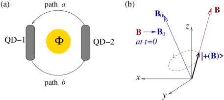
Figure 1: (Color online) (a) Schematic of an Aharonov-Bohm ring composed of two quantum dots. (b) Illustration of the state evolution $|\psi_{\phi\rightarrow 0}(t)\rangle$ in the Bloch-sphere representation after a sudden drop in the AB flux.

We analyze the characteristics of the quantum Faraday effect for a tunnel-coupled double-dot AB loop with a localized magnetic flux $\Phi$ penetrating the hole (Fig. 1(a)). This is the simplest two-state problem involving an AB flux. The Hamiltonian of a double-dot loop is given by

$$H=\sum_{\alpha=1,2}\varepsilon_{\alpha}c_{\alpha}^{\dagger}c_{\alpha}-(te^{i\phi_{a}}c_{1}^{\dagger}c_{2}+te^{i\phi_{b}}c_{2}^{\dagger}c_{1})-\mbox{h.c.},$$ (1a)

where $$c_{\alpha} c_{\alpha}^{\dagger} \alpha \alpha=1,2 \varepsilon_{\alpha} t a b \phi =2\pi\Phi/\Phi_{0} \phi=\phi_{a}+\phi_{b} \phi_{a} \phi_{b} \phi$$() annihilates(creates) an electron at QD- () with its energy level . For simplicity, tunneling amplitude is assumed to be identical for both the upper (path ) and the lower (path ) paths. The AB phase () is given by . The “local” phases and are not gauge-invariant. Only is a gauge-invariant phase. This Hamiltonian can be simplified as

$$H=\sum_{\alpha=1,2}\varepsilon_{\alpha}c_{\alpha}^{\dagger}c_{\alpha}+t_{\phi}c_{1}^{\dagger}c_{2}+t^{*}_{\phi}c_{2}^{\dagger}c_{1},$$ (1b)

with the effective tunneling amplitude

$$t_{\phi}=-2te^{i(\phi_{a}-\phi_{b})}\cos{(\phi/2)}\,.$$ (1c)

Note that $t_{\phi}$ depends on the choice of gauge due to the phase factor $e^{i(\phi_{a}-\phi_{b})}$.

It is useful to rewrite the Hamiltonian (Eq. 1) in a Bloch-sphere (pseudospin) representation with $|\uparrow\rangle=|1\rangle$ and $|\downarrow\rangle=|2\rangle$:

$$H=-\frac{1}{2}\vec{\sigma}\cdot\mathbf{B},$$ (2a)

where

$$\mathbf{B}=(-2\mbox{\rm Re}(t_{\phi}),2\mbox{\rm Im}(t_{\phi}),\Delta\varepsilon)$$ (2b)

is a pseudo-magnetic field, and $\vec{\sigma}=(\sigma_{x},\sigma_{y},\sigma_{z})$. $\Delta\varepsilon=\varepsilon_{2}-\varepsilon_{1}$ is the energy level detuning of the two dots. We imposed the condition $\varepsilon_{1}+\varepsilon_{2}=0$ without loss of generality.

It is straightforward to obtain the eigenstate energies and the corresponding eigenvectors. Although a multi-valued wave function cannot be ruled out a priori byers61 , we do not consider this possibility because a QST with multi-valued wave function is meaningless merzbacher62 . The two eigenstate energies are $E_{\pm}(\mathbf{B})=\mp\frac{1}{2}|\mathbf{B}|=\mp\frac{1}{2}\sqrt{(\Delta\varepsilon)^{2}+4|t_{\phi}|^{2}}$, with the corresponding eigenvectors being given by

$$|\pm(\mathbf{B})\rangle=\alpha_{\pm}|\uparrow\rangle+\beta_{\pm}|\downarrow\rangle,$$ (3a)

where

$$\alpha_{\pm}=\frac{t_{\phi}}{\sqrt{(\varepsilon_{1}-E_{\pm})^{2}+|t_{\phi}|^{2}}},\;\beta_{\pm}=-\frac{\varepsilon_{1}-E_{\pm}}{\sqrt{(\varepsilon_{1}-E_{\pm})^{2}+|t_{\phi}|^{2}}}.$$ (3b)

Although the energy eigenvalue $E_{\pm}$ is periodic in the AB phase $\phi$ with a period of $2\pi$ (as indicated by Byers-Yang’s theorem byers61 ), the wave function does not show such periodicity. Instead, the wave function depends on the arbitrary choice of the phases $\phi_{a}$ and $\phi_{b}$. This is evident from the gauge-dependent factor $t_{\phi}$ in Eq. (3b) (see also Eq. (1c)).

Now, let us discuss the following flux-switching and pseudospin precession experiment (see also the illustration of Fig. 1(b)). This kind of time-domain experiment is an essential part of a QST with a system involving an AB flux liu05 . Initially, the AB flux is prepared to have an arbitrary, fixed value $\phi$, and the system is in the ground state $|+(\mathbf{B})\rangle$ of Eq. (3). It is assumed that thermal fluctuations are small enough that the system is in the ground state, that is, $k_{B}T\ll|\mathbf{B}|$. Then, the external magnetic flux is suddenly dropped to zero, and the pseudo-magnetic field $\mathbf{B}$ changes immediately to the value given by Eq. (2b) with $\phi=0$ and $\phi_{b}=0$. ($\phi_{b}$ might be chosen to be nonzero in general, but it does not make any change to our findings here.) This corresponds to

$$\mathbf{B}\rightarrow\mathbf{B}_{0}=(4t,0,\Delta\varepsilon).$$ (4)

Because of the sudden change in $\mathbf{B}$, the state of the electron, denoted by $|\psi_{\phi\rightarrow 0}(t)\rangle$, will precess according to the relation (shown as a dashed line in Fig. 1(b)) $|\psi_{\phi\rightarrow 0}(t)\rangle=e^{\frac{i}{2}\vec{\sigma}\cdot\hat{n}B_{0}t}|+(\mathbf{B})\rangle$, where $\hat{n}$ is the unit vector parallel to $\mathbf{B}_{0}$, and $B_{0}$ is its magnitude. We obtain

$$|\psi_{\phi\rightarrow 0}(t)\rangle=\alpha_{0}(t)|\uparrow\rangle+\beta_{0}(t)|\downarrow\rangle,$$ (5a)

where

$$\alpha_{0}(t) = \alpha_{+}\cos{\frac{B_{0}t}{2}}+i\left(\alpha_{+}n_{z}+\beta_{+}n_{x}\right)\sin{\frac{B_{0}t}{2}},$$ (5b)

$$\beta_{0}(t) = \beta_{+}\cos{\frac{B_{0}t}{2}}-i\left(\beta_{+}n_{z}-\alpha_{+}n_{x}\right)\sin{\frac{B_{0}t}{2}}.$$ (5c)

Here $n_{x}$($n_{z}$) is the $x$($z$) component of the vector $\hat{n}$.

The time evolution of the state, $|\psi_{\phi\rightarrow 0}(t)\rangle$, depends on the gauge, simply because $\mathbf{B}$ depends on the gauge. Furthermore, this gauge dependence is shown in physical quantities, for instance, in the time evolution of the electron number at QD-1 (or at QD-2):

$$n_{1}(t)=\langle\psi_{\phi\rightarrow 0}(t)|c_{1}^{\dagger}c_{1}|\psi_{\phi\rightarrow 0}(t)\rangle=|\alpha_{0}(t)|^{2}.$$ (6)

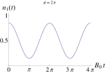
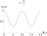
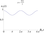
Figure 2: (Color online) Time dependence of the electron number at QD-1 ($n_{1}(t)$) for the symmetric gauge, upon a sudden drop in the AB phase from $\phi$ to zero. Six different input values of $\phi$ are used, and $\Delta\varepsilon=4t$ in all graphs.

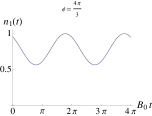
Figure 3: (Color online) Time dependence of the electron number at QD-1 ($n_{1}(t)$) for “$\phi_{b}=0$” gauge, upon a sudden drop in the AB phase from $\phi$ to zero. Three different input values of $\phi$ are used, and $\Delta\varepsilon=4t$ for all graphs.

The time evolution of $n_{1}$ is displayed for two different choices of gauge: (i) symmetric gauge ($\phi_{a}=\phi_{b}=\phi/2$) (Fig. 2), and (ii) “$\phi_{b}=0$” gauge (Fig. 3). (In fact, an infinite number of gauge choices exists which satisfy the condition $\phi_{a}+\phi_{b}=\phi$). For the symmetric gauge, the effective tunneling amplitude is $t_{\phi}=-2t\cos{(\phi/2)}$. This gauge leads to a $4\pi$-periodicity of the Hamiltonian and its eigenstates (Eqs. (1,3)). On the other hand, for the “$\phi_{b}=0$” gauge, $t_{\phi}=-t(e^{i\phi}+1)$, which provides a $2\pi$-periodicity of the Hamiltonian and its eigenstates. Obviously, a different choice of gauge leads to a different result.

Of course, the gauge dependence of the results shown in Fig. 2 and Fig. 3 should not exist in reality. The result should be unique in spite of the choice of gauge. In fact, the contradiction is resolved if we take into account Faraday’s law induction in the flux-switching procedure. When the localized magnetic field changes in time, the electric field

$$\mathbf{E}=-\nabla V-\frac{1}{c}\frac{\partial\mathbf{A}}{\partial t}$$ (7)

is induced, where $V$ and $\mathbf{A}$ are the scalar and the vector potentials, respectively. The choice of the gauges for $V$ and $\mathbf{A}$ should provide the correct value of $\mathbf{E}$, which was not taken into account in obtaining the results displayed Figs. 2 and 3. Still there is a freedom to choose the gauge, and we choose $V$ to be time-independent, and then the inductive component of the field, $\mathbf{E}_{t}$, is given by $\mathbf{E}_{t}=-\frac{1}{c}\frac{\partial\mathbf{A}}{\partial t}$. For the system under consideration, the following relations are derived from Faraday’s law:

$$\int_{\gamma}\mathbf{E}_{t}\cdot d\mathbf{R}=-\frac{1}{c}\frac{\partial}{\partial t}\int_{\gamma}\mathbf{A}\cdot d\mathbf{r}=-\frac{\hbar}{e}\frac{\partial\phi_{\gamma}}{\partial t},$$ (8)

where $\int_{\gamma}$ represents an integral over the path $\gamma$ ($a$ or $b$).

The question at this point is how to choose a gauge giving the correct inductive field. Actually, the induced electric field depends not only on the time-dependent flux $\Phi(t)$ but also on the specific geometry of the system and the distribution of the localized magnetic flux. Let us consider, for example, a highly symmetric double-dot ring: with circular symmetric AB flux and identical paths for the upper (path $a$) and the lower (path $b$) parts of the ring. Then, the symmetry of the system leads to the relation $\int_{a}\mathbf{E}_{t}\cdot d\mathbf{R}=\int_{b}\mathbf{E}_{t}\cdot d\mathbf{R}$, or $\frac{\partial\phi_{a}}{\partial t}=\frac{\partial\phi_{b}}{\partial t}$. We find that this condition is fulfilled by choosing the symmetric gauge for the time-dependent phases: $\phi_{a}(t)=\phi_{b}(t)=\phi(t)/2$. Therefore, the results shown in Fig. 2 are correct for the symmetric system because they give the correct value of $\mathbf{E}_{t}$. In general, the gauge should be selected to give the correct value of $\mathbf{E}_{t}$, which depends on the specific geometry of the system.

An important implication of the above discussion on Faraday’s induction is that it gives an additional local phase in the wave function of the system. In the following, we show that Faraday’s induction gives a geometrical (but nontopological) phase shift. Here we discuss it for a specific double-dot ring system, but it can be applied equally to any AB loops. The initial (local) phases at $t=t_{i}$ are represented by $\phi_{a}^{i}$ and $\phi_{b}^{i}$ for paths $a$ and $b$, respectively. These phases evolve as the magnetic field changes in time, and the final values (at $t=t_{f}$) are given by $\phi_{a}^{i}+\Delta\phi_{a}$ and $\phi_{b}^{i}+\Delta\phi_{b}$, respectively. During the change in the magnetic field, the inductive field induces a momentum kick $\Delta\mathbf{p}(\mathbf{r})$ which depends on the position $\mathbf{r}$ as

$$\Delta\mathbf{p}(\mathbf{r})=e\int_{t_{i}}^{t_{f}}\mathbf{E}_{t}\,dt=-\frac{e}{c}\Delta\mathbf{A}(\mathbf{r}),$$ (9)

where $\Delta\mathbf{A}(\mathbf{r})$ is the change in the vector potential. This momentum kick induces a local phase shift

$$\phi^{F}(\mathbf{r})=\frac{1}{\hbar}\Delta\mathbf{p}(\mathbf{r})\cdot\mathbf{r},$$ (10)

in the wave function. From this relation, one can find that Faraday’s induction gives the relative phases of the two quantum dots

$$\phi^{F}_{a}=\frac{1}{\hbar}\int_{a}\Delta\mathbf{p}(\mathbf{r})\cdot d\mathbf{r}=-\Delta\phi_{a},$$

for path $a$. Similarly, it gives $\phi^{F}_{b}=-\Delta\phi_{b}$ for path $b$. It is interesting to note that the Faraday phase for one loop is equivalent to the negative of the change in the AB phase: $\phi^{F}_{one\,loop}=\frac{1}{\hbar}\oint\Delta\mathbf{p}(\mathbf{r})\cdot d\mathbf{r}=-\Delta\phi$ . In contrast to the AB effect, not only the phase for one loop but also the local phase $\phi^{F}(\mathbf{r})$ is physically meaningful because the latter is directly related to the inductive field, a physical quantity. Note that, the local phase $\phi^{F}(\mathbf{r})$ is geometric in the sense that it depends only on the net change of the vector potential $\Delta\mathbf{A}(\mathbf{r})$. However, this phase is nontopological because it depends not only on the topology of the ring, but also on the specific geometry. The $4\pi$-periodicity of a symmetric double-dot ring can be understood from the $4\pi$-periodicity of the phases $\phi^{F}_{a}$ and $\phi^{F}_{b}$, since it satisfies

$$\phi^{F}_{a}=\phi^{F}_{b}=-\Delta\phi/2.$$ (11)

The effect of the Faraday phase can be observed even in an adiabatic change of the magnetic flux. Two conditions are necessary for this purpose. First, a nonstationary initial state should be prepared. Otherwise, the adiabatic evolution of the magnetic field gives just an adiabatic evolution of the ground state, and the Faraday phase is not observable. Second, the characteristic time scale of the flux change, denoted by $\Delta t$, should meet the condition $\hbar/|\mathbf{B}|\ll\Delta t\ll t_{deph}$, where $t_{deph}$ is the dephasing time of the initial nonstationary state. The flux should change at a much slower rate than the precession frequency of the pseudospin (adiabaticity), but should be switched faster than the dephasing time, in order to observe the evolution of the nonstationary state.

The procedure for a possible experiment is as follows: (i) a ground state is prepared with $\Delta\varepsilon=0$ and $\mathbf{B}=\mathbf{B}_{i}$. (ii) A nonstationary state is initialized by a sudden switching of the level detuning from zero to a finite value $\Delta\varepsilon$. (iii) The magnetic flux is adiabatically switched so that the pseudo-magnetic field $\mathbf{B}$ changes accordingly. (iv) Finally, the time evolution of the electron number is measured in one of the QDs.

The adiabatic process of (iii) is described by the Hamiltonian $H\{\mathbf{B}(t)\}=-\vec{\sigma}\cdot\mathbf{B}(t)/2$ with an adiabatic change of $\mathbf{B}$. The nonstationary initial state immediately after process (ii) (for a symmetric ring with the initial AB phase in the range of $\pi<\phi<3\pi$),

$$|\psi_{0}\rangle=\frac{1}{\sqrt{2}}\left(|\uparrow\rangle-|\downarrow\rangle\right),$$ (12a)

evolves upon the adiabatic change in $$\mathbf{B}(t)$$. It satisfies the adiabatic evolution of the eigenstates

$$|\psi_{\pm}(\mathbf{B}(t))\simeq e^{i\gamma_{\pm}(\mathbf{B})}e^{-i\int_{0}^{t}E_{\pm}(t^{\prime})dt^{\prime}}|\pm(\mathbf{B}(t)\rangle,$$ (12b)

where $$\gamma_{\pm} \mathbf{B}(t) \gamma_{\pm}=0 \phi_{a}(t)=\phi_{b}(t)$$ denotes the geometric phase acquired during the adiabatic change of  berry84 . We find that for the symmetric ring (imposed by the relation ). Therefore, the time evolution of the state upon adiabatic change is given by

$$|\psi(t)\rangle=c_{+}e^{i\phi^{+}_{dy}(t)}|+(\mathbf{B}(t))\rangle+c_{-}e^{i\phi^{-}_{dy}(t)}|-(\mathbf{B}(t))\rangle,$$ (12c)

where $$c_{\pm}=\langle\pm(\mathbf{B}_{i})|\psi_{0}\rangle$$, and

$$\phi^{\pm}_{dy}(t)\equiv-\int^{t}E_{\pm}(\mathbf{B}(t^{\prime}))dt^{\prime}=\pm\frac{1}{2}\int^{t}\mathbf{B}(t^{\prime})dt^{\prime}$$ (12d)

is a dynamical phase.

It is also useful to define the difference between the two dynamical phases, $\Delta\phi_{dy}(t)\equiv\phi^{+}_{dy}(t)-\phi^{-}_{dy}(t)$.

The time evolution of the electron number at QD-1 (state $|\uparrow\rangle$) is

$$n_{1}(t)=|\langle\uparrow|\psi(t)\rangle|^{2}\,.$$ (13)

We find from Eq. (12d) that

$$\langle\uparrow|\psi(t)\rangle=u(t)\cos{(\Delta\phi_{dy}(t)/2)}+iv(t)\sin{(\Delta\phi_{dy}(t)/2)},$$ (14a)

where

$$u(t) = \frac{1}{\sqrt{2}}\left(\cos{\frac{\theta_{i}-\theta(t)}{2}}-\sin{\frac{\theta_{i}-\theta(t)}{2}}\right),$$ (14b)

$$v(t) = \frac{1}{\sqrt{2}}\left(\cos{\frac{\theta_{i}+\theta(t)}{2}}-\sin{\frac{\theta_{i}+\theta(t)}{2}}\right).$$ (14c)

$\theta$($\theta_{i}$) is the angle between the $z$-axis and $\mathbf{B}$($\mathbf{B}_{i}$) in the Bloch sphere.

Fig. 4 displays the time evolution of the occupation number, $n_{1}$, as a function of $\Delta\phi_{dy}(t)$, for an adiabatic change in the AB phase of the form $\phi(t)=\frac{\phi_{i}}{2}\left[1-\tanh{(\eta\,\Delta\phi_{dy}(t))}\right]$. The initial phase $\phi=\phi_{i}$ at $\Delta\phi_{dy}(t)\ll-\eta^{-1}$ changes adiabatically to $\phi=0$ at $\Delta\phi_{dy}(t)\gg\eta^{-1}$. The parameter $\eta$ determines the rate of change. As discussed above, we have another condition $\phi_{a}(t)=\phi_{b}(t)=\phi(t)/2$ for a symmetric ring, which takes Faraday’s induction into account. The time evolution of $n_{1}$ for $\phi_{i}=2\pi$ with $\eta=0.04$ is plotted in Fig. 4 (solid line). This is compared to the case of the static AB phase, $\phi(t)=2\pi$ (dashed line). The result shows that the adiabatic change of the AB phase from $2\pi$ to zero indeed leads to out-of-phase oscillation of $n_{1}$. This shift of the phase in $n_{1}$ results from the Faraday phase, $\phi^{F}_{a}=\phi^{F}_{b}=-\Delta\phi/2=\pi$, as shown in Eq. (11). Note that the AB effect does not play any role when $\phi$ changes by $2\pi$.

The double-dot AB ring system is equivalent to a single Cooper pair box (SCB) composed of two Josephson junctions with an AB flux nakamura99 ; makhlin01 , if the two QD states are replaced by the two charge states in the SCB. The experiments described above can be applied equally to a SCB. It could be more easily realized with a SCB, considering the recent progress made in controlling superconducting qubits makhlin01 .

At this stage, we are able to address the question raised at the very beginning of this Letter: the inconsistency between the arbitrary local phase in an AB loop and the possibility of its measurement with a QST. Of course, a measurement of the local phase of a static AB ring is meaningless since it is arbitrary. However, for a complete QST, one should also change the localized AB flux. What is measured during a QST (which inevitably involves a change of the flux) is not an arbitrary local phase but the Faraday phase induced by the change in the flux itself.

In conclusion, we have shown that the relative local phase at different strengths of flux in an AB loop is not arbitrary but is instead determined by Faraday’s law of induction. This is in strong contrast to the arbitrary local phase factor of an AB loop which depends on the choice of gauge in the vector potential. Faraday’s induction provides a geometric and nontopological contributions to the local phase of a ring. Flux-switching experiments for double-dot rings have been proposed to verify the effect of the Faraday phase. Measurement of the Faraday phase in our setup of a double-dot ring is just one example of the very general nature of the problem. It should be observable in various different types of AB loops, which calls for further study.

This work was supported by National Research Foundation of Korea under Grant No. 2009-0072595 and No. 2009-0084606, and by LG Yeonam Foundation.

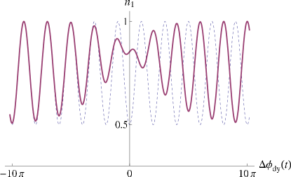
Figure 4: (Color online) Time dependence of $n_{1}$ upon an adiabatic change of the flux for a nonstationary initial state of Eq. (12a) (solid line). The parameters used here are $\Delta\varepsilon=0\rightarrow 4t$, $\phi_{i}=2\pi$, and $\eta=0.04$. For comparison, the time evolution of $n_{1}$ for a static AB phase ($\phi(t)=2\pi$) is also plotted (dashed line).

References

- (1) See e.g., S. Gasiorowicz, Quantum Physics, 3rd ed. (John Wiley & Sons, New Jersey, 2003).
- (2) K. Vogel and H. Risken, Phys. Rev. A40, R2847 (1989); U. Leonhardt, Phys. Rev. Lett. 74, 4101 (1995).
- (3) For a review, see e.g., Quantum State Estimation, ed., by M. Paris and J. Rehácek (Springer, Berlin, 2004).
- (4) Y. Aharonov and D. Bohm, Phys. Rev. 115, 485 (1959); ibid. 123, 1511 (1961).
- (5) N. Byers and C. N. Yang, Phys. Rev. Lett. 7, 46 (1961).
- (6) For a useful discussion on the single valuedness of the wave function, see e.g., E. Merzbacher, Am. J. Phys. 30, 237 (1962).
- (7) Y.-x. Liu, L. F. Wei, and F. Nori, Phys. Rev. B72, 014547 (2005).
- (8) M. V. Berry, Proc. R. Soc. London A 392, 45 (1984).
- (9) Y. Nakamura, Yu. A. Pashkin, and J. S. Tsai, Nature 398, 786 (1999).
- (10) For a review, see e.g., Y. Makhlin, G. Schön, and A. Shnirman, Rev. Mod. Phys. 73, 357 (2001); J. Clarke and F. K. Wilhelm, Nature 453, 1031 (2008).