Singular matrix Darboux transformations in the inverse scattering method

Abstract

Singular Darboux transformations, in contrast to the conventional ones, have a singular matrix as a coefficient before the derivative. We incorporated such transformations into a chain of conventional transformations and presented determinant formulas for the resulting action of the chain. A determinant representation of the Kohlhoff-von Geramb solution to the Marchenko equation is given.

1 Introduction

The idea to use Darboux (or equivalently supersymmetric, or simply SUSY) transformations for solving the inverse scattering problem for the one-dimensional one-channel Schrödinger equation was formulated in the most clear way by Sukumar [1]. It was essentially advanced by introducing phase equivalent transformations [2]-[5] generating potentials with modified spectra. This approach permitted to solve the long-standing problem of the deep or shallow nature of the nucleus-nucleus potentials [2] (see also the review paper [6]). In [7] this approach was reformulated by replacing a chain of phase equivalent (more precisely isophase) transformations by an equivalent $N$th-order transformation and using its Wronskian representation based on Crum-Krein formulas [8, 9]. In this way both the interaction potential and solutions of the corresponding Schrödinger equation acquire a compact analytic form which we call the determinant representation [7]. Moreover, in [10] the authors have shown how such SUSY transformations could yield correct phase shift effective range expansions.

The generalization of this approach to multichannel scattering confronted with numerous difficulties. In particular, the problem of reconstructing, by the technique of Darboux transformations, the neutron-proton potential proposed in 1957 by Newton and Fulton was solved only quite recently [11]. Obtained solution illustrates a general method of solving the multichannel inverse scattering problem which may become an alternative to the Gelfand-Levitan [12] or Marchenko [13] methods when applied to the two-channel inverse scattering problem. The main idea of the method is to divide the problem in two steps. This is possible since any $2\times 2$ scattering matrix is uniquely determined by its eigenphase shifts and the mixing parameter which may be fitted to their experimental values independently.

First, one constructs an uncoupled potential best fitting the given eigenphase shifts. Since the potential is supposed to be uncoupled, this problem reduces to solving $n$ ($n$ is the number of channels) “one-channel problems”. At this step, hence, one can use well elaborated “one-channel techniques” (for a review see e.g. [6]). At the second step, using recently proposed eigenphase preserving (EPP) transformations [14], one constructs the final potential by fitting the given mixing parameter only and keeping unchanged the eigenphase shifts.

We have to emphasis that the formalism realizing one channel transformations is essentially different of that realizing two-channel EPP transformations. Of course, any first order in derivative one-channel transformation may be written in a matrix form but the rank of the matrix coefficient before the derivative is strictly less than $n$ so that this matrix is non-invertible. We call such transformations singular Darboux (SUSY) transformations. By this reason the method developed in [15] for replacing a chain containing such transformations by a single $n$th order transformation cannot be directly applied in this case. Note that such SUSY transformations, as far as we know, for the first time were studied in [16]. The main aim of the current paper is to extend the method of paper [15] by accepting singular transformations of a special type as links of Darboux transformations chain. This permits us to treat both singular and EPP transformations in a unified way. All intermediate quantities, such as solutions of the intermediate Schrödinger equations, do not enter into final expressions for the potential and wave functions so that they are expressed in terms of solutions of the initial equation only.

The paper is organized as follows. In the next section we introduce necessary notations and describe the mathematical nature of the problem. In particular, we emphasis the difference between regular and singular Darboux transformations and present the latter in a form which allows us to treat both usual and singular transformations as links with equal rights of a transformation chain. The determinant formulas for the transformed solutions and potential are derived. In the third section we apply these results to construct the simplest $2\times 2$ exactly-solvable potential describing ${}^{3}S_{1}$ $-$ ${}^{3}D_{1}$ neutron-proton elastic collisions. In Conclusion we discuss main results and outline a possible line of future investigations.

2 Chains of Darboux transformations with singular links

2.1 Preliminaries

We start with the matrix Schrödinger equation

$$H_{0}\Psi_{E}(x)=E\Psi_{E}(x)\,,\quad H_{0}=-I_{n}\partial^{2}+V_{0}(x)\,,\quad\partial:=\frac{\partial}{\partial x}\,.$$ (1)

where $\Psi_{E}(x)=\bigl{(}\psi_{1E}(x),\ldots\psi_{nE}(x)\bigr{)}^{t}$ is a vector-valued function, $I_{n}$ is $n\times n$ identity matrix, $V_{0}(x)$ is an $n\times n$ real and symmetric (potential) matrix. In general, $x$ is a real variable which may belong to the whole real axis, to a semiaxis or to a closed interval of the real axis. In this section we do not associate equation (1) with any spectral problem and consider it as a system of differential equations of a special type. In the next section we shell treat it as a radial matrix Schrödinger equation.

First, to fix notations, we would like to remind main notions about matrix Darboux transformations and their chains [15].

Suppose that we know $N$ matrix solutions to equation (1) corresponding to different eigenvalue matrices $\Lambda_{k}\neq\Lambda_{l}$ for $k\neq l$,

$$H_{0}{\cal U}_{k}={\cal U}_{k}\Lambda_{k}\,,\quad k=1,\ldots,N\,.$$

Here, in general, the spectral parameter $\Lambda_{k}$ may be an arbitrary constant matrix but, following paper [15], we assume that it is a diagonal matrix with real entries. Moreover, for the case of equal thresholds, that we bear in mind, $\Lambda_{k}$ is a number.

For the first transformation step we take matrix ${\cal U}_{1}$ (we call it the transformation matrix) and construct the transformation operator

$$L_{1\leftarrow 0}=I_{n}\partial-F_{1}\,,\quad F_{1}=(\partial{\cal U}_{1}){\cal U}_{1}^{-1}\,.$$ (2)

Note that it can be applied not only on vector-valued functions like $\Psi_{E}$ but also on matrix-valued like ${\cal U}_{\,2}$, …, ${\cal U}_{N}$. In this way we get the matrix solutions ${\cal V}_{2}=L_{1\leftarrow 0}{\cal U}_{\,2}$, …, ${\cal V}_{N}=L_{1\leftarrow 0}{\cal U}_{N}$ of the equation with the potential

$$V_{1}=V_{0}-2\partial F_{1}\,.$$

Now ${\cal V}_{2}$ can be taken as transformation matrix for the Hamiltonian $H_{1}=-I_{n}\partial^{2}+V_{1}$ to produce the potential

$$V_{2}=V_{1}-2\partial\bigl{(}(\partial{\cal V}_{2}){\cal V}_{2}^{-1}\bigr{)}=V_{0}-2\partial F_{2}\,,\quad F_{2}=F_{1}+(\partial{\cal V}_{2}){\cal V}_{2}^{-1}$$

and the transformation operator $L_{2\leftarrow 1}=I_{n}\partial-(\partial{\cal V}_{2}){\cal V}_{2}^{-1}$ and so on, till one gets the potential

$$V_{N}=V_{0}-2\partial F_{N}$$

with $F_{N}$ defined recursively

$$F_{N}=F_{N-1}+(\partial Y_{N})Y_{N}^{-1}\,,\quad N=1,2,\ldots\ \,,\quad F_{0}=0$$

and $Y_{N}$ being a matrix-valued solution to the Schrödinger equation at $(N-1)$th step of transformations,

$$H_{N-1}Y_{N}=Y_{N}\Lambda_{N}\,,\quad H_{N-1}=-\partial^{2}+V_{N-1}\,.$$

The matrix $Y_{N}$ is obtained by the action of the chain of $N-1$ transformations applied to the matrix ${\cal U}_{n}$,

$$Y_{N}=L_{(N-1)\leftarrow(N-2)}\ldots L_{2\leftarrow 1}L_{1\leftarrow 0}{\cal U}_{N}\equiv L_{(N-1)\leftarrow 0}{\cal U}_{N}$$

and it produces operator $L_{N\leftarrow(N-1)}=-I_{n}\partial+(\partial Y_{N})Y_{N}^{-1}$ of the final transformation step for the chain of $N$ transformations.

To get in this way the final potential $V_{N}$ resulting from the chain of $N$ transformations, one has to calculate all intermediate transformation matrices $Y_{j}$, $j=2,\ldots,N$ performing a huge amount of unnecessary work even for the one-channel case. In practical calculations one is able to perform only few steps which restricts considerably possible applications of the method. Fortunately, for the one-channel case there exists what that are called Crum-Krein [8, 9] determinant formulas. Their multichannel generalization is given in [15]. These formulas allow one to omit all intermediate steps and go from $H_{0}$ directly to $H_{N}$. This is achieved by expressing the $N$th order transformation operator

$$L_{N\leftarrow 0}=L_{N\leftarrow(N-1)}\ldots L_{2\leftarrow 1}L_{1\leftarrow 0}$$

realizing the resulting action of the chain in terms of solutions of the initial Schrödinger equation (1) only.

We would like to emphasis that the authors of [15] considered chains of first order transformation operators of the form (2) where the coefficient before the derivative is a regular matrix which, being $x$-independent, can always be reduced to identity matrix. Nevertheless, as it was first stressed by Andrianov et al [16], one of the main features of matrix transformations is that the coefficient before the derivative may be a singular matrix. The method developed in [15] is not directly applicable to this case and needs some modifications. Below we give necessary modifications of that method for a particular type of singular matrices that appear when the SUSY method is used for solving the inverse scattering problem [11].

2.2 Singular matrix Darboux transformations of a special type

Assume that the initial quantum system consists of two non-interacting subsystems $(I)$ and $(II)$ so that the matrix $V_{0}(x)$ is block-diagonal

$$V_{0}(x)=\left(\begin{array}[]{cc}V_{0}^{(I)}(x)&0\\ 0&V_{0}^{(II)}(x)\end{array}\right).$$

Here $V_{0}^{(I)}$ is an $m\times m$ matrix, $m=1,\ldots,n-1$, and $V_{0}^{(II)}$ is an $(n-m)\times(n-m)$ matrix. Since the total potential matrix $V_{0}(x)$ is assumed to be real and symmetric, this implies that sub-matrices $V_{0}^{(I)}$ and $V_{0}^{(II)}$ are also real and symmetric. In this case, equation (1) splits into two independent matrix equations

$$h_{0}^{(I)}\Psi_{E}^{(I)}(x) = E\Psi_{E}^{(I)}(x)\,,\quad h_{0}^{(I)}=-I_{m}\partial^{2}+V_{0}^{(I)}(x)$$ (3)

$$h_{0}^{(II)}\Psi_{E}^{(II)}(x) = E\Psi_{E}^{(II)}(x)\,,\quad h_{0}^{(II)}=-I_{n-m}\partial^{2}+V_{0}^{(II)}(x)\,,$$

where $\Psi_{E}^{(I)}(x)=\bigl{(}\psi_{1E}(x),\ldots,\psi_{mE}(x)\bigr{)}^{t}$, $\Psi_{E}^{(II)}(x)=\bigl{(}\psi_{m+1E}(x),\ldots,\psi_{nE}(x)\bigr{)}^{t}$.

Assume that we want to realize the first order transformation over a subsystem only, say for definiteness over the subsystem (I). Evidently this should not affect the subsystem (II). Therefore the corresponding Darboux transformation operator, which we denote $L^{(m)}$, has the form

$$L^{(m)}=\left(\begin{array}[]{cc}I_{m}&0\\ 0&0\end{array}\right)\partial+\left(\begin{array}[]{cc}-(\partial{\widetilde{{\cal U}}})\widetilde{{\cal U}}^{-1}&0\\ 0&I_{n-m}\end{array}\right)$$ (4)

where the matrix $\widetilde{{\cal U}}$ is an eigensolution of the Hamiltonian $h_{0}^{(I)}$

$$h_{0}^{(I)}\widetilde{{\cal U}}=\widetilde{{\cal U}}\tilde{\Lambda}\,.$$

We would like to emphasis that the coefficient before the derivative in (4) is a singular matrix. Therefore it can never be presented in the form $I_{n}\partial+w$ and such transformations cannot be directly incorporated into the usual chain of matrix Darboux transformations as considered in [15]. Nevertheless, theorems proven in [15] have a more general character than Darboux transformation of the matrix Schrödinger equation. Actually, they represent a closure of a special recursion procedure. Below we show that with short modifications they may be applied to the current case also but first we will rewrite the operator (4) in a form more suitable for our purpose.

First we note that for any matrix ${\cal U}$ of the form

$${\cal U}=\left(\begin{array}[]{cc}\widetilde{{\cal U}}&0\\ 0&I_{n-m}\end{array}\right).$$ (5)

the following property holds

$$(\partial{{\cal U}}){\cal U}^{-1}=\left(\begin{array}[]{cc}(\partial{\widetilde{{\cal U}}})\widetilde{{\cal U}}^{-1}&0\\ 0&0\end{array}\right).$$

Next, if we move the matrix $I_{n-m}$ from the second term in the right hand side of equation (4) to its first term, the operator $L^{(m)}$ takes the form

$$L^{(m)}=D_{m}-(\partial{{\cal U}}){\cal U}^{-1}.$$ (6)

Here the matrix valued operator

$$D_{m}=\left(\begin{array}[]{cc}I_{m}\partial&0\\ 0&I_{n-m}\end{array}\right)$$ (7)

differentiates the first $m$ entries of a vector $\Phi=(\varphi_{1},\ldots,\varphi_{m},\varphi_{m+1},\ldots,\varphi_{n})$ and keeps unchanged any its component $\varphi_{l}$ for $l>m$. Similarly, while acting on an $n\times n$ matrix, it differentiates the first $m$ entries of each column of this matrix and keeps unchanged any other entry. Below we will also use the composition of operators (7), $D_{m}^{M}=\underbrace{D_{m}\cdot\ldots\cdot D_{m}}_{\mbox{\tiny M times}}$. When we need either differentiate or keep unchanged a separate component $\varphi_{l}$, $1\leq l\leq n$ of vector $\Phi$, we will use the notation $\partial_{(m)}$ defined as

$$\partial_{(m)}\varphi_{l}=\left\{\begin{array}[]{ll}\partial\varphi_{l},&l\leq m\,,\\ \varphi_{l},&l>m\,.\end{array}\right.$$ (8)

Note that the value of $m$ is fixed by the dimension of the subsystem $(I)$.

Expression (6) has the same structure as the usual Darboux transformation where $I_{n}\partial$ is replaced by $D_{m}$. It should also be noted that the matrix ${\cal U}$ is not solution to the initial Schrödinger equation (1) but it is constructed from solutions to the Schrödinger equation for the subsystem $(I)$ (3). In the next section, we will present a generalization of the scheme developed in [15] which permits us to incorporate transformations such as the one given in (6) into a chain of usual transformations but first we need to introduce some new notations.

2.3 Notations

Let ${\cal U}_{k}$, $k=1,\ldots,N$ be a collection of $n\times n$ matrices

$${\cal U}_{k}=\left(\begin{array}[]{llll}u_{1,1;k}&u_{1,2;k}&\ldots&u_{1,n;k}\\ u_{2,1;k}&u_{2,2;k}&\ldots&u_{2,n;k}\\ \ldots&\ldots&\ldots&\ldots\\ u_{n,1;k}&u_{n,2;k}&\ldots&u_{n,n;k}\end{array}\right).$$

Any matrix ${\cal U}_{k}$ may be presented as either a collection of $n$–dimensional column-vectors $U_{j;k}=(u_{1,j;k},\ldots,u_{n,j;k})^{t}$, ${\cal U}_{k}=(U_{1;k},\ldots,U_{n;k})$, $k=1,\ldots,N$, or a collection of $n$–dimensional row-vectors $U^{j}_{k}=(u_{j,1;k},\ldots,u_{j,n;k})$, $j=1,\ldots,n$, ${\cal U}_{k}=(U_{k}^{1},\ldots,U_{k}^{n})^{t}$.

Using these matrices, we define $nM\times nM$ matrix $W$

$$W\equiv W({\cal U}_{1},{\cal U}_{2},\ldots,{\cal U}_{M})=\left(\begin{array}[]{rrrrr}{\cal U}_{1}&{\cal U}_{2}&{\cal U}_{3}&\ldots&{\cal U}_{M}\\ \partial{\cal U}_{1}&D_{m}{\cal U}_{2}&D_{m}{\cal U}_{3}&\ldots&D_{m}{\cal U}_{M}\\ \partial^{2}{\cal U}_{1}&\partial^{2}{\cal U}_{2}&D_{m}^{2}{\cal U}_{3}&\ldots&D_{m}^{2}{\cal U}_{M}\\ \ldots&\ldots&\ldots&\ldots&\ldots\\ \partial^{M-1}{\cal U}_{1}&\partial^{M-1}{\cal U}_{2}&\partial^{M-1}{\cal U}_{3}&\ldots&D_{m}^{M-1}{\cal U}_{M}\end{array}\right).$$ (9)

This matrix is used as the left upper block in a larger $nN\times nN$, $N>M$, matrix

$$\begin{array}[]{ll}&W({\cal U}_{1},\ldots,{\cal U}_{M};{\cal U}_{M+1},\ldots{\cal U}_{N})\\ &=\left(\begin{array}[]{rrrrrrr}&&&&{\cal U}_{M+1}&\ldots&{\cal U}_{N}\\ \lx@intercol\hfil W({\cal U}_{1},{\cal U}_{2},\ldots,{\cal U}_{M})\hfil\lx@intercol&D_{m}{\cal U}_{M+1}&\ldots&D_{m}{\cal U}_{N}\\ &&&&\ldots&\ldots&\ldots\\ &&&&D_{m}^{M-1}{\cal U}_{M+1}&\ldots&D_{m}^{M-1}{\cal U}_{N}\\ \partial^{M}{\cal U}_{1}&\partial^{M}{\cal U}_{2}&\ldots&\partial^{M}{\cal U}_{M}&D_{m}^{M}{\cal U}_{M+1}&\ldots&D_{m}^{M}{\cal U}_{N}\\ \partial^{M+1}{\cal U}_{1}&\partial^{M+1}{\cal U}_{2}&\ldots&\partial^{M+1}{\cal U}_{M}&\partial D_{m}^{M}{\cal U}_{M+1}&\ldots&\partial D_{m}^{M}{\cal U}_{N}\\ \partial^{M+2}{\cal U}_{1}&\partial^{M+2}{\cal U}_{2}&\ldots&\partial^{M+2}{\cal U}_{M}&\partial^{2}D_{m}^{M}{\cal U}_{M+1}&\ldots&\partial^{2}D_{m}^{M}{\cal U}_{N}\\ \ldots&\ldots&\ldots&\ldots&\ldots&\ldots&\ldots\\ \partial^{N-1}{\cal U}_{1}&\partial^{N-1}{\cal U}_{2}&\ldots&\partial^{N-1}{\cal U}_{M}&\partial^{N-M-1}D_{m}^{M}{\cal U}_{M+1}&\ldots&\partial^{N-M-1}D_{m}^{M}{\cal U}_{N}\end{array}\right).\end{array}$$ (10)

Note that the first $M$ matrices ${\cal U}_{k}$, $k=1,\ldots,M$ in (10) have the structure fixed by equation (5) whereas the structure of the matrices ${\cal U}_{k}$ for $k=M+1,\ldots,N$ is not fixed. For $M=N$ all the matrices in this formula have the special structure (5) and the matrix (10) reduces to (9).

Below we will also need a set of $(nN+1)\times(nN+1)$ matrices $W_{j}$, $j=1,\ldots,n$ obtained from (10) by adding to the right a column constructed with the help of $n$-vector $\Psi=(\psi_{1},\ldots,\psi_{n})$, to the bottom a row constructed from the $j$th row $U^{j}_{k}$ of matrices ${\cal U}_{k}$ and the right bottom corner is filled with a derivative of $j$th element of the vector $\Psi$,

$$\begin{array}[]{ll}&W_{j}({\cal U}_{1},\ldots,{\cal U}_{M};{\cal U}_{M+1},\ldots,{\cal U}_{N},\Psi)=\\ &=\left(\begin{array}[]{rrrrrrr}\lx@intercol\hfil W({\cal U}_{1},\ldots,{\cal U}_{M};{\cal U}_{M+1},\ldots,{\cal U}_{N})\hfil\lx@intercol&\begin{array}[]{r}\Psi\\ \ldots\\ D_{m}^{M-1}\Psi\\ D_{m}^{M}\Psi\\ \partial D_{m}^{M}\Psi\\ \ldots\\ \partial^{N-M-1}D_{m}^{M}\Psi\end{array}\\ \partial^{N}U_{1}^{j}&\ldots&\partial^{N}U_{M}^{j}&\partial^{N-M}D_{m}^{M}U_{M+1}^{j}&\ldots&\partial^{N-M}D_{m}^{M}U_{N}^{j}&\partial^{N-M}\partial_{(m)}^{M}\psi_{j}\end{array}\right).\end{array}$$ (11)

Finally we introduce matrices $W_{i,j}({\cal U}_{1},\ldots,{\cal U}_{M};{\cal U}_{M+1},\ldots,{\cal U}_{N})$, $i,j=1,\ldots,n$, obtained from the matrix (10) by replacing in its last matrix row the matrices $\partial^{N-M-1}D_{m}^{M}{\cal U}_{k}$ (or $D_{m}^{M-1}{\cal U}_{k}$ in the case $N=M$) by matrices ${\cal U}_{k}^{ij}$, $k=1,\ldots,N$,

$$\begin{array}[]{ll}&W_{i,j}({\cal U}_{1},\ldots,{\cal U}_{M};{\cal U}_{M+1},\ldots,{\cal U}_{N})=\\ &=\left(\begin{array}[]{rrrrrrr}\lx@intercol\hfil W({\cal U}_{1},{\cal U}_{2},\ldots,{\cal U}_{M})\hfil\lx@intercol&{\cal U}_{M+1}&\ldots&{\cal U}_{N}\\ &&&&D_{m}{\cal U}_{M+1}&\ldots&D_{m}{\cal U}_{N}\\ &&&&\ldots&\ldots&\ldots\\ &&&&D_{m}^{M-1}{\cal U}_{M+1}&\ldots&D_{m}^{M-1}{\cal U}_{N}\\ \partial^{M}{\cal U}_{1}&\partial^{M}{\cal U}_{2}&\ldots&\partial^{M}{\cal U}_{M}&D_{m}^{M}\partial{\cal U}_{M+1}&\ldots&D_{m}^{M}{\cal U}_{N}\\ \partial^{M+1}{\cal U}_{1}&\partial^{M+1}{\cal U}_{2}&\ldots&\partial^{M+1}{\cal U}_{M}&\partial D_{m}^{M}{\cal U}_{M+1}&\ldots&\partial D_{m}^{M}{\cal U}_{N}\\ \ldots&\ldots&\ldots&\ldots&\ldots&\ldots&\ldots\\ \partial^{N-2}{\cal U}_{1}&\partial^{N-2}{\cal U}_{2}&\ldots&\partial^{N-2}{\cal U}_{M}&\partial^{N-M-2}D_{m}^{M}{\cal U}_{M+1}&\ldots&\partial^{N-M-2}D_{m}^{M}{\cal U}_{N}\\ {\cal U}_{1}^{i,j}&{\cal U}_{2}^{i,j}&\ldots&{\cal U}_{M}^{i,j}&{\cal U}_{M+1}^{i,j}&\ldots&{\cal U}_{N}^{i,j}\end{array}\right).\end{array}$$ (12)

The matrices ${\cal U}_{k}^{i,j}$, $i,j=1,\ldots,n$, $k=1,\ldots,N$, are constructed from the matrix $\partial^{N-M-1}D_{m}^{M}{\cal U}_{k}$ (or $D_{m}^{M-1}{\cal U}_{k}$ when $M=N$) by replacing its $j$th row with the $i$th row of the matrix $\partial^{N-M}D_{m}^{M}{\cal U}_{1}$ (or $\partial D_{m}^{M-1}{\cal U}_{k}$ when $M=N$).

Before proving our main result we need two lemmas.

2.4 Two lemmas

Consider the matrix

$$A=\left(\begin{array}[]{cccccc}a_{1,1}&\ldots&a_{1,p}&a_{1,p+1}&\ldots&a_{1,p+n}\\ &\ldots&&&\ldots&\\ a_{p,1}&\ldots&a_{p,p}&a_{p,p+1}&\ldots&a_{p,p+n}\\ b_{1,1}&\ldots&b_{1,p}&b_{1,p+1}&\ldots&b_{1,p+n}\\ b_{2,1}&\ldots&b_{2,p}&b_{2,p+1}&\ldots&b_{2,p+n}\end{array}\right).$$

Let $a$ be the $p\times p$ submatrix of $A$ with the entries $a_{i,j}$, $i,j=1,\ldots,p$. Denote $m_{jk}$ the minor of $A$ embordering $a$ with $j$th ($j=1,2$) row composed of $b_{j,i}$, $j=1,2$, $i=1,\ldots,p$ and $k$th column ($p<k\leq p+n$). (For the definition of the embordering minor see Appendix.) Let also $m_{jk}^{ts}$ be the minor obtained from $m_{jk}$ by replacing its $s$th row composed of $a_{s,j}$, ($s\leq p$) with $(p+t)$th row composed of $b_{t,i}$ ($t=1,2$). Let now $a^{ts}$ be obtained from $a$ with the help of the same replacement, i.e. with the replacement of its $s$th row composed of $a_{s,j}$, ($s\leq p$) by $(p+t)$th row of $A$ composed of $b_{t,j}$ ($t=1,2$).

Lemma 1.

[15] If $|a|\neq 0$ then the following determinant identity takes place

$$|a|\,m_{jk}^{ts}=|a^{ts}|m_{jk}-|a^{js}|m_{tk}\,.$$

The second lemma establishes a rule for differentiating the ratio of two determinants.

Lemma 2.

Let

$$\varphi_{j}=\frac{|W_{j}({\cal U}_{1},\ldots,{\cal U}_{M};{\cal U}_{M+1},\ldots,{\cal U}_{N},\Psi)|}{|W({\cal U}_{1},\ldots,{\cal U}_{M};{\cal U}_{M+1},\ldots,{\cal U}_{N})|}\,.$$ (13)

Then

$$\partial\varphi_{j}=\frac{\Gamma_{j}-\sum\limits_{l=1}^{n}\varphi_{l}|W_{j,l}({\cal U}_{1},\ldots,{\cal U}_{M};{\cal U}_{M+1},\ldots,{\cal U}_{N})|}{|W({\cal U}_{1},\ldots,{\cal U}_{M};{\cal U}_{M+1},\ldots,{\cal U}_{N})|}$$

where $\Gamma_{j}$ is the determinant of the matrix obtained from $W_{j}({\cal U}_{1},\ldots,{\cal U}_{M};{\cal U}_{M+1},\ldots,{\cal U}_{N},\Psi)$ by differentiating its last row.

Proof.

In the expression for the derivative of the fraction (13)

$$\partial\varphi_{j}=-\frac{\partial|W({\cal U}_{1},\ldots,{\cal U}_{M};{\cal U}_{M+1},\ldots,{\cal U}_{N})|}{|W({\cal U}_{1},\ldots,{\cal U}_{M};{\cal U}_{M+1},\ldots,{\cal U}_{N})|}\varphi_{j}$$

$$+\frac{\partial|W_{j}({\cal U}_{1},\ldots,{\cal U}_{M};{\cal U}_{M+1},\ldots,{\cal U}_{N},\Psi)|}{|W({\cal U}_{1},\ldots,{\cal U}_{M};{\cal U}_{M+1},\ldots,{\cal U}_{N})|}$$ (14)

we first analyze the derivative of the determinant $|W({\cal U}_{1},\ldots,{\cal U}_{M};{\cal U}_{M+1},\ldots,{\cal U}_{N})|$. Taking into account the structure of matrix (10), one can see that a non zero contribution to this derivative gives a term corresponding to the differentiation of the last matrix row only

$$\partial|W({\cal U}_{1},\ldots,{\cal U}_{M};{\cal U}_{M+1},\ldots,{\cal U}_{N})|=\sum\limits_{l=1}^{n}|W_{l,l}({\cal U}_{1},\ldots,{\cal U}_{M};{\cal U}_{M+1}\,,\ldots,{\cal U}_{N})|.$$ (15)

Note, that since $W_{l,l}=0$ for $l>m$, then, in the case $M=N$, the summation in this expression goes up to $l=m$ only.

Similarly, for the derivative of $W_{j}$, one gets

$$\partial|W_{j}({\cal U}_{1},\ldots,{\cal U}_{M};{\cal U}_{M+1},\ldots,{\cal U}_{N},\Psi)|=\Gamma_{j}+\sum\limits_{l\neq j}^{n}\Delta_{j}^{l}\,.$$ (16)

Here $\Delta_{j}^{l}$ is the determinant obtained from $W_{j}$ by differentiating the $l$th row in matrices of the next to last matrix row of $W_{j}$.

We will use Lemma 1 to calculate $\Delta_{j}^{l}$. As matrix $a$ we choose $W$. By adding to $W$ two rows and one column, we obtain matrix $A$ from Lemma 1. One row and the column are exactly the last row and the last column of the matrix $W_{j}$ (11). The second added row is the $l$th row of matrices $\partial^{N-M+1}D_{m}^{M-1}{\cal U}_{k}$, $k=1,\ldots,N$, i.e. $\partial^{N-M+1}D_{m}^{M-1}U_{k}^{l}$, $k=1,\ldots,N$. Finally, to obtain matrix $A$ we fill the right bottom corner with the element $\partial^{N-M+1}\partial_{(m)}^{M-1}\psi_{l}$. Thus, identifying in Lemma 1 $m^{ts}_{jk}$ with $\Delta^{l}_{j}$, $a^{ts}$ with $W_{ll}$, $m_{jk}$ with $|W_{j}|$, $a^{js}$ with $W_{j,l}$ and $m_{tk}$ with $|W_{l}|$, we find

$$\Delta_{j}^{l}=\frac{|W_{l,l}({\cal U}_{1},\ldots,{\cal U}_{M};{\cal U}_{M+1},\ldots,{\cal U}_{N})|\,|W_{j}|}{|W({\cal U}_{1},\ldots,{\cal U}_{M};{\cal U}_{M+1},\ldots,{\cal U}_{N})|}$$

$$-\frac{|W_{j,l}({\cal U}_{1},\ldots,{\cal U}_{M};{\cal U}_{M+1},\ldots,{\cal U}_{N})|\,|W_{l}|}{|W({\cal U}_{1},\ldots,{\cal U}_{M};{\cal U}_{M+1},\ldots,{\cal U}_{N})|}\,.$$

From here and (16) it follows that

$$\partial|W_{j}({\cal U}_{1},\ldots,{\cal U}_{M};{\cal U}_{M+1},\ldots,{\cal U}_{N},\Psi)|=\Gamma_{j}$$

$$\!\!+\!\!\sum\limits_{l\neq j}^{n}\big{[}|W_{l,l}({\cal U}_{1},\ldots,{\cal U}_{M};{\cal U}_{M+1},\ldots,{\cal U}_{N})|\varphi_{j}\!-\!|W_{j,l}({\cal U}_{1},\ldots,{\cal U}_{M};{\cal U}_{M+1},\ldots,{\cal U}_{N})|\varphi_{l}\big{]}\,.$$

We complete the proof by substituting (15) and (11) into (14), ∎

Note that this lemma plays a crucial role in the proof of our main results since it makes here applicable with only short modifications the proof of similar theorems given in [15].

2.5 Transformation of a vector

Let us consider a chain of $N$ matrix first order Darboux transformations, where the first $M$ transformations are singular (i.e., transformations of the subsystem $(I)$) and the remaining $N-M$ transformations are usual matrix transformations. We will denote any particular transformation in this chain as $L_{j\leftarrow(j-1)}$, $j=1,\ldots,N$ possibly with the superscript $(m)$ if this is a singular transformation, $L_{j\leftarrow(j-1)}^{(m)}$, and by $L_{N\leftarrow 0}$ will be denoted the superposition of $N$ first order transformations so that

$$L_{N\leftarrow 0}=L_{N\leftarrow(N-1)}\ldots L_{(M+1)\leftarrow M}L^{(m)}_{M\leftarrow(M-1)}\ldots L^{(m)}_{1\leftarrow 0}$$ (17)

where

$$L_{k\leftarrow(k-1)}=\partial-(\partial Y_{k})Y_{k}^{-1},\quad k=M+1,\ldots,N$$ (18)

and

$$L^{(m)}_{k\leftarrow(k-1)}=D_{m}-(\partial Y_{k})Y_{k}^{-1},\quad k=1,\ldots M$$ (19)

with

$$Y_{1}=0,\hskip 28.45274ptY_{k}=L_{k\leftarrow 0}{\cal U}_{k},\hskip 14.22636ptk=2,\ldots,N\,.$$ (20)

The resulting action of the chain is a transformation from the initial potential $V_{0}$ to the final potential $V_{N}$.

In the case $M=N$ there are only singular transformations.

We also note that the operator $L_{N\leftarrow 0}$ can be applied not only on solutions of the Schrödinger equation but also on any vector-valued function $\Psi=(\psi_{1},\ldots,\psi_{n})^{t}$.

Theorem 1.

Chain of $M$ singular and $N-M$ ordinary Darboux transformations acts on a vector $\Psi=(\psi_{1},\ldots,\psi_{n})^{t}$ as follows

$$\Phi=L_{N\leftarrow 0}\Psi=(\varphi_{1},\ldots,\varphi_{n})^{t}$$

where

$$\varphi_{j}=\frac{|W_{j}({\cal U}_{1},\ldots,{\cal U}_{M};{\cal U}_{M+1},\ldots,{\cal U}_{N},\Psi)|}{|W({\cal U}_{1},\ldots,{\cal U}_{M};{\cal U}_{M+1},\ldots,{\cal U}_{N})|}$$

with $W_{j}({\cal U}_{1},\ldots,{\cal U}_{M};{\cal U}_{M+1},\ldots,{\cal U}_{N},{\cal U}_{N},\Psi)$ and $W({\cal U}_{1},\ldots,{\cal U}_{M};{\cal U}_{M+1},\ldots,{\cal U}_{N},{\cal U}_{N})$ defined in (11) and (10) respectively.

Proof.

We only give main ideas of the proof, since, at it was already mentioned, after proving Lemma 2, the proof of the similar theorem given in [15] is applicable here with short modifications.

Following the method of paper [15], we will use the perfect induction method for proving the theorem. There are here two discrete variables, $M$ and $N$. Therefore first we will prove the statement for $M=N$ and then for a fixed value of $M$, we will comment on the case $N>M$.

For $M=N=1$ there is only one singular transformation

$$\Phi=L^{(m)}_{1\leftarrow 0}\Psi=D_{m}\Psi-(\partial{\cal U}_{1}){\cal U}_{1}^{-1}\Psi\,.$$ (21)

Following the same lines as in [15], one finds

$$\varphi_{l}=\frac{|W_{l}({\cal U}_{1},\Psi)|}{|{\cal U}_{1}|}$$ (22)

where

$$W_{l}({\cal U}_{1},\Psi)=\left(\begin{array}[]{cr}{\cal U}_{1}&\begin{array}[]{r}\psi_{1}\\ \ldots\\ \psi_{n}\end{array}\\ \begin{array}[]{rcr}\partial u_{l,1;1}&\ldots&\partial u_{l,n;1}\end{array}&\partial_{(m)}\psi_{l}\end{array}\right)$$

meaning that the theorem holds for $M=N=1$.

For $M=N$ assume the theorem to hold for the chain of $N-1$ singular transformations, i.e.

$$\Theta=L_{(N-1)\leftarrow 0}\Psi_{E}=(\theta_{1},\ldots,\theta_{n})^{t}\,,$$ (23)

$$\theta_{j}=\displaystyle{\frac{|W_{j}({\cal U}_{1},\ldots,{\cal U}_{N-1},\Psi)|}{|W({\cal U}_{1},\ldots,{\cal U}_{N-1})|}}\,,$$ (24)

and prove it for the chain of $N$ transformations.

Operator $L_{N\leftarrow(N-1)}$ transforms the vector $\Theta$ (23) into the vector $\Phi=L_{N\leftarrow(N-1)}\Theta$. To find the result of this transformation, i.e. the operator $L_{N\leftarrow 0}=L_{N\leftarrow(N-1)}L_{(N-1)\leftarrow 0}$ (17) it is necessary according to (18) to calculate matrix $Y_{N}=L_{(N-1)\leftarrow 0}{\cal U}_{N}$ which is a collection of columns $Y_{N}=(Y_{1;N},\ldots,Y_{n;N})$. According to (20), each column transforms as an $n$-vector with the result given in (24) where $\Psi$ should be replaced by a column $U_{i;N}$ of the matrix ${\cal U}_{N}=(U_{1;N}\ldots U_{n;N})^{t}$. Therefore for the entries $y_{ji}$ of the vector $Y_{j;N}=(y_{j1},\ldots y_{jn})^{t}$, one gets

$$y_{ji}=\frac{|W_{j}({\cal U}_{1},\ldots,{\cal U}_{N-1},U_{i;N})|}{|W({\cal U}_{1},\ldots,{\cal U}_{N-1})|}\,.$$

The determinant of the matrix $Y_{N}=(y_{ji})$ can be calculated with the aid of the Sylvester (see Appendix) identity

$$|Y_{N}|=\frac{|W({\cal U}_{1},\ldots,{\cal U}_{N})|}{|W({\cal U}_{1},\ldots,{\cal U}_{N-1})|}\,.$$ (25)

According to (19), (21) and (22), we can write down the components $\varphi_{j}$ of the vector $\Phi$ as

$$\varphi_{j}=\frac{|Y_{N}^{j}|}{|Y_{N}|},$$

where

$$Y_{N}^{j}=\left(\begin{array}[]{rrrr}&&&\theta_{1}\\ \lx@intercol\hfil Y_{N}\hfil\lx@intercol&\ldots\\ &&&\theta_{n}\\ \partial y_{j1}&\ldots&\partial y_{jn}&\partial_{(m)}\theta_{j}\end{array}\right).$$ (26)

Note that in this case, the structure of matrix $Y_{N}$ coincides with the one given in (5), i.e., $y_{ji}=\delta_{ji}$ when $i>m$ or $j>m$. Therefore the last row of matrix (26) is zero for $j>m$ except possibly for its right bottom corner and the first $m$ elements when $j\leq m$. By this reason, it remains to calculate the non-zero entries of this row only and we will use Lemma 2 for that.

Applying Lemma 2 to $\partial y_{ji}$ yields

$$\partial y_{ji}=\frac{1}{|W({\cal U}_{1},\ldots,{\cal U}_{N-1})|}\bigg{[}\Gamma_{ji}-\sum\limits_{l=1}^{n}y_{li}|W_{j,l}({\cal U}_{1},\ldots,{\cal U}_{N-1})|\bigg{]}\,.$$ (27)

Here $\Gamma_{ji}$ is the determinant of matrix $W_{j}({\cal U}_{1},\ldots,{\cal U}_{M};{\cal U}_{M+1},\ldots,{\cal U}_{N-1},U_{i;N})$ in which the elements of the last row are differentiated. Quite similarly, since for $1\leq j\leq m$ the special operator (8) acts as the derivative, $\partial_{(m)}\theta_{j}=\partial\theta_{j}$, applying Lemma 2 to (24) yields

$$\partial_{(m)}\theta_{j}=\partial\theta_{j}=\frac{1}{|W({\cal U}_{1},\ldots,{\cal U}_{N-1})|}\bigg{[}\Gamma_{j}-\sum\limits_{l=1}^{n}\theta_{l}|W_{j,l}({\cal U}_{1},\ldots,{\cal U}_{N-1})|\bigg{]}.$$ (28)

Here $\Gamma_{j}$ is the determinant of the matrix obtained from $W_{j}({\cal U}_{1},\ldots,{\cal U}_{N-1},\Psi)$ by differentiating its last row.

From equations (27) and (28) it follows that for $1\leq j\leq m$ the determinant of matrix $Y_{N}^{j}$ equals the sum of two determinants. Furthermore, since the second terms of these formulas represent one and the same linear combination of $y_{li}$ in (27) and $\theta_{l}$ in (28), which in their turn are elements of previous rows, the last row of the second determinant is a linear combination of the previous rows with the coefficients $|W_{j,\cdot}|$. By this reason this determinant vanishes. The matrix of the first determinant consists of minors embordering the block $W({\cal U}_{1},\ldots,{\cal U}_{N-1})$ in matrix $W_{j}({\cal U}_{1},\ldots,{\cal U}_{N},\Psi)$. Applying the Sylvester identity to this determinant, we obtain

$$|Y_{N}^{j}|=\frac{|W_{j}({\cal U}_{1},\ldots,{\cal U}_{N},\Psi)|}{|W({\cal U}_{1},\ldots,{\cal U}_{N-1})|}\,.$$ (29)

When $j>m$, $D_{m}\theta_{j}=\theta_{j}$ and, $\partial y_{ji}=0$ because of the structure (5) of matrix $Y_{N}$. Therefore all elements of the last row of the matrix $Y^{j}_{N}$ vanish except for the last one which is $\theta_{j}$, and applying directly the Sylvester identity for calculating $|Y_{N}^{j}|$, one gets the same result (29).

Thus, the determinant $Y_{N}^{j}$ is given by (29) for all $j=1,\ldots,n$.

Substituting this expression into (26) and taking into account (25), we get

$$\varphi_{j}=\frac{|W_{j}({\cal U}_{1},\ldots,{\cal U}_{N},\Psi)|}{|W({\cal U}_{1},\ldots,{\cal U}_{N})|}\,,$$ (30)

thus finishing the proof of the theorem for $M=N$.

For $N=M,M+1,\ldots$, the statement has just been proven for $N=M$. Moreover, any subsequent transformation is now the conventional Darboux transformation. Therefore, the proof in this case follows the same lines as in [15]. ∎

2.6 Transformation of potential

Now we will show how to calculate the matrix potential of the Schrödinger equation obtained after $N$ Darboux transformations with $M(<N)$ singular transformations. Writing the transformed potential in the form

$$V_{N}=V_{0}+2\partial F_{N}$$

where

$$F_{N}=F_{N-1}+(\partial Y_{N})Y_{N}^{-1},\quad F_{0}=0,\quad Y_{N}=L_{(N-1)\leftarrow 0}{\cal U}_{N}\,,$$ (31)

we emphasis a recursive character of the procedure.

Theorem 2.

Let the matrix $F_{N}$ be defined by the recursion (31). Then the elements $f^{N}_{i,j}$ of the matrix $F_{N}$ are expressed in terms of transformation matrices ${\cal U}_{k}$, $k=1,\ldots,N$ as follows

$$f^{N}_{ij}=\frac{|W_{i,j}({\cal U}_{1},\ldots,{\cal U}_{M};{\cal U}_{M+1},\ldots,{\cal U}_{N})|}{|W({\cal U}_{1},\ldots,{\cal U}_{M};{\cal U}_{M+1},\ldots,{\cal U}_{N})|}\,.$$

where $W({\cal U}_{1},\ldots,{\cal U}_{N})$ is defined by $(\ref{W-def})$ and $W_{ij}({\cal U}_{1},\ldots,{\cal U}_{N})$ is given in $(\ref{Wij-def})$.

We do not dwell on the proof of the theorem since using Lemma 2 makes applicable with short modifications the existing proof of the similar theorem [15].

3 Determinant representation of the Kohlhoff-von Geramb solution of the Marchenko equation

Note that the theorems from the previous section are not related to a spectral problem. They permit to construct matrix-valued potentials for which the multi-component Schrödinger equation, as a set of second order differential equations of a special type, can be solved exactly. In this section, as an illustration of this approach, we will apply obtained formulas for constructing the simplest local $2\times 2$ potential matrix describing the ${}^{3}S_{1}$ $-$ ${}^{3}D_{1}$ neutron-proton elastic scattering. Thus we will give a determinant representation of the potential previously obtained by Kohlhoff and von Geramb [18] who used Marchenko [13] inversion method.

Note that in this case $x$ is the radial variable and we will use the conventional notation for it, $x\equiv r\in(0,\infty)$.

We start with a diagonal matrix potential

$$V_{0}=\left(\begin{array}[]{cc}0&0\\ 0&6/r^{2}\end{array}\right),\qquad r\in(0,\infty)$$

describing the non-interacting free particle in $s$ (subsystem (I)) and $d$ (subsystem (II)) states. Thus we have here $m=1$ and $n=2$.

Jost

$$f_{s}(kr)={\rm e}^{ikr}\,,\qquad f_{d}(kr)={\rm e}^{ikr}\left(1+\frac{3i}{kr}-\frac{3}{(kr)^{2}}\right),$$

and regular

$$\varphi_{s}(kr)=i\sin(kr)\,,\qquad\varphi_{d}(kr)=\frac{i\left[(3-k^{2}r^{2})\sin(kr)-3kr\cos(kr)\right]}{k^{2}r^{2}}\,.$$

one-channel $s$ and $d$ partial wave solutions are well known.

We will now realize a four fold transformation over the composite system (I)+(II) choosing first two transformations singular with the transformation matrices ${\cal U}_{1}$, ${\cal U}_{2}$ having the structure (5)

$${\cal U}_{1}=\left(\begin{array}[]{cc}\varphi_{s}(ik_{1}r)&0\\ 0&1\end{array}\right),\qquad{\cal U}_{2}=\left(\begin{array}[]{cc}f_{s}(-ik_{2}r)&0\\ 0&1\end{array}\right)$$

and two other transformations regular with the transformation matrices

$${\cal U}_{3}=\left(\begin{array}[]{cc}-\varphi_{s}(\kappa r)N(-\kappa)&if_{s}(\kappa r)N(\kappa)\\ -i\varphi_{d}(\kappa r)&f_{d}(\kappa r)\end{array}\right),\qquad{\cal U}_{4}={\cal U}_{3}^{*}\,.$$ (32)

Here $N(k)=[(k_{1}-ik)(k_{2}-ik)]^{-1}$, $\kappa=\chi(1+i)$, and $\chi$, $k_{1}$, $k_{2}$ are free parameters. The factors $N(\pm k)$ are introduced in (32) to guaranty the symmetry, and hence, Hermitian character of the transformed potential. Evidently, if every intermediate potential emerging from any step of transformations is symmetric, the final potential is also symmetric. As it is shown in [17], the matrix of the transformed potential remains to be symmetric after a first order transformation provided the self-Wronskian of the transformation matrix $Y_{j}$ defined as ${\rm W}[Y_{j},Y_{j}]=Y_{j}^{t}Y_{j}^{\prime}-(Y_{j}^{\prime})^{t}Y_{j}$ vanishes. The factors $N(\pm k)$ are just chosen such that ${\rm W}[Y_{3},Y_{3}]={\rm W}[Y_{4},Y_{4}]=0$.

Note since we are not interested in intermediate potentials, the condition that they all are symmetric may be redundant. Actually, this is sufficient to impose a condition that the resulting action of the chain gives a symmetric potential. At present this problem is still waiting for its solution.

Having fixed the set of matruces ${\cal U}_{j}$, the potential matrix is constructed using Theorem 2,

$$V_{4}(r)\equiv V(r)=V_{0}(r)+\Delta V(r)\,,\quad\Delta V=(\Delta V_{i,j})$$ (33)

with

$$\Delta V_{i,j}=-2\left(\frac{|W_{i,j}({\cal U}_{1},{\cal U}_{2};{\cal U}_{3},{\cal U}_{4})|}{|W({\cal U}_{1},{\cal U}_{2};{\cal U}_{3},{\cal U}_{4})|}\right)^{\prime}$$ (34)

where matrices $W_{i,j}$ and $W$ are given in (10) and (12) respectively.

Using the approach developed in [14] one can easily find the $S$-matrix for the potential $V$ (33), (34)

$$S(k)=\frac{1}{k^{4}+4\chi^{4}}\left(\begin{array}[]{cc}2\chi^{2}&k^{2}\\ -k^{2}&2\chi^{2}\end{array}\right)\left(\begin{array}[]{cc}\frac{(k+i\kappa_{1})(k+i\kappa_{2})}{(k-i\kappa_{1})(k-i\kappa_{2})}&0\\ 0&1\end{array}\right)\left(\begin{array}[]{cc}2\chi^{2}&-k^{2}\\ k^{2}&2\chi^{2}\end{array}\right).$$

This is just the same $S$-matrix that was used by Kohlhoff and von Geramb for constructing the simplest potential describing neutron-proton elastic collisions by the Marchenko inversion method. Thus we can state that the obtained potential $V(r)$ (33), (34) is a determinant representation of the Kohlhoff-von Geramb potential.

We have to emphasis that according to property established in [14], EPP SUSY transformations change the order of channels. Therefore $V_{1,1}$ and $V_{2,2}$ correspond to $d$- and $s$-waves respectively. Also from (33) and (34) we extract central, $V_{C}$, tensor, $V_{T}$, and spin-orbital, $V_{O}$, components of the potential

$$V_{C}=V_{2,2}\,,\quad V_{T}=V_{1,2}/\sqrt{8}\,,\quad V_{O}=(V_{2,2}-V_{1,2}/\sqrt{2}-V_{1,1}+6/r^{2})/3\,.$$ (35)

Choosing the same parameters $k_{1}$, $k_{2}$ and $\chi$ as in [18, 20], we show these potential curves in Figure 1.

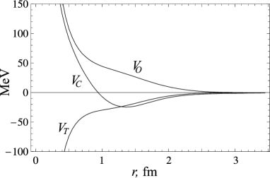
Figure 1: Exactly solvable potential (central $V_{C}$, tensor $V_{T}$ and spin-orbit $V_{O}$ terms) with parameters $k_{1}=0.944$, $k_{2}=0.232$ fm^-1 and $\chi=1.22$ fm^-1 taken from [20].

Comparing our results with those shown in figure 13 of paper [18], one can see that in both cases the curves have the same shape. Note that the potentials (33), (34), as well as potentials constructed in [18], are singular at the origin and by this reason they differ essentially from potentials obtained by Newton and Fulton [19, 20]. We believe that the difference with Ref. [20] may be explained by a somewhat different input parameters. It is well-known that there is a family of potentials with the same scattering matrix, when there are bound states. In our case there is a single bound state and, hence, there could exist two additional parameters, $A_{d}$ and $A_{s}$, known as the asymptotic normalization constants which provide an iso-phase deformation of the potential with the given scattering matrix. The values of these free parameters are fixed in both our model and the approach of Kohlhoff-von Geramb by the following reason. Physically acceptable components of a matrix potential should not have long-range tails. By this reason, corresponding asymptotic normalization constants can be determined directly from the $S$-matrix residue at the bound state pole [22]. In particular, the ratio of the asymptotic normalization constants reads

$$\eta=\frac{A_{d}}{A_{s}}=\frac{{\rm res}S_{2,1}(k=ik_{2})}{{\rm res}S_{1,1}(k=ik_{2})}\,.$$

For the potential $V(r)$ (33), (34), as well as for the Kohlhoff-von Geramb potential, the parameter of $\eta$ is fixed by the value $\eta=k_{2}^{2}/(2\chi^{2})=0.018081$.

4 Conclusion

As it was pointed out by Andrianov et al [16], an essential feature of matrix Darboux transformations is that the coefficient before the derivative may be a singular matrix. We call such transformations singular transformations. Often these transformations allow one to find hidden symmetries of the problem [16]. Moreover, any one-channel transformation, being considered from a multichannel viewpoint, becomes singular. This leads to a problem of incorporating such transformations into a chain of conventional (i.e. regular) transformations.

For the resulting action of the chain of conventional matrix Darboux transformations, there exists a generalization [15] of the well known for the one-channel case Crum-Krein formulas [8, 9]. In the present paper, a method is developed which allows one to use one-channel and coupled-channel SUSY transformations on equal terms. We reformulated results obtained in [15] such that singular transformations of a special type are included into the chain as links of the same rights as the conventional (regular) transformations except that they should be realized before the regular transformations. This approach together with recently introduced eigenphase preserving transformations [14], may become an alternative to the Gelfand-Levitan-Marchenko method of solving the inverse scattering problem with the advantage that no needs exist for solving any integral equation. The values of the $S$-matrix poles are incorporated into the the potential as parameters.

We would like to emphasis that the use of exponential and spherical Bessel functions usually permits to fit the experimental scattering data with a very high precision. This means that both the potential and solutions of the corresponding Schrödinger equation are expressed via determinants (see theorems 1 and 2 above) containing elementary functions only. We believe that this is a big advantage as compared to the Gelfand-Levitan-Marchenko method. Moreover, in contrast to the usual scheme where one applies transformations step by step, our approach permits one to skip all intermediate calculations and obtain the final potential directly in terms of solutions of the initial Schrödinger equation, i.e. usually in terms of elementary functions.

As an illustration of the method, using a special six-pole representation of the $S$ matrix, we derived a determinant representation of the Kohlhoff-von Geramb [18] solution to the Marchenko equation.

A drawback of the method, that we see, is that no a general recipe is known for choosing transformation matrices in a way to produce an Hermitian potential. Yet, in any concrete calculation this is enough to chose transformation matrices such that any intermediate potential is Hermitian. This is possible since corresponding condition is known [17] but the general problem is waiting for its solution.

Appendix A

Here we formulate the Sylvester identity [21]. Consider a square matrix of dimension $p+q$, $p,q=1,2,\ldots$

$$A=\left(\begin{array}[]{cccccc}a_{1,1}&\ldots&a_{1,p}&a_{1,p+1}&\ldots&a_{1,p+q}\\ &\ldots&&&\ldots&\\ a_{p,1}&\ldots&a_{p,p}&a_{p,p+1}&\ldots&a_{p,p+q}\\ b_{1,1}&\ldots&b_{1,p}&b_{1,p+1}&\ldots&b_{1,p+q}\\ &\ldots&&&\ldots&\\ b_{q,1}&\ldots&b_{q,p}&b_{q,p+1}&\ldots&b_{q,p+q}\\ \end{array}\right).$$ (A.1)

Let $a$ be the submatrix of dimension $p\times p$ composed of the elements $a_{i,j}$, $i,j=1,\ldots,p$. If to the bottom of $a$ we add a line of elements $b_{k,1}$, …, $b_{k,p}$, to the right of $a$ we add a column of elements $a_{1,p+l}$, …, $a_{p,p+l}$ and the right bottom corner we fill with the element $b_{k,p+l}$, we obtain a square matrix $m_{j,l}$. One says that $m_{j,l}$ is obtained from $A$ by embordering the block $a$ with $k$th row and $(p+l)$th column. The determinant $|m_{j,l}|$ is called an embordering minor in the determinant $|A|$. Since $k$ and $l$ can take the values $k,l=1,\ldots,q$ one has $q\times q$ embordering minors from which one can construct the matrix $M=(m_{j,l})$. The Sylvester identity relates the determinants $|M|$, $|A|$ and $|a|$ as follows:

$$|M|=|a|^{q-1}\,|A|\,.$$ (A.2)

References

References

- [1] Sukumar C V 1985 Supersymmetric quantum mechanics and the inverse scattering method J. Phys. A: Math. Gen. 18 2937–2955.
- [2] Baye D 1987 Supersymmetry between deep and shallow nucleus-nucleus potentials Phys. Rev. Lett. 58 2738–2741.
- [3] Baye D 1987 Phase-equivalent potentials from supersymmetry J. Phys. A: Math. Gen. 20 5529–5540.
- [4] Ancarani L U and Baye D 1992 Iterative supersymmetric construction of phase-equivalent potentials Phys. Rev. A 46 206–216.
- [5] Baye D 1993 Phase-equivalent potentials for arbitrary modifications of the bound spectrum Phys. Rev. A 48 2040 -2047.
- [6] Baye D and Sparenberg J-M 2004 Inverse scattering with supersymmetric quantum mechanics J. Phys. A: Math. Gen. 37 10223 -10249.
- [7] Samsonov B F and Stancu F 2002 Phase equivalent chains of Darboux transformations in scattering theory Phys. Rev. C 66 034001 (12pp).
- [8] Crum M M 1955 Assotiated Sturm-Liouville sistems Quart. J. Math. 6 121–127.
- [9] Krein M G 1957 On a continual analogue of the Christoffel formula from the theory of orthogonal polynomials Dokl. Akad. Nauk SSSR 113 970–973.
- [10] Samsonov B F and Stancu Fl 2003 Phase shift effective range expansion from supersymmetric quantum mechanics Phys. Rev. C 67 054005 (6pp).
- [11] Pupasov A, Samsonov B F, Sparenberg J-M and Baye D 2011 Reconstructing the nucleon-nucleon potential by a new coupled channel inversion method preprint arXiv:1101.3691v2 (to be published in Phys. Rev. Lett.).
-
[12]
Gelfand I M and Levitan B M 1951 On the determination of a
differential equation from its spectral function
Dokl. Akad. Nauk SSSR 77 557–560
Gelfand I M and Levitan B M 1951 On the determination of a differential equation from its spectral function Izvest. Akad. Nauk. SSSR Math. Series 15 309–360. - [13] Marchenko V A 1955 On reconstruction of the potential energy from phases of the scattered waves Dokl. Akad. Nauk SSSR 104 695–698.
- [14] Pupasov A M, Samsonov B F, Sparenberg J-M and Baye D 2010 Eigenphase preserving two-channel SUSY transformations. J. Phys. A: Math. Theor. 43 155201 (15pp).
- [15] Samsonov B F and Pecheritsin A A 2004 Chains of Darboux transformations for the matrix Schrödinger equation J. Phys. A: Math. Theor. 37 239–250.
- [16] Andrianov A A, Cannata F, Ioffe M V and Nishnianidze D N 1997 Matrix Hamiltonians: SUSY approach to hidden symmetries J. Phys. A: Math. Gen. 30 5037–5050.
- [17] Samsonov B F, Sparenberg J-M and Baye D 2007 Supersymmetric transformations for coupled channels with threshold differences J. Phys. A: Math. Theor. 40 4225–4240.
- [18] Kohlhoff H and von Geramb H V 1994 Coupled channels Marchenko inversion for nucleon-nucleon potentials Lecture Notes in Physics, Quantum Inversion Theory and Applications 427 (Berlin: Springer) 314–341.
- [19] Fulton T and Newton R G 1956 Explicit non-central potentials and wave functions for given -matrices Nuovo Cimento 3 677–717.
- [20] Newton R G and Fulton T 1957 Phenomenological neutron-proton potentials Phys. Rev. 107 1103–1111.
- [21] Gantmacher F R 1966 Théorie des Matrices 1 (Paris: Dunod).
- [22] Stoks V G J, van Campen P C, Spit W and de Swart J J 1988 Determination of the residue at the deuteron pole in an phase-shift analysis Phys. Rev. Lett. 60 1932–1935.