Collision of Viscoelastic Spheres: Compact Expressions
for the Coefficient of Normal Restitution

Abstract

The coefficient of restitution of colliding viscoelastic spheres is analytically known as a complete series expansion in terms of the impact velocity where all (infinitely many) coefficients are known. While beeing analytically exact, this result is not suitable for applications in efficient event-driven Molecular Dynamics (eMD) or Monte Carlo (MC) simulations. Based on the analytic result, here we derive expressions for the coefficient of restitution which allow for an application in efficient eMD and MC simulations of granular Systems.

Introduction and description of the system. The collision of frictionless (smooth) viscoelastic spheres obeys Newton’s equation of motion,

$$m_{\text{eff}}\ddot{\xi}=F\left(\dot{\xi},\xi\right),$$ (1)

with the effective mass $m_{\text{eff}}\equiv m_{1}m_{2}/(m_{1}+m_{2})$ and the compression $\xi\equiv R_{1}+R_{2}-\left|\vec{r}_{1}-\vec{r}_{2}\right|$, where $\vec{r}_{1}$ and $\vec{r}_{2}$ are the time dependent positions of the spheres. $F(\dots)$ is the normal component of the vectorial interaction force $F=\vec{F}\cdot\hat{e}$ with the unit vector $\hat{e}=\left(\vec{r}_{1}-\vec{r}_{2}\right)/\left|\vec{r}_{1}-\vec{r}_{2}\right|$. For non-adhesive viscoelastic spheres it reads brilliantov1996

$$F=F^{\text{el}}+F^{\text{dis}}=\min\left(0,-\rho\xi^{3/2}-\frac{3}{2}A\rho\sqrt{\xi}\dot{\xi}\right)\,$$ (2)

with

$$\rho\equiv\frac{2Y\sqrt{R_{\text{eff}}}}{3(1-\nu^{2})}$$ (3)

and $Y$, $\nu$ and $R_{\text{eff}}$ stand for the Young modulus, the Poisson ratio and the effective radius $R_{\text{eff}}\equiv R_{1}R_{2}/(R_{1}+R_{2})$, respectively. The dissipative constant $A$ is a function of the elastic and viscous material parameters brilliantov1996 . The $\min(\dots)$ function assures that the force is always repulsive.

The elastic part in Eq. (2), $F^{\text{el}}$, is the Hertz contact force hertz1882 while its dissipative part, $F^{\text{dis}}$, was first motivated in kuwabara1987 and then rigorously derived in brilliantov1996 ; morgado1997 , where only the approach in brilliantov1996 lead to an analytic expression of the material parameter $A$.

While the knowledge of the interaction force, Eq. (2) is sufficient to perform Molecular Dynamics simulations (MD), the coefficient of restitution is needed to perform much more efficient event-driven MD and Direct Simulation Monte Carlo (DSMC) as well as for the Kinetic Theory. By disregarding the dynamics of the collision process and idealizing the collision as an instantaneous event, the coefficient of restitution relates the postcollisional normal velocity, $\dot{\xi}^{\prime}$, to the normal component of the (precollisional) impact velocity, $v$,

$$\varepsilon\equiv-\dot{\xi}^{\prime}/v\,.$$ (4)

In general, the coefficient of restitution is not a constant but depends on the details of the interaction force and the impact velocity. It can be obtained by integrating Eq. (1) with the initial conditions $\xi(0)=0$ and $\dot{\xi}(0)=v$, assuming that the spheres start contacting at $t=0$. The coefficient of restitution is then obtained from

$$\varepsilon=-\dot{\xi}(t_{c})/v\,,$$ (5)

where the duration of the collision, $t_{c}$, is determined by the condition

$$\ddot{\xi}(t_{c})=0\,\qquad t_{c}>0\,,$$ (6)

that is, the collision terminates at time $t_{c}$ when the interaction force vanishes.

Solving the set of equations (5,6) is a complicated problem which was solved rigorously in schwager2008 . The solution reads

$$\varepsilon=1+\sum_{k=0}^{\infty}h_{k}\left(\beta^{1/2}v^{1/10}\right)^{k}\equiv 1+\sum_{k=0}^{\infty}h_{k}v_{\ast}^{k},$$ (7)

where we define the shorthand $v_{*}$ and with

$$\beta=\frac{3}{2}A\left(\frac{\rho}{m_{\text{eff}}}\right)^{2/5}\,.$$ (8)

This solution is exact since all coefficients $h_{k}$ are analytically known (see schwager2008 ). It is, moreover, universal since all material and particle properties are covered by $\beta$, that is, the $h_{k}$ are pure numbers which are independent of the material and particle properties.

Albeit exact, there are two main problems with the solution, Eq. (7), which prohibit its application in efficient MD or DSMC simulations: First, it converges extremely slowly. To obtain $\varepsilon$ up to quadratic order in $v$ we need 20 terms of the series expansion. Second, wherever we truncate the series at some order $k_{c}$, Eq. (7) diverges to $\varepsilon\to\pm\infty$, depending on the sign of $h_{k}$.

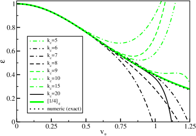
Figure 1: (color online) Coefficient of restitution, $\varepsilon$, over $v_{\ast}\equiv\beta^{1/2}v^{1/10}$. The analytic solution, Eq. (7), truncated at different order $k_{c}$ leads to divergence. The dotted line shows $\varepsilon$ as it follows from the numerical solution of Eqs. (5,6). It almost coincides with the thick green line showing the Padé approximant $[1/4]_{\varepsilon}$, Eq. (11), to the analytical solution, Eq. (7) (for explanation see the text below).

The divergence of the truncated series is a serious problem: Given the very accurate experimental data by Bridges et al. bridges1984 for the coefficient of restitution of ice balls at very low temperature whose material and particle properties correspond to $1.307\>(\text{sec/cm})^{1/5}$. From Fig. 1 we see that the series truncated at order $k_{c}=20$ starts deviating at $v_{*}\approx 1$ corresponding to the impact velocity $v=v_{*}^{10}/\beta^{5}\approx 0.262\>\text{cm/sec}$. That is, for typical impact velocities of $v\sim 1$ m/sec we would need to go to impractical high truncation order.

From an approximative expression for the coefficient of restitution for applications in efficient MD and DSMC simulations, we request that a) the approximative solution is close to the correct solution, b) it can be computed efficiently, that is, it contains only a small number of universal coefficients which are independent of the material and particle properties, and c) the representation must not reveal divergencies unlike the truncated series, Eq. (7), shown in Fig. 1.

Numerical solution. As described in schwager2008 ; ramirez1999 , Eq. (1) with the interaction force Eq. (2) and the corresponding initial conditions may be scaled to

$$\ddot{x}+x^{3/2}+v_{\ast}^{2}\,\dot{x}\sqrt{x}=0\,,\quad x(0)=0\,,\quad\dot{x}(0)=1$$ (9)

with the only free parameter $v_{*}\equiv\beta^{1/2}v^{1/10}$. Compression and time are scaled by $x\equiv\xi/[(\rho/m_{\text{eff}})^{-2/5}v^{4/5}]$ and $\tau\equiv t/[(\rho/m_{\text{eff}})^{-2/5}v^{-1/5}]$. From the numerical solution of Eq. (9) we determine $\varepsilon(v_{\ast})$ via Eq. (5): $\varepsilon=-\dot{\xi}(t_{c})/v=-\dot{x}(\tau_{c})$, where $\tau_{c}$ is obtained from the condition $\ddot{x}(\tau_{c})=0$, $\tau_{c}>0$. Apart from numerical errors, this solution is exact and may serve as a benchmark for our approximative solution, even for large values of $v_{\ast}$. Using the numerical solution we find the asymptotical behavior

$$\lim_{v_{\ast}\to\infty}\varepsilon(v_{\ast})=v_{\ast}^{-3.2}$$ (10)

for large $v_{\ast}$, in agreement with schwager2008 , see Fig. 2.

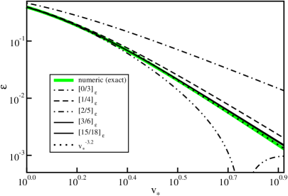
Figure 2: (color online) Coefficient of restitution $\varepsilon$ for large $v_{\ast}$. The thick green line shows the numerical solution of Eq. (9) revealing the asymptotic behavior $\varepsilon=v_{\ast}^{-3.2}$ (dotted line). Additionally various Padé approximants, Eq. (11), of the analytical solution, Eq. (7) are shown (discussion see text below). The Padé approximants $[3/6]_{\varepsilon}$ and $[15/18]_{\varepsilon}$ (virtually identical) agree almost perfectly with the exact solution.

Padé approximants. Using the analytical solution, Eq. (7), and the asymptotics, Eq. (10), we construct an approximative expression for $\varepsilon(v)$ which agrees with the analytical solution for the entire range of definition, $v\in(0,\infty)$, and is thus much more suitable for numerical simulations. The Padé approximant $[m/n]_{\varepsilon}(v_{*})$ approximates the $m+n$ times differentiable function $\varepsilon(v_{*})$ by a rational function

$$[m/n]_{\varepsilon}(v_{*})=\frac{\sum_{i=0}^{m}a_{i}v_{*}^{i}}{\sum_{i=0}^{n}b_{i}v_{*}^{i}}$$ (11)

in a way that the Maclaurin series of the approximant and of the approximated function match up to order $m+n$: $\varepsilon(0)=[m/n]_{\varepsilon}(0)$, $\varepsilon^{\prime}(0)=[m/n]_{\varepsilon}^{\prime}(0)$, …, $\varepsilon^{(m+n)}(0)=[m/n]_{\varepsilon}^{(m+n)}(0)$. Asymptotically, the Padé approximant behaves like a power law, $\lim_{v_{*}\to\infty}[m/n]_{\varepsilon}\sim v_{*}^{m-n}$. These properties allow to represent the function $\varepsilon(v_{*})$ similar to a Taylor expansion for small arguments and asymptotically as a power law, thus, convergent if $m<n$, see Ref. pade .

Since $\varepsilon\sim v_{*}^{\alpha}$ with $\alpha\approx-3$ (see Eq. (10) and Fig. 2) we chose a Padé approximation $[m/m+3]_{\varepsilon}$. To find an accurate yet compact approximant to Eq. (7) we start at $m=0$ and increase the order until sufficient agreement with the exact solution is achieved. The result is shown in Fig. 2: $[0/3]_{\varepsilon}$ is certainly not acceptable, $[1/4]_{\varepsilon}$ offers a good tradeoff between simplicity and accuracy. $[2/5]_{\varepsilon}$ reveals a pole at $v_{*}\approx 5.68$, therefore, it is suitable only for small impact velocity, $v_{*}\lesssim 10^{0.3}$. For ice spheres as described in bridges1984 this implies $v\lesssim 2.6\>\text{m/sec}$. The next order, $[3/6]_{\varepsilon}$, offers almost perfect agreement with the benchmark. We checked all orders up to $[25/28]_{\varepsilon}$ and could not find any significant improvement as compared to $[3/6]_{\varepsilon}$. As an example, $[15/18]_{\varepsilon}$ is shown in Fig. 2.

Table 1 displays the coefficients $a_{i}$ and $b_{i}$ for the relevant Padé approximants $[m/m+3]_{\varepsilon}$, $m\in\{0,1,2,3\}$ and

$m$	$n$	$a_{i}$	$b_{i}$
$0$	$3$	$a_{0}=1.$	$b_{0}=1$	$b_{2}=1.15345$
			$b_{1}=0$	$b_{3}=0$
$1$	$4$	$a_{0}=1.$	$b_{0}=1.$	$b_{3}=0.577977$
		$a_{1}=0.501086$	$b_{1}=0.501086$	$b_{4}=0.532178$
			$b_{2}=1.15345$
$2$	$5$	$a_{0}=1.$	$b_{0}=1.$	$b_{3}=0.638466$
		$a_{1}=0.553528$	$b_{1}=0.553528$	$b_{4}=0.384023$
		$a_{2}=-0.128445$	$b_{2}=1.025$	$b_{5}=0.027908$
$3$	$6$	$a_{0}=1.$	$b_{0}=1.$	$b_{4}=1.19449$
		$a_{1}=1.07232$	$b_{1}=1.07232$	$b_{5}=0.467273$
		$a_{2}=0.574198$	$b_{2}=1.72765$	$b_{6}=0.235585$
		$a_{3}=0.141552$	$b_{3}=1.37842$

Table 1: Coefficients of the Padé approximants $[m/m+3]_{\varepsilon}$ for $m\in\{0,1,2,3\}$. $[2/5]_{\varepsilon}$ reveals a pole at $v_{*}\approx 5.6801$.

Fig. 3 shows these Padé approximants together with the exact (numerical) solution. Again $[1/4]_{\varepsilon}$ and $[3/6]_{\varepsilon}$ turn out to be good compromizes between accuracy and simplicity.

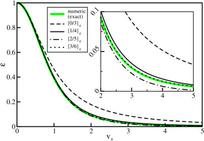
Figure 3: (color online) Coefficient of restitution $\varepsilon$ over $v_{\ast}$. The first four Padé approximants are shown together with the numerical (exact) solution. The inset shows a magnification. The order $[3/6]_{\varepsilon}$ (dotted line) coincides almost perfectly with the exact solution in the entire range of definition.

Conclusion. The universal exact solution, Eq. (7), for the coefficient of restitution of smooth viscoelastic spheres cannot be applied directly in eMD and DSMC simulations since the series diverges for any finite truncation order. We have shown that the Padé approximations of order $[1/4]_{\varepsilon}$ and $[3/6]_{\varepsilon}$ are suitable to represent the coefficient of restitution over the entire range of impact velocities including its asymptotic behavior up to an excellent accuracy and we provided the constants of this approximation. Similar as the full solution, Eq. (7), the Padé expansion is universal, that is, the constants $a_{i}$ and $b_{i}$ are universal. They neither depend on material properties (Young modulus, Poisson ratio, dissipative constant) nor on particle properties (radii, masses). All non-universal parameters enter exclusively via $\beta$, Eq. (8), which in turn enters the argument of the Padé expansion via $v_{*}=\beta^{1/2}v^{1/10}$ with $v$ being the impact velocity in physical units ($cm/sec$). Thus, the presented Padé approximation can be conveniently applied in numerical simulations.

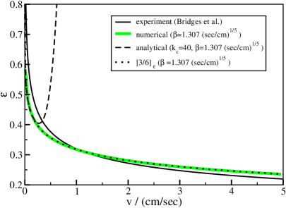
Figure 4: (color online) Coefficient of restitution $\varepsilon$ as a function of the impact velocity $v$. The Padé approximant $[3/6]_{\varepsilon}$ (dotted line) agrees almost perfectly with the numerical integration of Newton’s equation, Eqs. (1-6) in the entire range of impact velocity, $v$ (physical units), while the analytical solution, Eq. (7), truncated at order as large as $k_{c}=40$ diverges at $v\approx 0.3$ cm/sec. For the material constant, $1.307\>(\text{sec/cm})^{1/5}$, we used the experimental values by Bridges et al. bridges1984 for the collision of ice spheres at low temperature.

The precision of the approximant can be assessed in Fig. 4 which shows the Padé approximation together with the numerical integration of Newton’s equation, Eq. (1) in combination with Eqs. (2-6), and with the divergent analytical solution, Eq. (7), truncated at order as large as $k_{c}=40$. We see that over the entire range of definition, the Padé approximation coincides almost perfectly with the numerical solution and with the truncated analytical solution up to $v\approx 0.3$ cm/sec where it starts to diverge. For the material constant, $1.307\>(\text{sec/cm})^{1/5}$, we used the experimental values by Bridges et al. bridges1984 for the collision of ice spheres at low temperature. The corresponding data is also shown in the plot. While the agreement between the exact analytical result, the numerical integration and the Padé approximant is remarkable, the experimental data slightly deviates. This deviation is not surprising since besides viscoelasticity, described by the force Eq. (2), other forces may contribute, such as surface forces, plastic deformation, adhesion etc.

Acknowledgement. The authors gratefully acknowledge the support of the Cluster of Excellence ’Engineering of Advanced Materials’ at the University of Erlangen-Nuremberg, which is funded by the German Research Foundation (DFG) within the framework of its ’Excellence Initiative’.

References

- (1) N. V. Brilliantov, F. Spahn, J.-M. Hertzsch, and T. Pöschel, Phys. Rev. E 53, 5382 (May 1996)
- (2) H. Hertz, J. Reine Angew. Math 92, 156 (1882)
- (3) G. Kuwabara and K. Kono, Jpn. J. Appl. Phys. 26, 1230 (1987)
- (4) W. A. M. Morgado and I. Oppenheim, Phys. Rev. E 55, 1940 (Feb 1997)
- (5) T. Schwager and T. Pöschel, Phys. Rev. E 78, 051304 (2008)
- (6) F. G. Bridges, A. Hatzes, and D. N. C. Lin, Nature 309, 333 (May 1984)
- (7) R. Ramirez, T. Pöschel, N. V. Brilliantov, and T. Schwager, Phys. Rev. E 60, 4465 (1999)
- (8) G. A. Baker and P. Graves-Morris, Padé Approximants (Cambridge University Press, 1996)