Centrifugal force induced by relativistically rotating spheroids and cylinders

Abstract

Starting from the gravitational potential of a Newtonian spheroidal shell we discuss electrically charged rotating prolate spheroidal shells in the Maxwell theory. In particular we consider two confocal charged shells which rotate oppositely in such a way that there is no magnetic field outside the outer shell. In the Einstein theory we solve the Ernst equations in the region where the long prolate spheroids are almost cylindrical; in equatorial regions the exact Lewis ”rotating cylindrical” solution is so derived by a limiting procedure from a spatially bound system.

In the second part we analyze two cylindrical shells rotating in opposite directions in such a way that the static Levi-Civita metric is produced outside and no angular momentum flux escapes to infinity. The rotation of the local inertial frames in flat space inside the inner cylinder is thus exhibited without any approximation or interpretational difficulties within this model.

A test particle within the inner cylinder kept at rest with respect to axes that do not rotate as seen from infinity experiences a centrifugal force. Although the spacetime there is Minkowskian out to the inner cylinder nevertheless that space has been induced to rotate, so relative to the local inertial frame the particle is traversing a circular orbit.

PACS numbers 04.20.-q

1 Introduction

We aim to give a neat demonstration of centrifugal force on a static body which is induced by the rotation of a heavy shell that surrounds it. The shell causes the Minkowski space inside it to rotate, so, relative to that space, the static body moves backwards on a circle and experiences centrifugal force.

Pfister and Brown [9] have earlier studied this problem up to second order in $\Omega$ in a distorted sphere, however the problem can be more neatly solved to all orders using rotating cylinders. This was done by Embacher [3] generalizing work by Frehland [4]. Earlier papers on rotating cylindrical shells where by Papapetrou et al [10] and Jordan and McCrea [7].

The crucial property of cylinders is that centrifugal force-induced tensions retain the symmetry (unlike those in a sphere).

However the use of infinite rotating cylinders implies that space is not asymptotically flat and since the spacetime near the axis is Minkowskian there is some ambiguity in deciding which axes should be considered as non-rotating. We remove these difficulties by showing that the cylindrical equations are recovered as an approximation to the spaces inside and in between two tall prolate spheroidal shells which have no net angular momentum as they rotate in opposite senses about their axis. Outside both shells the space is static and tends asymptotically to flat Schwarzschild space at infinity. We demonstrate the strong analogy between rotating cylindrical shells in gravitation theory and solenoids in Maxwell’s electrodynamics . In the latter the magnetic flux that runs through a solenoid of finite length returns as a magnetic field outside it. As the solenoid is made longer and longer the flux returns over a wider and wider area, so, in the limit, as an infinite solenoid has a field strength of zero magnitude outside which nevertheless carries finite flux. This is the reason why there is no gravomagnetic field outside a rotating infinite cylinder. To ensure that all rotational effects are confined we shall treat two cylinders rotating in opposite directions so as to give no net angular momentum and no gravomagnetic flux outside the outer one.

2 Gravomagnetism and electromagnetism

There is a strong analogy between stationary electromagnetic fields and solutions of stationary metrics in General Relativity . Consider the stationary metric

$$ds^{2}=\xi^{2}(dt+A_{i}dx^{i})^{2}-\gamma_{ij}dx^{i}dx^{j}~{}~{}~{}i,j=1,2,3;~{}~{}~{}\xi=e^{-\psi}.$$ (2.1)

In the Newtonian limit $\psi$ is small and $\mbox{\boldmath$A$\unboldmath}~{}\!\!=0$. Even in strong field General Relativity Landau and Lifshitz’s equation may be rewritten, using 3-space metric’s $(\mbox{\boldmath$\nabla\!$\unboldmath}~{}\!\!\times\!\mbox{\boldmath$A$\unboldmath}~{}\!\!)^{j}=\eta^{jkl}\partial_{k}A_{l}$ where $\eta^{jkl}$ is the alternating symbol divided by $\sqrt{\det(\gamma_{ij})}$, in the form

$$\!\mbox{\boldmath$\nabla\!$\unboldmath}~{}\!\times\!(\xi^{3}\mbox{\boldmath$B\!$\unboldmath}~{})\!=2\kappa\mbox{\boldmath$J$\unboldmath}~{}~{}~{}~{},~{}~{}~{}\mbox{\boldmath$B\!$\unboldmath}~{}=(\mbox{\boldmath$\nabla\!$\unboldmath}~{}\!\times\!\mbox{\boldmath$A$\unboldmath}~{}\!\!)~{}~{}~{},~{}~{}~{}\kappa=\frac{8\pi G}{c^{4}}.$$ (2.2)

Here the divergensless current

$$J^{i}=\xi(T^{i}_{0}-{\textstyle{\frac{1}{2}~{}}\!}\delta^{i}_{0}T)=\frac{1}{\kappa}\xi R^{i}_{0}.$$ (2.3)

The above equations display the analogy to Maxwell’s with magnetic permeability $\xi^{-3}$. We shall therefore quote results of analogous electromagnetic problems to guide our understanding of solutions of Einstein’s equations.

In Newtonian gravitation a homoeoidal shell of mass $M$ on a prolate spheroid of semi-axes $a>b$ has the potential

$$\psi=m\textstyle{\ln\left(\sqrt{1+\frac{a^{2}}{\tilde{r}^{2}}}+\frac{a}{\tilde{r}}\right)}=\ln\left(\frac{\overline{r}+a}{\overline{r}-a}\right)^{m/2}\!\!~{},~{}r\geq b~{},~{}\psi=\textstyle{\frac{GM}{a}\ln\left(\sqrt{1+\frac{a^{2}}{b^{2}}}+\frac{a}{b}\right)}={\rm const}.~{},~{}r\leq b,$$

The last equation is Newton’s theorem; in (2),

$$m=\frac{GM}{a}~{}~{},~{}~{}R^{2}=\tilde{r}^{2}\sin^{2}\tilde{\theta}~{}~{},~{}~{}\tilde{r}^{2}=\overline{r}^{2}-a^{2},~{}~{}{\rm and}$$

$$dR^{2}+dz^{2}+R^{2}d\varphi^{2}=\frac{\overline{r}^{2}-a^{2}\cos^{2}\tilde{\theta}}{r^{2}-a^{2}}dr^{2}+R^{2}d\varphi^{2}+(\overline{r}^{2}-a^{2}\cos^{2}\tilde{\theta})d\tilde{\theta}^{2}.$$ (2.4)

Both $\tilde{r}$ and $\overline{r}$ are constant on prolate spheroids confocal with the shell. $\tilde{\theta}$ is constant on confocal hyperboloids and becomes the spherical polar $\theta$ at infinity. In the equatorial region $\tilde{r}=R+{\cal O}(z^{2}/a^{2})$. When $b<\tilde{r}\ll a$ the potential becomes that of a line of mass per unit length $M/(2a)=m/(2G)$, but at large $\tilde{r}$, $\psi\rightarrow GM/\tilde{r}$. The surface density of mass on the prolate spheroid is

$$\sigma=\frac{M}{4\pi ab\sqrt{\frac{b^{2}}{a^{2}}+\sin^{2}\tilde{\theta}}}.$$ (2.5)

A static charged prolate spheroidal conductor has an electrical potential of the form (2) but with the charge, $q$, replacing mass. If we now freeze the charge density (2.5) onto the spheroid by making it an insulator and rotate it about the axis with angular velocity $\Omega<c/b$, we find the magnetic field is uniform inside the shell and outside the magneto-static potential $\chi$ is given by

$$\chi=q\Omega\frac{b}{a}^{2}Q_{1}(\frac{\overline{r}}{a}),$$ (2.6)

$Q_{1}$ is the Legendre function of the second kind and $\overline{r}/a>1$.

We now consider two confocal prolate spheroids with positive charges $q_{1}$ and $q_{2}$. Each lies on an equipotential of the other so if they are both conductors their charge distributions is unaltered by the field of the other spheroid and then rotate the spheroids with angular velocities $\Omega_{1}>0$ and $\Omega_{2}<0$. The magnetic field is the sum of the fields of each, but as $\Omega_{2}<0$, they tend to cancel, except in the region between the spheroids . Externally the magnetic field potential is

$$\chi=\frac{1}{a^{2}}(q_{1}\Omega_{1}b_{1}^{2}+q_{2}\Omega_{2}b_{2}^{2})Q_{1}\!\!\left(\frac{\overline{r}}{a}\right)\cos\tilde{\theta}$$ (2.7)

which is zero if we chose

$$\Omega_{2}=-\frac{q_{1}b_{1}^{2}}{q_{2}b_{2}^{2}}\Omega_{1}.$$ (2.8)

The magnetic field inside both spheroids is of course uniform. We are interested in tall thin spheroids with $b_{1}<b_{2}\ll a$ and with the above choice the field inside both is

$$B_{I}=\frac{q_{1}\Omega_{1}}{a}\left(1-\frac{b_{1}^{2}}{b_{2}^{2}}\right)+{\cal O}\left(\frac{b^{2}}{a^{2}}\right)\!.$$ (2.9)

In this thin régime the field between the spheroids is approximately uniform in the equatorial region and carries equal and opposite flux to the field inside both so

$$B_{II}=-\frac{q_{1}\Omega_{1}b_{1}^{2}}{ab_{2}^{2}}.$$ (2.10)

The electrical potential outside both is given by (2) with $m=(q_{1}+q_{2})/a$.

3 Spheroidal shells in General Relativity 

We take the metrics in Weyl’s form for empty regions

$$ds^{2}=e^{-2\psi}(dt+A_{i}dx^{i})^{2}-e^{2\psi}\left[e^{2k}\left(dz^{2}+dR^{2}\right)+R^{2}d\varphi^{2}\right]\!.$$ (3.1)

where $k=0$ on the axis and $\mbox{\boldmath$A$\unboldmath}~{}\!\!=0$ when we deal with statics. The transformation from $z,R$ to $\overline{r},\tilde{\theta}$ coordinates is the same as in flat space considered earlier. Weyl showed that for axially symmetric statics Einstein’s equations imply $\nabla^{2}\psi=0$ where $\nabla^{2}$ is the flat space operator. The simplest spheroidal solution is the same as the classical one (2) and the corresponding metric function $e^{k}$ is

$$e^{k}=\left[1+\left(\frac{a}{\tilde{r}}\sin\tilde{\theta}\right)^{2}\right]^{-m^{2}/2}.$$ (3.2)

This metric can be generated by a single spheroidal shell the metric inside being flat. Babala [1] gives expressions for the stresses needed to support the shell against its own gravity. For prolate shells the energy conditions are most restrictive at the equator and the dominant energy condition is satisfied provided $|p_{\theta}|<\sigma$ there. From this we find that at fixed mass per unit length $m/2$, the dominant energy condition is always violated if the spheroidal shell is too tall so the cylindrical limit is not attainable. Nevertheless for quite relativistic $m$, axial ratios of order $100$ are attainable without violating the energy conditions so a cylindrical treatment is valid as an approximation in the equatorial region. For a spheroid of semi axes $\sqrt{a^{2}+b^{2}},b$, Babala’s condition [under his equation (12)] yields

$$m^{2}+(X^{2}-1)(1-Y)+\frac{1}{2}~{}X^{2}(1-Y^{-1})<mX,$$ (3.3)

where $X^{2}=1+b^{2}/a^{2}$ and $Y=[X^{2}/(X^{2}-1)]^{m^{2}/2}$. For large axial ratios, $X$ must be close to one and the above restriction on the axial ratio becomes

$$Y<\frac{1}{1-2m(1-m)},$$ (3.4)

corresponding to the restriction on the axial ratio

$$\alpha=\frac{\sqrt{a^{2}+b^{2}}}{b}<\frac{1}{[1-2m(1-m)]^{1/m^{2}}},$$ (3.5)

$\alpha$ is the axial ratio as measured in Weyl’s coordinates which exaggerate elongation. In the internal flat space its axial ratio is less by a factor $Y$ which is about $2$ for the three cases given below: For $m=1/3,\,Y<9/5,\,\,\alpha<198$, for $m=2/5,\,Y<25/13,\,\,\alpha<60$, and for $m=1/2,\,Y<2,\,\,\alpha<16$. Since parallel matter currents repel, these conditions will be slightly alleviated for a rotating spheroid.

When we have two oppositely rotating spheroidal shells we may choose the rotation of the outer shell to annul the angular momentum of the inner one. That ensures that there is no gravomagnetic moment of the whole system. Just as in electricity it is possible to choose rates within the outer shell so that there is no gravomagnetic field outside. The external field will then be static and predominantly of the form governed by equations (2), (2.7), (2.8) with $\mbox{\boldmath$A$\unboldmath}~{}=0$. However there may be some higher moment terms with

$$\psi=\psi_{0}+\sum_{n=1}^{\infty}a_{n}P_{n}(\tilde{\mu})Q_{n}\left(\frac{\overline{r}}{a}\right)$$ (3.6)

as given by Quevedo [11]. We are at liberty to choose the space within the inner shell to be flat space in rotating axes, i.e., with a uniform gravomagnetic field. For any chosen form of the inner shell $B_{n}$ and $\psi$ are continuous while discontinuities in $B_{||}$ and $\mbox{\boldmath$n\!\!$\unboldmath}~{}\!\cdot\!\mbox{\boldmath$\nabla\!$\unboldmath}~{}\psi$ give the matter currents and mass density on the shell. Between the shells the gravomagnetic field is in the $z$ direction on the equator by symmetry and will be close to that direction in the whole of the long straight region of tall spheroids. The Ernst equations in the empty region can be written in terms of flat space operators:

$$\mbox{\boldmath$\nabla\!$\unboldmath}~{}\!\!\cdot\!\!\left[e^{\psi}\mbox{\boldmath$\nabla\!$\unboldmath}~{}\!\!\left(e^{-4\psi}+\chi^{2}\right)\right]=0~{}~{}~{}{\rm and}~{}~{}~{}\mbox{\boldmath$\nabla\!$\unboldmath}~{}\!\!\cdot\!(e^{4\psi}\mbox{\boldmath$\nabla\!$\unboldmath}~{}\chi)=0,$$ (3.7)

and those imply

$$\nabla^{2}\psi={\textstyle{\frac{1}{2}~{}}\!}e^{4\psi}|\mbox{\boldmath$\nabla\!$\unboldmath}~{}\chi|^{2}.$$ (3.8)

In regions where the field is along the $z$ direction with $\chi=Hz$, the second of (3.7) is automatically satisfied if $\psi$ is a function of $R$ and the (3.8) may be written

$$Rd_{R}(Rd_{R}\psi)={\textstyle{\frac{1}{2}~{}}\!}H^{2}R^{2}e^{4\psi}$$ (3.9)

which equation is readily solved by writing $W=\psi+{\textstyle{\frac{1}{2}~{}}\!}\ln R$ and using $\ln R$ as the independent variable. We then recover the usual solution for rotating cylinders (see [7], [8], [14]):

$$e^{-2\psi}={\textstyle{\frac{1}{2}~{}}\!}HRC^{-1}\left[\left(\frac{R}{R_{0}}\right)^{-C}\!\!-\left(\frac{R}{R_{0}}\right)^{C}\right]\!,$$ (3.10)

where $C$ and $R_{0}$ are the constants of integration. For the region containing the axis $C=1$.

This derivation of the solution for rotating cylinders as a limiting case of thin prolate ellipsoids does not seem to be given before.

4 Metrics with oppositely rotating cylinders in General Relativity 

Consider two massive cylindrical shells rotating at constant angular velocity in opposite directions around a common axis of symmetry and surrounded on each side by empty space. The empty spacetime within the interior shell which we call shell one  or simply one  is flat. It is dragged around by the rotations of the shells. We therefore write its metric in cylindrical Minkowski coordinates rotating with constant angular velocity $\overline{\omega}$; say, $\{\overline{x}^{\mu}\}=\{\overline{x}^{0}=\overline{t},\,\overline{x}^{1}=\overline{R},\,\overline{x}^{2}=\overline{z},\,\overline{x}^{3}=\varphi\}$, then

$$d\overline{s}^{2}=\overline{g}_{\mu\nu}d\overline{x}^{\mu}d\overline{x}^{\nu}=(1-\overline{v}^{2})d\overline{t}^{2}+2\overline{R}\,\overline{v}d\overline{t}d\varphi-d\overline{R}^{2}-d\overline{z}^{2}-\overline{R}^{2}d\varphi^{2}~{}~{}~{}{\rm with}~{}~{}~{}\overline{v}={\overline{R}}{\overline{\omega}}~{}~{}{\rm for}~{}~{}{\overline{R}}\leq\overline{R}_{1}.$$ (4.1)

$\overline{R}_{1}$ denotes the position of one .

While within the inner cylinder spacetime is flat, seen from there the spacetime at infinity rotates at an angular speed $-\overline{\omega}$. Taking a global view we say that the flat spacetime within the inner cylinder rotates at a rate $\overline{\omega}$. A particle of rest mass $m_{0}$ which is forced to move in a circle at a rate $-\overline{\omega}$ with respect to the inner flat space has momentum

$$\mbox{\boldmath$\overline{p}$}=\frac{m_{0}\mbox{\boldmath$\overline{v}$}}{\sqrt{1-\overline{v}^{2}}}=-\frac{m_{0}\overline{v}}{\sqrt{1-\overline{v}^{2}}}\mbox{\boldmath$n$}_{\varphi}.$$ (4.2)

Its proper rate of change is

$$\frac{d\mbox{\boldmath$\overline{p}$}}{\sqrt{1-\overline{v}^{2}}d\overline{t}}=-\frac{m_{0}\overline{v}}{1-\overline{v}^{2}}\frac{d\mbox{\boldmath$n$}_{\varphi}}{d\overline{t}}=-\frac{m_{0}\overline{v}^{2}}{1-\overline{v}^{2}}\frac{\mbox{\boldmath$n$}_{R}}{\overline{R}}.$$ (4.3)

Thus the centrifugal force $F_{c}$ induced on a globally static particle is

$$F_{c}=\frac{m_{0}\overline{v}^{2}}{1-\overline{v}^{2}}\frac{1}{\overline{R}}.$$ (4.4)

Between one  and two  the metric is that of Lewis [8]. The metric in the form (3.1) offers some difficulties in finding physical values for the parameters of the second outer shell, i.e. one that satisfies the dominant energy conditions and does not rotate faster than the velocity of light. The following coordinates are more convenient. They resemble those of da Silva et al [12]. In coordinates $\{x^{\mu}\}=\{x^{0}=t,\,x^{1}=R,\,x^{2}=z,\,x^{3}=\varphi\}$, the metric, which contains 4 parameters, reads as follows:

$$ds^{2}=g_{\mu\nu}dx^{\mu}dx^{\nu}=fdt^{2}+2\frac{h}{\beta}dtd\varphi-R^{2(s^{2}-s)}(dR^{2}+dz^{2})-\frac{l}{\beta^{2}}d\varphi^{2}~{}~{}{\rm for}~{}~{}R_{1}\leq R\leq R_{2}.$$ (4.5)

In this,

$$f\!=\epsilon\,R\left(W-\frac{(\varpi+1)^{2}}{4W}\right),~{}h\!=\epsilon\,R\left(W-\frac{(\varpi^{2}-1)}{4W}\right),~{}l\!=\epsilon\,R\left(\frac{(\varpi-1)^{2}}{4W}-W\right)\!,$$

$$~{}~{}~{}~{}~{}~{}~{}~{}~{}~{}~{}~{}~{}~{}~{}~{}~{}~{}~{}~{}~{}~{}W\!=\!\alpha R^{2s-1}>0~{}~{}~{}{\rm and}~{}~{}~{}\epsilon=\pm 1.$$ (4.6)

The metric is invariant under linear transformations of $t,\varphi$ and can be transformed locally to the static Levi-Civita metric [13]. The parameter $\beta$ is introduced to normalize the angle $\varphi$ to vary from 0 to $2\pi$ in the whole of $\rm spacetime~{}\!\!$; vacuum cylindrical spacetimes with matter sources have in general conicities [2]. Without loss of generality we may assume $\beta>0$.

Outside shell two   spacetime is empty and static; the metric is that of Levi-Civita. In coordinates $\{X^{\mu}\}=\{X^{0}=T,\,X^{1}=\tilde{R},\,X^{2}=Z,\,X^{3}=\varphi\}$ the metric has the form (see, e.g., [14]):

$$d\tilde{s}^{2}=\tilde{g}_{\mu\nu}dX^{\mu}dX^{\nu}=\tilde{R}^{2m}dT^{2}-\tilde{R}^{2(m^{2}-m)}(d\tilde{R}^{2}+dZ^{2})-\frac{1}{\tilde{\beta}^{2}}\tilde{R}^{2(1-m)}d\varphi^{2}~{}~{}{\rm for}~{}~{}\tilde{R}\geq\tilde{R}_{2}.$$ (4.7)

The constant $\tilde{\beta}>0$ has a role similar to $\beta>0$ and $m$ is analogous to the parameter $m$ defined in (2.4).

Altogether there are 6 parameters involved in these metrics: $\alpha>0,\beta>0,\varpi,s,m$ and $\tilde{\beta}>0$ in addition to the “radii” of the shells $\overline{R}_{1},R_{1},R_{2}$ and $\tilde{R}_{2}$. $\alpha$ is a scale factor typical of spacetimes without an intrinsically defined scale. $\beta$ characterizes the conicity of spacetime between the two shells and $\tilde{\beta}$ the conicity of spacetime outside the outer shell. $s$ is associated with the mass of the inner shell. $\varpi$ is the parameter associated with the Coriolis force and the centrifugal force induced by the rotation of the cylinders. We shall refer to $\varpi$ as the parameter of induced centrifugal forces.

The metric on shell one   is obtained from (4.1) in which we set $\overline{R}=\overline{R}_{1}$ or from (4.5) by setting $R=R_{1}$:

$$ds_{1}^{2}=(1-\overline{v}_{1}^{2})d\overline{t}^{2}+2\overline{R}_{1}\,\overline{v}_{1}d\overline{t}d\varphi-d\overline{z}^{2}-\overline{R}_{1}^{2}d\varphi^{2}=f_{1}dt^{2}+2\frac{h_{1}}{\beta}dtd\varphi-R_{1}^{2(s^{2}-s)}dz^{2}-\frac{l_{1}}{\beta^{2}}d\varphi^{2}.$$ (4.8)

In this $f_{1},h_{1}$ and $l_{1}$ are the metric components (4.6) with

$$W~{}~{}~{}\rightarrow~{}~{}~{}W_{1}=\alpha R_{1}^{2s-1}.$$ (4.9)

$W_{1}$ is thus a measure of the distance of one   to the axis. The two metrics in (4.8) describe the same hypersurface. We must thus have:

$$\sqrt{1-\overline{v}_{1}^{2}}\overline{t}=\sqrt{f_{1}}t~{}~{}~{}{\rm and}~{}~{}~{}\overline{z}=R_{1}^{s^{2}-s}z,$$ (4.10)

up to constants of integration. We also need equality of the two remaining terms in the metric (4.8). This implies:

$$\overline{R}_{1}=\frac{1}{\beta}\sqrt{l_{1}}~{}~{}~{}{\rm and}~{}~{}~{}\overline{v}_{1}=\epsilon\left(W_{1}-\frac{\varpi^{2}-1}{4W_{1}}\right)\!,$$ (4.11)

$\overline{v}_{1}$ is the fastest “dragging velocity” of the flat interior.

The metric of two   is obtained from (4.5) in which we set $\tilde{R}=\tilde{R}_{2}$ or from (4.7) in which we set $R=R_{2}$:

$$ds_{2}^{2}=\tilde{R}_{2}^{2m}dT^{2}-\tilde{R}_{2}^{2(m^{2}-m)}dZ^{2}-\frac{1}{\tilde{\beta}^{2}}\tilde{R}_{2}^{2(1-m)}d\varphi^{2}=f_{2}dt^{2}+2\frac{h_{2}}{\beta}dtd\varphi-R_{2}^{2(s^{2}-s)}dz^{2}-\frac{l_{2}}{\beta^{2}}d\varphi^{2}.$$ (4.12)

The equality implies, among other things, that the term in $dtd\varphi$ is absent from $ds^{2}_{2}$, i.e.,

$$h_{2}=0~{}~{}~{}{\rm or}~{}~{}~{}W_{2}^{2}={\textstyle{\frac{1}{4}}}(\varpi^{2}-1)~{}~{};~{}~{}{\rm so}~{}~{}~{}f_{2}=-\epsilon\frac{R_{2}}{2W_{2}}(\varpi+1)~{}~{}~{},~{}~{}~{}l_{2}=-\epsilon\frac{R_{2}}{2W_{2}}(\varpi-1).$$ (4.13)

Other junction conditions will be dealt with below. Since $W^{2}_{2}>0$ we see that

$$\varpi^{2}>1~{}~{}~{}{\rm and}~{}~{}~{}\overline{v}_{1}=\epsilon\left(W_{1}-\frac{W_{2}^{2}}{W_{1}}\right).$$ (4.14)

The greatest dragging velocity $\overline{v}_{1}$ of the flat interior near one   depends essentially on the positions of the shells, for given $\alpha$ and $s$. The three other junction conditions, not yet mentioned, are similar to (4.10) and the first of (4.11):

$$\sqrt{f_{2}}t=\tilde{R}_{2}^{m}T~{}~{}~{},~{}~{}~{}R_{2}^{s^{2}-s}z=\tilde{R}_{2}^{m^{2}-m}Z~{}~{}~{}{\rm and}~{}~{}~{}\frac{1}{\beta}\sqrt{l_{2}}=\frac{1}{\tilde{\beta}}\tilde{R}_{2}^{1-m}.$$ (4.15)

A word about the conditions that spacetime between one   and two be locally Minkowski. These conditions are necessary and amount to ask that $g_{00}>0$ and $g_{33}<0$. If we add the condition that two   be outside of one , we have altogether three inequalities that must be satisfied:

$$f>0~{}~{}~{},~{}~{}~{}l>0~{}~{}~{},~{}~{}~{}{\rm and}~{}~{}~{}\frac{R_{2}}{R_{1}}>1.$$ (4.16)

This translates into the following conditions on the parameters. If

$$s>\frac{1}{2}~{}~{}, \varpi>1~{}~{},~{}~{}\epsilon=-1~{}~{}~{}{\rm and}~{}~{}~{}\textstyle{\frac{1}{4}}(\varpi-1)^{2}<W_{1}^{2}<W_{2}^{2}<\textstyle{\frac{1}{4}}(\varpi+1)^{2},$$ (4.17)

$${\rm or} \varpi<-1~{}~{},~{}~{}\epsilon=+1~{}~{}~{}{\rm and}~{}~{}~{}\textstyle{\frac{1}{4}}(\varpi+1)^{2}<W_{1}^{2}<W_{2}^{2}<\textstyle{\frac{1}{4}}(\varpi-1)^{2},$$ (4.18)

but if

$$s<\frac{1}{2}~{}~{}, \varpi>1~{}~{},~{}~{}\epsilon=-1~{}~{}~{}{\rm and}~{}~{}~{}\textstyle{\frac{1}{4}}(\varpi-1)^{2}<W_{2}^{2}<W_{1}^{2}<\textstyle{\frac{1}{4}}(\varpi+1)^{2},$$ (4.19)

$${\rm or} \varpi<-1~{}~{},~{}~{}\epsilon=+1~{}~{}~{}{\rm and}~{}~{}~{}\textstyle{\frac{1}{4}}(\varpi+1)^{2}<W_{2}^{2}<W_{1}^{2}<\textstyle{\frac{1}{4}}(\varpi-1)^{2}.$$ (4.20)

In either of these cases $\epsilon\varpi<0$ and one can easily check that the greatest dragging velocity never exceeds the speed of light:

$$-1<\overline{v}_{1}<1.$$ (4.21)

We now turn our attention to the structure of the shells.

5 Energy densities and pressures in the shells

The two shells have similar metrics (4.8) and (4.12). We write them collectively in the same form without indices 1 or 2:

$$d\sigma^{2}=\gamma_{ab}dx^{a}dx^{b}=fdt^{2}+2\frac{h}{\beta}dtd\varphi-R^{2(s^{2}-s)}dz^{2}-\frac{l}{\beta^{2}}d\varphi^{2}~{}~{}{\rm with}~{}~{}\{x^{a}\}=\{x^{0}=t,x^{2}=z,x^{3}=\varphi\}.$$ (5.1)

This is the metric of a hypersurface $R=$const in a spacetime whose metric $g_{\mu\nu}$ is given by (4.5). We assume the shells to be in the form of two-dimensional fluids rotating with angular velocity $\Omega$. The three velocity components $u^{a}$ are thus $u^{0},u^{2}=0,u^{3}=u^{0}\Omega$, with $u^{0}$ defined by the usual normalization $\gamma_{ab}u^{a}u^{b}=u_{a}u^{a}=1$. Let $\sigma$ be the mass-energy density, $p_{\varphi}$ the pressure or tension in the loops, and $p_{z}$ the vertical pressure or tension. The energy-momentum tensor of such a flow $\tau^{b}_{a}$ is necessarily of the following form in which all the components are constants:

$$\tau_{0}^{0}=(\sigma+p_{\varphi})u^{0}u_{0}-p_{\varphi}~{},~{}\tau^{0}_{3}=(\sigma+p_{\varphi})u^{0}u_{3}~{},~{}\tau_{3}^{3}=(\sigma+p_{\varphi})u^{3}u_{3}-p_{\varphi}~{}{\rm and}~{}\tau^{2}_{2}=-p_{z}.$$ (5.2)

There is also a $\tau^{3}_{0}$ component similar to $\tau^{0}_{3}$; other components are equal to zero. From these expressions and with $u_{a}u^{a}=1$ we may calculate the relevant physical quantities $\sigma,p_{\varphi},p_{z}$ and $\Omega$. Set

$$\Theta^{2}=(\tau^{0}_{0}-\tau^{3}_{3})^{2}+4\tau^{0}_{3}\tau^{3}_{0}.$$ (5.3)

Then,

$$\sigma={\textstyle{\frac{1}{2}~{}}\!}\![(\tau^{0}_{0}+\tau^{3}_{3})+\Theta]~{}~{},~{}~{}p_{\varphi}={\textstyle{\frac{1}{2}~{}}\!}\!\left[-(\tau^{0}_{0}+\tau^{3}_{3})+\Theta\right]~{}~{}~{},~{}~{}~{}p_{z}=-\tau^{2}_{2},$$ (5.4)

and

$$\Omega=\frac{d\varphi}{dt}=\frac{1}{2\tau^{0}_{3}}\left[-(\tau^{0}_{0}-\tau^{3}_{3})+\Theta\right]~{}~{}~{}\Rightarrow~{}~{}~{}v=\frac{\sqrt{l}}{\beta\sqrt{f}}\Omega,$$ (5.5)

$v$ is the proper velocity of the shell.

Next we can easily calculate the external curvature tensor components from both sides of the shell, say $K_{ab}$ and $\overline{K}_{ab}$. The surface energy-momentum tensor $\tau^{b}_{a}$ is given by

$$\tau^{b}_{a}=\frac{1}{\kappa}(\delta^{b}_{a}L^{c}_{c}-L^{b}_{a})~{}~{}~{}{\rm where}~{}~{}~{}L^{b}_{a}=K^{b}_{a}+\overline{K}^{b}_{a}~{}~{}~{}{\rm with}~{}~{}~{}\kappa=\frac{8\pi G}{c^{4}}.$$ (5.6)

If $n_{\mu}=g_{\mu\nu}n^{\nu}$ is the normal to the shell the expression of the external curvature components say $K_{ab}$ (and a similar expression for $\overline{K}_{ab}$) is as follows

$$K_{ab}=-\frac{\partial x^{\mu}}{\partial x^{a}}\frac{\partial x^{\nu}}{\partial x^{b}}D_{\mu}n_{\nu},$$ (5.7)

$D_{\mu}$ is a four covariant derivative in terms of the spacetime metric $g_{\mu\nu}$ (or $\overline{g}_{\mu\nu}$ or $\tilde{g}_{\mu\nu}$). For cylindrical shells and in the coordinates adopted, $K_{ab}$ is particularly simple to calculate:

$$K_{ab}=-{\textstyle{\frac{1}{2}~{}}\!}n^{1}\partial_{1}g_{ab}.$$ (5.8)

With the tensors $K^{b}_{a}$ and $\overline{K}^{b}_{a}$ we construct the tensors $L^{b}_{a}$ and $\overline{L}^{b}_{a}$ and with them the energy-momentum tensor of the shell given in (6.6).

So much about generalities.

6 Example of two shells of dust

In such shells there is no pressure in either direction $z$ or $\varphi$. If

$$p_{z}|_{1}=p_{z}|_{2}=0,$$ (6.1)

it follows from (5.2) and the evaluation of $\tau^{2}_{2}=0$, that

$$\frac{\beta}{\sqrt{l_{1}}}=\frac{1}{R_{1}^{\Sigma}}~{}~{}~{}{\rm and}~{}~{}~{}\frac{1}{\tilde{R}_{2}^{M}}=\frac{1}{R_{2}^{\Sigma}}.$$ (6.2)

The first equality determines $\beta$ and the second equality $\tilde{\beta}$ through $\frac{1}{\beta}\sqrt{l_{2}}=\frac{1}{\tilde{\beta}}\tilde{R}_{2}^{1-m}$, see (4.15). If in addition

$$p_{\varphi}|_{1}=p_{\varphi}|_{2}=0,$$ (6.3)

it follows from (5.4) and evaluating $\tau^{0}_{0},\tau^{3}_{3},\tau^{3}_{0}$ and $\tau^{0}_{3}$ that

$$p_{\varphi}|_{1}=0~{}~{}\Rightarrow~{}~{}\Theta|_{1}=\frac{1}{\kappa R_{1}^{\Sigma}}2s(1-s)~{}~{}~{}{\rm and}~{}~{}~{}p_{\varphi}|_{2}=0~{}~{}\Rightarrow~{}~{}\Theta|_{2}=\frac{1}{\kappa R_{2}^{\Sigma}}[2m(1-m)-2s(1-s)].$$ (6.4)

The energy per unit length and the velocities of the shells reduce thus to

$$\sigma|_{1}=\frac{1}{\kappa R_{1}^{\Sigma}}2s(1-s)~{}~{}~{},~{}~{}~{}v_{1}=\frac{\epsilon_{\varpi}}{|\varpi-1|}\Bigg{\{}\frac{\left[(\varpi-1)/2W_{1}\right]^{2}-1}{1-\left[(\varpi+1)/2W_{1}\right]^{2}}\Bigg{\}}^{1/2}\!\!\!\!\!\left[(2s-1)\varpi-1+2s(1-s)\right],$$ (6.5)

and

$$\sigma|_{2}=\frac{1}{\kappa R_{2}^{\Sigma}}[2m(1-m)-2s(1-s)],$$ (6.6)

$$v_{2}=-\frac{\epsilon_{\varpi}}{\sqrt{\varpi^{2}-1}}\left[(1-2s)\varpi+1-2m+2m(1-m)-2s(1-s)\right]\!.$$ (6.7)

The energy condition

$$\sigma|_{1}>0~{}~{}~{}{\rm amounts~{}to}~{}~{}~{}0<s<1,$$ (6.8)

but if we add the condition that $\sigma|_{2}>0$,

$${\rm then~{}~{}either}~{}~{}\frac{1}{2}~{}<s<1~{}~{},~{}~{}1-s<m<s~{}~{}~{}~{}~{}{\rm or}~{}~{}~{}~{}~{}0<s<\frac{1}{2}~{}~{}~{},~{}~{}s<m<1-s.$$ (6.9)

The parameters in these metrics and the associated physical quantities are intertwined in complicated ways. We can however see in (6.5) that $s$ characterizes the energy per unit length of the inner cylinder. $W_{1}$ for a given energy per unit length is a measure of the radius of the inner shell as we noticed before. We also noticed that $m$ represents the mass per unit length of spacetime far from the cylinders in the $R$ direction.

Equations (6.1) and (6.3) are 2 polynomials of order 2 in $\varpi(s)$ and $\varpi(s,m)$, see (6.4) and (6.6). There are thus twice 2 roots, say $\varpi_{\pm}(s)$ and $\varpi_{\pm}(s,m)$, which must be equal. This gives 4 possible solutions for $m(s)$ or $s(m)$. Mathematica solves such equations with great facility. It shows that among the four possible solutions only one satisfies the energy conditions in which

$$0<s<{\textstyle{\frac{1}{2}~{}}\!}~{}~{}~{}{\rm with}~{}~{}~{}s<m<1-s.$$ (6.10)

van Stockum [15] constructed in 1937 a rotating cylindrical shell of dust and showed that this is only possible if $s<{\textstyle{\frac{1}{2}~{}}\!}$.

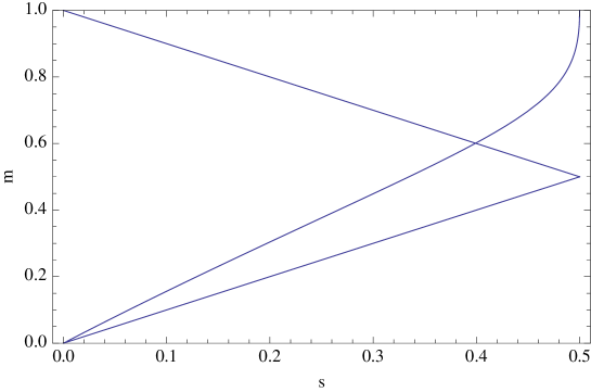
Figure 1: The function $m(s)$, implied by conditions (6.4), relates the total mass per unit length, $m$, to the parameter characterizing the mass per unit length of the inner shell, $s$. The straight lines are the limits $m=s$ and $m=1-s$ imposed by the energy condition on two . Above the triangle, the energy density of the outer shell is negative.

Figure 1 represents $m(s)$. From this figure we can see that the range of values which satisfy the energy conditions are in fact

$$0\leq s\ \lesssim 0.4~{}~{}~{}{\rm and}~{}~{}~{}0\leq m(s)\ \lesssim 0.6.$$ (6.11)

We also find that $\varpi<-1$ which implies, see (4.13), $\epsilon=1$ and, within the limits of $s$, that is

$$0\leq s\ \lesssim 0.4~{}~{}~{}\Rightarrow~{}~{}~{}-1.5\ \lesssim\varpi\leq-1.$$ (6.12)

Quantities analyzed so far depend on one parameter $s$ associated with the mass of the inner shell. However, the inner shell “radius”, or better $W_{1}=\alpha/R_{1}^{1-2s}$, is not fixed. According to (4.20):

$$W_{1min}=W_{2}=\sqrt{\frac{\varpi^{2}-1}{4}}<W_{1}<W_{1max}=\frac{1-\varpi}{2}.$$ (6.13)

It is useful to remember expression (4.3) from which follows that there is a smallest “radius” $R_{1min}$:

$$W_{1max}=\frac{\alpha}{R^{1-2s}_{1min}}.$$ (6.14)

When $W_{1}\rightarrow W_{1max}$ the following happens: Since $\varpi<-1$, $\epsilon=1$ and the proper radius of the inner shell tends to zero, see (4.11):

$$\overline{R}_{1}=\frac{1}{\beta}\sqrt{l}=\frac{1}{\beta}\left[R_{1}\left(\frac{W_{1max}^{2}}{W_{1}}-W_{1}\right)\right]^{1/2}~{}\rightarrow~{}0.$$ (6.15)

As $W_{1}$ approaches its (unattainable) maximal value $W_{1max}$, the metric component $g_{33}=-l/\beta^{2}\rightarrow 0$, the coordinate system becomes unphysical and the proper velocity of the inner shell, see (6.13), tends to zero:

$$v_{1}\propto\left[\frac{(W_{1max}/W_{1})^{2}-1}{1-[(\varpi+1)/2W_{1}]^{2}}\right]^{1/2}~{}\rightarrow~{}0.$$ (6.16)

The velocity of the inner shell as seen from the flat space inside approaches that of light and the angular velocity increases without bound as the radius $\overline{R}_{1}\rightarrow 0$. Calculating the dragging velocity from (4.11), we indeed find that it tends to the velocity of light:

$$\overline{v}_{1}=W_{1max}-\frac{W_{1min}^{2}}{W_{1max}}=1.$$ (6.17)

When, on the contrary, $W_{1}=W_{1min}=W_{2}$, we are dealing with two counter-rotating shells of dust with different energies per unit length and different velocities whose total angular momentum is equal to zero and there is no dragging inside.

For small mass-energies per unit length of the shells, i.e. in the Newtonian limit, $s\ll 1$, and for

$$m\simeq 1.618s~{}~{}~{},~{}~{}~{}\varpi\simeq-1-4s^{3}~{}~{}~{},~{}~{}~{}W_{2}\simeq\sqrt{2}s^{3/2}~{}~{}~{},~{}~{}~{}v_{2}\simeq-1.14s^{1/2},$$ (6.18)

and

$$\frac{W_{2}}{W_{1}}=\left(\frac{R_{1}}{R_{2}}\right)^{1-2s}\simeq\frac{R_{1}}{R_{2}},$$ (6.19)

we see from (6.5),

$$v_{1}\simeq s^{2}\left[\frac{1}{2s^{3}}\left(\frac{R_{1}}{R_{2}}\right)^{2}-2s^{3}\left(\frac{R_{2}}{R_{1}}\right)^{2}\right]^{1/2},$$ (6.20)

and,

$$\frac{|v_{2}|}{v_{1}}\simeq 1.618\left[\left(\frac{R_{1}}{R_{2}}\right)^{2}-4s^{6}\left(\frac{R_{2}}{R_{1}}\right)^{2}\right]^{-1/2}~{}~{}~{}{\rm with}~{}~{}~{}\sqrt{2}s^{3/2}\ \lesssim\frac{R_{1}}{R_{2}}\ \lesssim 1.$$ (6.21)

We thus see that to have strong dragging, in the classical limit, $|v_{2}|/v_{1}\simeq 1.618$, we need $R_{1}/R_{2}\thickapprox 1$. Otherwise, to have strong dragging we need $R_{1}/R_{2}\thickapprox s^{3/2}$. $R_{1}/R_{2}=0.1$ is already very relativistic.

It is interesting to have some idea of what the ratio of the velocities is in this relativistic case. Figure 2 shows the value of the maximum dragging velocity as a function of the parameter $s$.

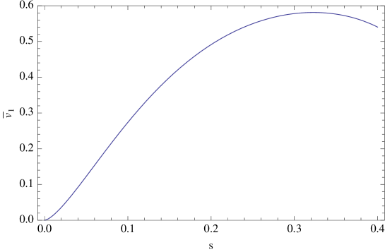
Figure 2: The dragging velocities $\overline{v}_{1}$ as functions of the parameter of the inner shell energy per unit length $s$ with $R_{1}/R_{2}=0.1$. At smaller ratios the maximum would still be higher.

We notice that the dragging $\overline{v}_{1}$ never exceeds $0.6$ and is only slightly greater than $(-v_{2})$ in the extreme relativistic case when $s\rightarrow 0.4$. In the Newtonian limit for small velocities,

$$\frac{\overline{v}_{1}}{(-v_{2})}\simeq 9.35v_{2}^{2}.$$ (6.22)

The velocity of the inner shell never exceeds $0.25$ and the ratio of velocities of the shells $v_{1}/(-v_{2})$ never exceeds $0.5$; in the Newtonian limit

$$\frac{v_{1}}{v_{2}}\simeq 0.124+0.256v_{2}^{2}.$$ (6.23)

Acknowledgments

J.B. and J.K acknowledge the hospitality of the Institute of Astronomy in Cambridge. J.B. acknowledges the hospitality of the Einstein Institute in Golm, the partial support from the Grant GAČR 202/09/00772 of the Czech Republic and the Grant No LC06014 and MSM0021620860 of the Ministry of Education.

References

[1]
Babala D 1986 Shell sources of stationary gravitational fields General Relativity and Gravitation18 173
[2] Bičák J, Ledvinka T, Schmidt B G and Žofka M 2004 Static fluid cylinders and their fields: global solutions Class. Quantum Grav.21 1583 (Preprint arXiv:gr-qc/0403012)
[3]
Embacher F 1983 Rotating hollow cylinders: General solution and Machian effects J. Math. Phys.24 1182
[4] Frehland E 1972 Exact gravitational field of the infinitely long rotating hollow cylinder Commun. Math. Phys.26 307
[5] Goldwirth D S and Katz J 1995 A comment on junction and energy conditions in thin shells Class. Quantum Grav.12 769 (Preprint arXiv:gr-qc/9408034)
[6] Israel W 1966 Singular hypersurfaces and thin shells Nuovo Cimento B44 1 and corrections in 1967 Nuovo Cimento B48 463
[7] Jordan S R and McCrea J D 1982 The gravitational field of a rotating infinite cylindrical shell J. Phys. A: Math. Gen15 1807
[8]
Lewis T 1932 Some special solutions of the equations of axially symmetric gravitational fields Proc. R. Soc. Lond. A136 176
[9]
Pfister H and Braun K H 1985 Induction of correct centrifugal force in a rotating mass shell Class. Quantum Grav.2 909
[10] Papapetrou A, Macedo A and Som M M 1978 Thin cylinder shell of dust under rigid rotation in General Relativity Int. J. Theor. Phys.17 975
[11] Quevedo 1989 General static axisymmetric solution of Einstein’s vacuum field equations in prolate spherical coordinates Phys. Rev. D39 2094
[12] da Silva M F A., Herrera L, Santos L O and Wang A Z 2002 Rotating cylindrical shell source for Lewis spacetime Class. Quantum Grav.19 3809 (Preprint arXiv:gr-qc/0206019)
[13] Stachel J 1982 Globally stationary but locally static space-times: A gravitational analog of the Aharonov-Bohm effect Phys. Rev. D26 1281
[14] Stephani H, Kramer D, MacCallum M, Hoenselaers C and Herlt E 2003 Exact solutions of Einstein’s field equations second edition (Cambridge: CUP) p.
342
[15] van Stockum W J 1937 The gravitational field of a distribution of particles rotating about an axis of symmetry Proc. R. Soc. Edinburg. A57 135