Solution for (1+1) dimensional surface solitons in thermal nonlinear media

Abstract

Analytical solutions for (1+1)D surface fundamental solitons in thermal nonlinear media are obtained. The stationary position and the critical power of surface solitons are obtained using this analytical solutions. The analytical solutions are verified by numerical simulations. The solutions for surface breathers and their breathing period, and solutions for surface dipole and tripole solitons are also given.

I introduction

In nonlinear optics, an optical beam forms a soliton when the self-focusing caused by the nonlinearity of the medium balances the diffraction. Recently, people pay more attention to nonlocal nonlinear media Snyder-1997-Science ; Krolikowski-2000-PRE ; Conti-2004-PRL ; Rotschild-2005-PRL . There are some types of solitons in nonlocal media, such as multipole-mode solitons Deng-2007-JOSAB ; Xu-2005-OL ; Rotschild-2006-OL , Laguerre and Hermite solitons Buccoliero-2007-PRL , and vortex solitons Rotschild-2005-PRL ; Alexander-2005-PRE ; Briedis-oe-2005 .

Surface waves have been studied generally in physics, chemistry and biology. They have been used to study the surface properties of media and the interaction between media and optical beams. In the presence of nonlinearity, some kinds of surface solitons have been found theoretically and experimentally, such as in local Kerr media Tomlinson-ol-1980 ; Mihalachea-pio-1989 , waveguide arrays Makris-ol-2005 ; Suntsov-prl-2006 ; Katashov-prl-2006 , photorefractive media Quirino-pra-1995 ; Cronin-Golomb-ol-1995 ; Aleshkevich-pre-2001 , and metamaterials Lazarides-pre-2008

Nowadays, surface solitons in nonlocal nonlinear media have been found theoretically and experimentally Alfassi-2007-PRL . An interesting property of surface solitons is that a beam launched away from the stationary position moves to the interface and oscillates at its vicinity, even if the launch position is far away from the stationary position. Now, varies types of surface solitons have been found and studied, such as incoherent surface solitons Alfassi-2009-PRA , surface dipoles Ye-2008-PRA ; V.Kartashov-2009-OL and surface vortices Ye-2008-PRA . Surface dipoles are found to be stable in the entire existence domain. Surface vortices are found to exhibit strongly asymmetric intensity and phase distributions. Bound states of surface vortex solitons belong to a class of surface solitons having no counterparts in bulk media Ye-2008-PRA .

However, there are no analytical solutions for the family of surface solitons due to the boundary conditions. We notice that the optical field of surface solitons almost resides in the nonlinear medium if the refractive index difference between two media is large enough. It is reasonable to assume that the optical intensity equals zero at the interface with large refractive index difference. In this paper, we obtain analytical solutions for the family of surface solitons and surface breathers under this assumption. Using the analytical solutions, we also obtain the stationary position and the critical power of surface solitons, and the breathing period of surface breathers. These results are proved by numerical simulations.

II surface fundamental solitons

First, we consider a (1+1)D sample sketched in Fig. 1(a) following the experiment in Ref. Alfassi-2007-PRL . The sample width $d$ is $1$ mm. The interface ($x=d$) between a nonlocal nonlinear medium (lead glass) with a refractive index $n_{1}=1.8$ and a linear medium (air) with a refractive index $n_{2}=1.0$ is thermally insulating, thus the temperature distribution $T$ satisfies the boundary condition $\partial T/\partial x|_{x=d}=0$. The other side of the sample is thermally conductive at the temperature $T_{0}$, $T_{0}$ is the temperature in the absence of light, thus the boundary condition is $T|_{x=0}=T_{0}$. The nonlinear refractive index change ($\Delta n$) of the sample satisfies the relation $\Delta n=\beta\Delta T=\beta(T-T_{0})$, where $\beta$ is the thermal coefficient of the refractive index. $\Delta n$ satisfies the conditions

$$\left.\frac{\partial(\Delta n)}{\partial x}\right|_{x=d}=0,\,\,\,\,\,\,\Delta n|_{x=0}=0.$$ (1)

$T$ satisfies the heat diffusion equation Rotschild-2005-PRL

$$\kappa\frac{\partial^{2}T}{\partial x^{2}}=-\alpha I,$$ (2)

where $\kappa$ is the thermal conductivity coefficient, $I$ is the optical intensity, $\alpha$ is the absorption coefficient.

We consider the propagation of a TE polarized laser beam along $z$ axis in the vicinity of the interface. In the nonlocal nonlinear medium ($0\leq x\leq d$), the slowly varying light field amplitude $U(x,z)$ (i.e. $I=|U|^{2}$) satisfies the nonlocal nonlinear Schrödinger equation,

$$2ik_{1}\frac{\partial U}{\partial z}+\frac{\partial^{2}U}{\partial x^{2}}+2k_{1}^{2}\left(\frac{\Delta n}{n_{1}}\right)U=0,$$ (3)

where $k_{1}=n_{1}k_{0}$, $k_{0}$ is wave number in vacuum and $|\Delta n|\ll n_{1}$. In the linear medium ($x\geq d$), $U(x,z)$ satisfies

$$2ik_{1}\frac{\partial U}{\partial z}+\frac{\partial^{2}U}{\partial x^{2}}+(k_{2}^{2}-k_{1}^{2})U=0,$$ (4)

where $k_{2}=n_{2}k_{0}$. Here we ignore the absorption of the medium, which is necessary for producing temperature changes and thermal nonlinearity. If the absorption is considered in propagation, the rigorous unchanged soliton does not exist in the nonlocal nonlinear medium due to the loss of the beam energy and the decreasing of the nonlinearity Huang-oc-2006 ; Cao-oc-2008 . Fortunately the propagation distances in most experiments are short enough so that the influence of the absorption can be ignorable Rotschild-2005-PRL ; Alfassi-2007-PRL ; Alfassi-2009-PRA . In order to show the stability of solitons in this paper, the propagation distances in numerical simulations are chosen to be 100-500 diffraction lengths, which are much longer than that in real experiments.

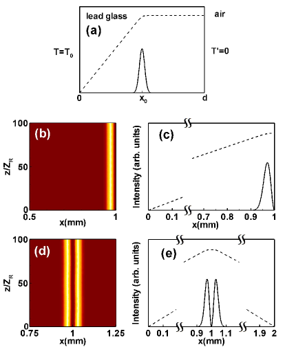
Figure 1: (Color online) (a) Sketch of a (1+1)D surface soliton. (b) Propagation of a surface soliton, and (c) its intensity and nonlinear refractive index profiles. (d) Propagation of a first-order Hermite-Gaussian soliton in a bulk medium, and (e) its intensity and nonlinear refractive index profiles. The beam width is $30$ $\mu$m and $Z_{R}=k_{1}w_{0}^{2}$ is the Rayleigh distance. The widths of the media are 1 mm for the surface soliton, and 2 mm for the bulk soliton, respectively. The solid line is the optical intensity profile and the dashed line is the nonlinear refractive index profile.

In Fig. 1(a), the solid line is the optical intensity profile for the beam launched at $x=x_{0}$ and the dashed line is the nonlinear refractive index which is not a bell shape. Obviously, the optical beam will approach to the interface where the nonlinear refractive index is larger, which presents the nonlinear attraction of the interface. The optical beam will be reflected when it arrives at the interface because the linear refractive index of the sample is larger than that of the air. When the nonlinear attraction balances the interface reflection, and simultaneously the nonlinear self-focusing balances the diffraction, the beam propagates stably along $z$ axis, which forms a surface soliton as shown in Figs. 1(b) and 1(c). Because the refractive index difference between two media is large enough, i.e. $n_{1}-n_{2}=0.8$, there is very little optical intensity residing in the air. In the simulation, the ratio of the optical intensity at the interface ($x=d$) to the maximum optical intensity is approximately $10^{-4}$, so the optical intensity at the interface can be negligible. Therefore we introduce the boundary conditions

$$I|_{x=0}=0,\,\,\,\,\,\,I|_{x=d}=0,$$ (5)

where $I|_{x=0}=0$ is valid because the optical beam is narrow and far away from the left boundary. Using above conditions and Eq. (1) for the temperature distribution, one can completely solve Eqs. (2) and (3) for the propagation of optical beams in the nonlinear medium, i.e. $0\leq x\leq d$. Here the physical influence of the linear medium, governed by Eq. (4) with continuous conditions at the interface, is simplified to the boundary condition $I|_{x=d}=0$ for the circumstance when the refractive index difference between two media is large enough.

To obtain analytical solutions for Eqs. (2) and (3), we consider a (1+1)D first-order Hermite-Gaussian (HG) soliton in a same bulk medium with the sample width $2d$, as shown in Figs. 1(d) and 1(e). The optical intensity satisfies the boundary conditions

$$I|_{x=0}=0,\,\,\,\,\,\,I|_{x=2d}=0,$$ (6)

because the optical beam is narrow and far away from the two boundaries. It also satisfies the condition

$$I|_{x=d}=0,$$ (7)

because the first-order HG function is antisymmetric and launched at the sample center ($x=d$). The temperature $T$ satisfies the conditions $T|_{x=0}=T_{0}$ and $T|_{x=2d}=T_{0}$, because the two boundaries of the sample are thermally conductive at the temperature $T_{0}$. Therefore the refractive index change satisfies the boundary conditions

$$\Delta n|_{x=0}=0,\,\,\,\,\,\,\Delta n|_{x=2d}=0.$$ (8)

The refractive index change is symmetrical for a symmetrical optical intensity, so it satisfies

$$\left.\frac{\partial(\Delta n)}{\partial x}\right|_{x=d}=0.$$ (9)

The evolution of the first-order HG soliton in the bulk medium ($0\leq x\leq 2d$) is governed by Eqs. (2) and (3) under the boundary conditions Eqs. (6) and (8). Comparing Eqs. (7) and (9) for the antisymmetric HG bulk soliton with Eqs. (1) and (5) for the surface soliton, one can find that the surface soliton is identical with the half part ($0\leq x\leq d$) of the first-order HG bulk soliton. Therefore, the solution of the surface soliton can be obtained from the solution of the first-order HG soliton in the bulk medium, namely,

$$U(x)=U_{0}H_{1}\left(\frac{x-d}{w_{0}}\right)\exp\left[-\frac{(x-d)^{2}}{2w^{2}_{0}}\right]\exp(-ibz),$$ (10)

where $H_{1}$ is the first-order Hermite polynomial, $w_{0}$ is the beam width, $b$ is the propagation constant, $U_{0}$ is a constant, and $0\leq x\leq d$.

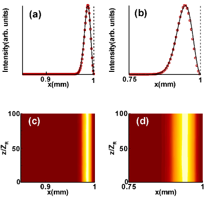
Figure 2: (Color online) The intensity profile of surface solitons for (a) $w_{0}=15$ $\mu$m and (b) $w_{0}=60$ $\mu$m. The square symbols represent the numerical solutions and the solid lines represent the analytical solutions. (c) and (d), propagations of surface solitons using the analytical solution as incident profile corresponding to (a) and (b), respectively. The sample width is 1 mm. The dashed lines indicate the interface.

Regarding the analytical solution as a trial solution, we will find the numerical soliton profile using the iterative method based on Eqs. (1)-(4). In our simulations, the parameters are $\alpha=0.01$ cm^-1, $T_{0}=25$ ^∘C, $\kappa=6.37\times 10^{-3}$ WK^-1cm^-1, $\beta=1.4\times 10^{-5}$ K^-1, $\lambda=514$ nm, which are the same as those in Ref. Alfassi-2007-PRL . The numerical profiles are calculated without the assumption $I|_{x=d}=0$, whereas all results of intensities at $x=d$ are small enough to be approximated to zero. Figs. 2(a) and 2(b) show the comparison of the optical intensity of the analytical solutions (solid lines) with the numerical solutions (square symbols) for $w_{0}=15$ $\mu$m [Fig. 2(a)] and $w_{0}=60$ $\mu$m [Fig. 2(b)]. One can see that the analytical solutions are in good agreement with the numerical solutions. Figs. 2(c) and 2(d) show the propagations of surface solitons using the analytical solutions Eq. (10) as incident profiles. The propagations are stable for a relative long distance, which verifies our analytical solutions again.

The critical power of surface solitons can be obtained from the analysis of bulk solitons. In the bulk medium, the nonlinear refractive index in Eq. (3) can be expanded at $x=d$, as Snyder-1997-Science

$$\Delta n=(\Delta n)^{0}-\frac{(x-d)^{2}}{2}\delta^{2}(P_{0}),$$ (11)

where $P_{0}$ is the input power of bulk solitons. The parameter $\delta^{2}$ can be found to be proportional to the beam intensity at $x=d$, or be proportional to $P_{0}/[\sqrt{\pi}w(z)]$, i.e.

$$\delta^{2}(P_{0})=\frac{\alpha\beta}{\kappa}\frac{P_{0}}{\sqrt{\pi}w(z)}.$$ (12)

Then, Eq. (3) reduces to a linear equation

$$2ik_{1}\frac{\partial U}{\partial z}+\frac{\partial^{2}U}{\partial x^{2}}-k_{1}^{2}\left(\frac{\alpha\beta}{n_{1}\kappa}\right)\frac{P_{0}}{\sqrt{\pi}w(z)}(x-d)^{2}U=0.$$ (13)

By substituting the solution of bulk solitons [same as Eq. (10) but $0\leq x\leq 2d$ ] into Eq. (13), and from the coefficient of each order term of $x$, we obtain the relation between the soliton power and the beam width in the bulk medium,

$$P_{c}=\frac{2\sqrt{\pi}n_{1}\kappa}{\alpha\beta k_{1}^{2}w_{0}^{3}}.$$ (14)

The critical power of surface solitons is half of that of bulk solitons, i.e. $P_{s}=P_{c}/2$. The amplitude constant $U_{0}=\sqrt{P_{c}}/(\sqrt{\pi}w_{0})^{1/2}$, and the propagation constant

$$b=\frac{3}{2k_{1}w_{0}^{2}}.$$ (15)

The stationary position $x_{s}$, namely the maximum optical intensity position of surface solitons, can be also obtained,

$$x_{s}=d-w_{0}.$$ (16)

Now the analytical solution for fundamental surface solitons is obtained completely. For example, in Fig. 2(c), the beam width $w_{0}$ is $15$ $\mu$m, the critical power $P_{s}$ is $888.4$ W/cm [in the simulation $P_{s}=892$ W/cm] and the stationary position is $15$ $\mu$m away from the interface. In Fig. 2(d), the beam width $w_{0}$ is $60$ $\mu$m, the critical power $P_{s}$ is $13.9$ W/cm [in the simulation $P_{s}=14.2$ W/cm] and the stationary position is $60$ $\mu$m away from the interface.

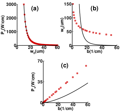
Figure 3: (Color online) (a) Relation between the critical power $P_{s}$ and the beam width $w_{0}$. (b) Relation between the beam width $w_{0}$ and the propagation constant $b$. (c) Relation between the soliton critical power $P_{s}$ and the propagation constant $b$. The solid line is the theoretical results and the square symbols are the numerical results.

Figure 3(a) shows the relation between the beam width and the critical power of surface solitons. The solid line is the theoretical value calculated by Eq. (14) and the square symbols are the numerical value. It can be seen that the theoretical value is in good agreement with the numerical value. The relation between the beam width and the propagation constant $b$ is shown in Fig. 3(b). One can see that there exists a great difference between the analytical solution and the numerical results. It means that Eq. (15) is incorrect because we neglect the higher order terms of the expansion of the nonlinear refractive index in Eq. (11). The higher order terms have little influence on the beam intensity and the critical power, but a great deal of influence on the phase change and the propagation constant. Because of the same reason, the dependence of the critical power $P_{s}$ on the propagation constant $b$ does not agree with the numerical solution, as shown in Fig. 3(c).

Figure 4: (a) The initial intensity distribution with $5\%$ noise. The intensity distributions of (b) after propagating $1$ Rayleigh distance and (c) after propagating $100$ Rayleigh distances. The beam width is $30$ $\mu$m.

In order to confirm the stability of our solutions, we simulate the beam propagation with perturbation based on Eqs. (1)-(4). The input condition is $U_{t}=U+\Delta U=U[1+\epsilon R(x)]$, where $\Delta U$ is the perturbation amplitude, $U_{t}$ is the total amplitude, $U$ is given by Eq. (10). $\epsilon$ is a perturbation constant, which is $5\%$ in our simulation. $R(x)$ is a random function whose value is between $0$ and $1$. Figure 4(a) shows the initial intensity distribution of the surface soliton with a great distortion. After propagating about $1$ Rayleigh distance as shown in Fig. 4(b), the distortion disappears and the intensity profile becomes smooth. Figure 4(c) shows the intensity distribution after propagating $100$ Rayleigh distances. This intensity distribution is still smooth and without distortion. Compared with Fig. 4(b), there is little change of the optical intensity profile in Fig. 4(c). So, the distorted profile can reform itself into a proper soliton after a short distance ($1$ Rayleigh distance) and propagate along the sample surface stably.

Figure 5: The sectional profile of the optical intensity of the surface soliton propagation for different sample widths. (a) The sample width $d=0.5$ mm $(\sim 16w_{0})$ , (b) $d=0.09$ mm $(3w_{0})$, and (c) $d=0.06$ mm $(2w_{0})$. The beam width is $30$ $\mu$m.

Finally, we discuss the influence of the sample width on the surface solitons. Fig. 1(b) shows the propagation of the surface soliton for the beam width $w_{0}=30$ $\mu$m and the sample width $d=1$ mm $(\sim 33w_{0})$, which is far greater than the beam width. If the sample width is reduced to $d=0.5$ mm $(\sim 16w_{0})$ as shown in Fig. 5(a), the propagation of the surface soliton is not influenced by the left boundary. And if the sample width is reduced to $d=0.09$ mm which is three times of the soliton beam width, the influence of the left boundary is still small. However when the sample width is reduced to $d=0.06$ mm $(2w_{0})$ as shown in Fig. 5(c), the propagation of the surface soliton is unstable and there is a great influence of the left boundary on the optical beam, and the optical beam can not form a stable soliton. We take the three times of beam width as a critical value. When $d/w_{0}=3$, the optical intensity at left boundary is about $I|_{x=0}/I_{max}\approx 3\times 10^{-3}$, and the influence of the left boundary is small enough to be negligible. When the sample width is smaller than three times of the beam width, $I|_{x=0}$ is not negligible, e.g. $I|_{x=0}/I_{max}\approx 0.1$ for $d/w_{0}=2$, and surface soliton can not exist due to the influence of the left boundary. This property is identical with that of solitons in bulk media Dong-2010-PRA .

III surface breathers

An optical beam can form a breather when the input beam power is stronger or weaker than the soliton critical power in the bulk medium. Fig. 6(b) ($P_{0}=2P_{c}$) and Fig. 6(d) ($P_{0}=P_{c}/2$) show the first-order HG breathers with $w_{0}=30$ $\mu$m in bulk media. Since the antisymmetry of the first-order HG beams in bulk media can retain during propagation, it is reasonable to expect that an optical beam launched at the sample surface also owns breathing effect. When the surface beam power is stronger than the soliton critical power, i.e. $P_{0}=2P_{s}$ as shown in Fig. 6(a), the optical beam approaches to the interface at first and converges because of the limit of the boundary. As the beam arrives at a position near the interface, it is reflected by the interface and diverges again. When the beam is far away from the interface, it is attracted again to the interface. This property is identical with the first-order HG breather in the bulk medium shown in Fig. 6(b) at $0\leq x\leq d$. If the surface beam power is weaker than the soliton power, i.e. $P_{0}=P_{s}/2$ as shown in Fig. 6(c), the breathing effect is opposite to the case of the stronger power. The optical beam is reflected by the interface and diverges at first, then attracted by the interface and returns back.

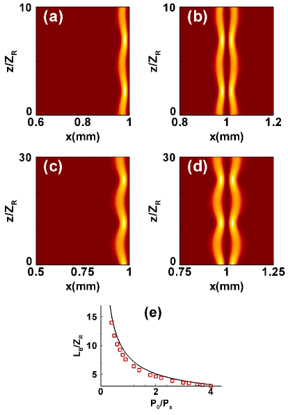
Figure 6: (Color online) The propagations of surface breathers and bulk breathers. (a)and (c), surface breathers with $P_{0}=2P_{s}$ and $P_{0}=0.5P_{s}$, respectively. (b)and (d), HG breathers with $P_{0}=2P_{c}$ and $P_{0}=0.5P_{c}$, respectively. The initial beam width is $w_{0}=30\mu m$ for all. (e) The relation between the surface breathing period and $P_{0}/P_{s}$ for the analytical value (solid line) and the numerical value (square symbols).

The analytical solution of surface breathers can be also obtained from the result of bulk breathers. In the bulk medium, we search for a breather solution for Eq. (3) in the HG function form

$$U(x)=U_{0}H_{1}\left[\frac{(x-d)}{w(z)}\right]\exp\left[-\frac{(x-d)^{2}}{2w(z)^{2}}+ic(z)(x-d)^{2}\right]e^{-ibz},$$ (17)

where $c(z)$ is the wavefront curvature. Substituting the breather solution into Eq. (13), and from the coefficient of each order term of $x$, we obtain two equations Guo-2004-PRE

$$\frac{dw(z)}{dz}-\frac{2c(z)w(z)}{k_{1}^{2}}=0,$$ (18a)

$$\frac{dc(z)}{dz}-\frac{1}{2k_{1}w(z)^{4}}+\frac{2c(z)^{2}}{k_{1}}+\frac{k_{1}}{2}\left(\frac{\alpha\beta}{n_{1}\kappa}\right)\frac{P_{0}}{2\sqrt{\pi}w(z)}=0.$$ (18b)

The combination of Eq. (18b) with the derivative form of Eq. (18a) yields

$$\frac{d^{2}[w(z)/w_{0}]}{d(z/Z_{R})^{2}}-\frac{1}{2[w(z)/w_{0}]^{3}}+\frac{P_{0}}{2P_{c}}=0,$$ (19)

Using the method introduced in Ref. Guo-2004-PRE , we obtain

$$w(z)=w_{0}\left[\sqrt{\Lambda}+\sqrt{\frac{5\Lambda(\Lambda-1)}{3}}\cos\left(\sqrt{\frac{3}{2}}\frac{z}{\Lambda Z_{R}}\right)\right],$$ (20)

where $\Lambda=(2P_{c}/P_{0})^{2/3}$. Then the parameters $c(z)$ and $b$ can be gotten and the solution of HG breathers in bulk media is obtained. The analytical solution of surface breathers is just the half part of Eq. (17), i.e. $0\leq x\leq d$. It should be noted that the critical power of surface breathers is a half of that of bulk solitons, i.e. $P_{s}=P_{c}/2$ .

From Eq. (20), the breathing period $L_{B}$ can be obtained as

$$L_{B}=\frac{2\sqrt{6}\pi Z_{R}}{3}\left(\frac{2P_{c}}{P_{0}}\right)^{2/3}.$$ (21)

A surface breather has a same period as its bulk counterpart. In Fig. 6(e), the analytical relation (solid line) approximates well to the numerical results (square symbols).

IV surface multipole solitons

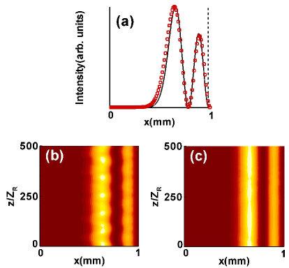
Figure 7: (Color online) (a) The profile of a dipole surface soliton. The square symbols are the numerical solution and the solid line is the analytical solution. (b) Propagation of the dipole soliton using the analytical solution as the incident profile. (c)Propagation of the dipole soliton using the numerical solution as the incident profile. The sample width is $1$ mm and the beam width is 250 $\mu$m.

In this section, we discuss the surface multipole solitons using the same method mentioned above. A surface dipole soliton can be expressed as a half part ($0\leq x\leq d$) of a third-order HG soliton in the center of a bulk medium ($0\leq x\leq 2d$). The profile of a dipole soliton (solid line) is shown in Fig. 7(a), and the numerical iterative solution (square symbols) is also shown for comparing. It can be seen that there exists a little difference between the numerical solution and the analytical solution. It is known that surface dipole solitons are stable V.Kartashov-2009-OL , analogously quadropole solitons in bulk media are stable too Dong-2010-PRA . The difference between the numerical solution and the approximate analytical solution can be considered as a perturbation, which leads to some spatial oscillations in propagation when the analytical solution is used as the initial profile, as shown in Fig. 7(b). However, the propagation using the numerical solution is stable as shown in Fig. 7(c).

A surface tripole soliton can be expressed as a half part ($0\leq x\leq d$) of a fifth-order HG soliton in the center of a bulk medium ($0\leq x\leq 2d$). The profile of a tripole soliton (solid line) is shown in Fig. 8(a), and the numerical iterative solution (square symbols) is also shown for comparing. There also exists a little difference between the numerical solution and the analytical solution. It has been proved in Ref. V.Kartashov-2009-OL that surface tripole solitons are unstable. As shown in Fig.8(c), the oscillation occurs after propagating over relatively long distance, i.e. $z/Z_{R}\approx 100$, when we use the numerical solution as the incident profile. When we use the approximate analytical solution, the perturbation resulted from the difference between the numerical solution and the approximate analytical solution grows up explosively. As a result, the strong oscillation takes place during the propagation as shown in Fig. 8(b). Anyway, our analytical solution coincides approximately with the numerical solution and it will be helpful for analyzing the multipole surface soliton propagation.

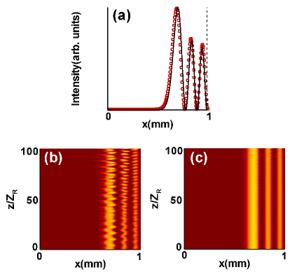
Figure 8: (Color online) (a) The profile of a tripole surface soliton. The square symbols are the numerical solution and the solid line is the analytical solution. (b) Propagation of the tripole soliton using the analytical solution as the incident profile. (c)Propagation of the tripole soliton using the numerical solution as the incident profile. The sample width is $1$ mm and the beam width is 120 $\mu$m.

V conclusion

In conclusion, the analytical solution for surface fundamental solitons has been found by comparing with bulk solitons, also for surface breathers, surface dipole and tripole solitons. The key assumption in this paper is that the optical fields all locate in the nonlinear medium when two media have large difference in the linear refractive index, and the intensity at the interface can be negligible as $I=0$. This method is similar to the image beam method Shou-2009-OL in dealing with the boundary force exerted on spatial solitons, which is an analogue of the well-known image charge method. By introducing image beams, the boundary conditions are automatically satisfied and analytical solutions can be found conveniently. The numerical simulations show our assumption is reasonable and correct. This method can be used also in dealing with other surface solitons if the linear refractive index difference between two media is large enough.

References

- (1) A. W. Snyder and D. J. Mitchell, Science 276, 1538 (1997).
- (2) W. Królikowski and O. Bang, Phys. Rev. E 63, 016610 (2000).
- (3) C. Conti, M. Peccianti, and G. Assanto, Phys. Rev. Lett. 92, 113902 (2004).
- (4) C. Rotschild, O. Cohen, O. Manela, M. Segev, and T. Carmon, Phys. Rev. Lett. 95, 213904 (2005).
- (5) D. Deng, X. Zhao, Q. Guo, and S. Lan, J. Opt. Soc. Am. B 24, 2537 (2007).
- (6) Z. Xu, Y. V. Kartashov, and L. Torner, Opt. Lett. 30, 3171 (2005).
- (7) C. Rotschild, M. Segev, Z. Xu, Y. V. Kartashov, L. Torner, O. Cohen, Opt. Lett. 31, 3312 (2006).
- (8) D. Buccoliero, A. S. Desyatnikov, W. Krolikowski, and Y. S. Kivshar, Phys. Rev. Lett. 98, 053901 (2007).
- (9) A. I. Yakimenko, Y. A. Zaliznyak, and Y. Kivshar, Phys. Rev. E 71 065603(R) (2005).
- (10) D. Briedis, D.E. Petersen, D. Edmundson, W. Krolikowski and O. Bang, Opt. Express, 13,435-443(2005).
- (11) W. J. Tomlinson, Opt. Lett. 5, 323-325 (1980).
- (12) D. Mihalachea, M. Bertolottib and C. Sibiliab, Prog. Opt. 27, 227-313(1989).
- (13) K. G. Makris, S. Suntsov, D. N. Christodoulides, G. I. Stegeman, A. Hache, Opt. Lett. 30, 2466-2468 (2005).
- (14) S. Suntsov, K. G. Makris, D. N. Christodoulides, G. I. Stegeman, A. Hache, R. Morandotti, H. Yang, G. Salamo, and M. Sorel, Phys. Rev. Lett. 96, 063901 (2006).
- (15) Y. V. Kartashov, V. A. Vysloukh, and L. Torner, Phys. Rev. Lett. 96, 073901 (2006).
- (16) G. S. Garcia Quirino, J. J. Sanchez-Mondragon, and S. Stepanov , Phys. Rev. A 51, 1571-1577 (1995).
- (17) M. Cronin-Golomb, Opt. Lett. 20, 2075-2077 (1995).
- (18) V. Aleshkevich, Y. Kartashov, A. Egorov, and V. Vysloukh, Phys. Rev. E 64, 056610 (2001).
- (19) N. Lazarides, G. P. Tsironis, and Y. S. Kivshar, Phys. Rev. E 77, 065601(R)(2008).
- (20) B. Alfassi, C. Rotschild, O. Manela, M. Segev, and D. N. Christodoulides, Phys. Rev. Lett. 98, 213901 (2007).
- (21) B. Alfassi, C. Rotschild, and M. Segev, Phys. Rev. A 80, 041808 (2009).
- (22) F. Ye, Y. V. Kartashov, and L. Torner, Phys. Rev. A 77, 033829 (2008).
- (23) Y. V. Kartashov, V. A. Vysloukh, and L. Torner, Opt. Lett. 34, 283 (2009).
- (24) Y. Huang, Q. Guo, and J. Cao, Opt. Commun. 261, 175-180(2006).
- (25) L. Cao, Y. Zhu, D. Lu, W. Hu, and Q. Guo, Opt. Commun. 281, 5004-5008(2008).
- (26) L. Dong, and F. Ye, Phys. Rev. A 81, 013815 (2010).
- (27) Q. Guo, B. Luo, F. Yi, S. Chi, and Y. Xie, Phys. Rev. E 69, 016602 (2004).
- (28) Q. Shou, Y. Liang, Q. Jiang, Y. Zheng, S. Lan, W. Hu and Q. Guo, Opt. Lett. 34, 3523 (2009).