Bilayer LDPC Convolutional Codes for Half-Duplex Relay Channels

Abstract

In this paper we present regular bilayer LDPC convolutional codes for half-duplex relay channels. For the binary erasure relay channel, we prove that the proposed code construction achieves the capacities for the source-relay link and the source-destination link provided that the channel conditions are known when designing the code. Meanwhile, this code enables the highest transmission rate with decode-and-forward relaying. In addition, its regular degree distributions can easily be computed from the channel parameters, which significantly simplifies the code optimization. Numerical results are provided for both binary erasure channels (BEC) and AWGN channels. In BECs, we can observe that the gaps between the decoding thresholds and the Shannon limits are impressively small. In AWGN channels, the bilayer LDPC convolutional code clearly outperforms its block code counterpart in terms of bit error rate.

I Introduction

The relay channel was introduced in 1971 when van der Meulen [1] proposed a channel model consisting of one source, one relay, and one destination. The relay aids the communication between the source and the destination so that increased robustness, higher transmission efficiency, and/or larger coverage range can be achieved. As smallest but fundamental unit of large network topologies, the relay channel has been extensively studied focusing on both theoretical and implementation aspects.

Decode-and-forward (DF) relaying is the most researched protocol for relay channels. In particular, the design of distributed channel codes has attracted considerable attention. The concept of distributed Turbo coding (DTC) was proposed in [2], which offered a new fashion of distributed code design. Low-density parity-check (LDPC) codes were considered for distributed coding for example in [3], [4] and [5]. Different approaches were presented to optimize LDPC codes for given channel conditions. For LDPC block codes, an irregular degree distribution needs to be derived to match a given channel. For a variety of channel conditions, extensive re-optimization is required. This leads to a high complexity for code adaptation and may not be feasible in practice.

In this paper we propose to use LDPC convolutional codes for distributed channel coding in relay networks. LDPC convolutional codes were first proposed in [6] as a time-varying periodic LDPC code variation. Then the idea was further developed in, e.g., [7], [8]. Recently, it has been proven analytically in [9] that the belief-propagation (BP) decoding threshold of an LDPC convolutional code achieves the optimal maximum a posteriori probability (MAP) threshold of the corresponding LDPC block code with the same variable and check degrees. This code in turn approaches the capacity as the node degrees increase. Furthermore, regular LDPC convolutional codes allow us to avoid complicated re-optimization of the degree distributions for varying channel conditions. Meanwhile, LDPC convolutional codes enable recursive encoding and sliding-window decoding [8], which dispels the concerns over complexity and delay. Motivated by the good properties of LDPC convolutional codes, we consider in this paper the design of bilayer LDPC convolutional codes for the relay channel. A similar code construction was proposed in [10] for the wiretap channel. A protograph-based bilayer code was proposed in [11] which applies the concept of bilayer-lengthened codes. In contrast to [11] we present bilayer expurgated codes [5] in this paper.

In the following, we will discuss the construction of bilayer LDPC convolutional codes for given relay channels. We will prove analytically that the proposed bilayer code is capable of achieving the highest rate with DF relaying in binary erasure channels (BEC). Moreover, the regularity of degree distributions significantly simplifies the code optimization. Numerical results are provided to verify the theoretical analysis.

II Preliminaries

In this section, firstly we introduce the transmission model we use throughout the paper. Then we briefly review the coding strategy which leads to the highest achievable rate [12] with DF relaying. The construction of bilayer codes [5] is described as a practical realization of the coding strategy.

II-A System Model

In this paper, we restrict ourself to the three-node relay channel which is composed of one source, one relay, and one destination. The source ($S$) intends to transmit its information to the destination ($D$) while the relay ($R$) provides assistance.

The system model is shown in Figure 1. Due to practical constraints the relay works in a half-duplex mode, which means it cannot transmit and receive at the same time or the same frequency. This implies that the transmission from the source to the destination is carried out in two phases. In the first phase, the source broadcasts while the relay and the destination listen. In the second phase, the relay transmits to the destination while the source keeps silent. We assume the transmissions on the three links to be orthogonal.

\psfrag{B}{\scriptsize${\boldsymbol{B}}$}\psfrag{D}{\scriptsize$\hat{{\boldsymbol{B}}}$}\psfrag{Xr}{\scriptsize${\boldsymbol{X}}\!_{R}$}\psfrag{Xs}{\scriptsize${\boldsymbol{X}}\!_{S}$}\psfrag{Y1}{\scriptsize${\boldsymbol{Y}}\!_{SR}$}\psfrag{Y2}{\scriptsize${\boldsymbol{Y}}\!_{SD}$}\psfrag{Y3}{\scriptsize${\boldsymbol{Y}}\!_{RD}$}\includegraphics[width=195.12767pt]{Fig/GerenalModel.eps}

Figure 1: Transmission model.

In the following we use $X_{i}$, $i\in\{S,R\}$, to denote the BPSK modulated signals which are transmitted from the source and the relay, and we use $Y_{i,j}$, $i\in\{S,R\}$, $j\in\{R,D\}$, for the channel observations of the three links. We use $C_{ij}=\emph{I}(X_{i};Y_{ij})$, $i\in\{S,R\}$, $j\in\{R,D\}$ to denote the capacity of each link constrained to the BPSK modulation. In this paper we assume that perfect channel-state information (CSI) is available for code construction.

II-B Achievable Rate

The highest transmission rate using decode-and-forward protocol for the half-duplex relay channel with orthogonal receive components is given as [12]

$$\begin{split}R_{DF}=\sup_{\alpha,0\leq\alpha\leq 1}\min(\alpha\emph{I}(X_{S};Y_{SR}&),\\ \alpha\emph{I}(X_{S};Y_{SD})+(1-&\alpha)\emph{I}(X_{R};Y_{RD}))\end{split}$$ (1)

where $\alpha$ is the fraction of channel uses in the first phase, and $(1-\alpha)$ is the fraction of channel uses in the second phase.

To achieve $R_{DF}$, in the first phase the source employs a capacity-achieving code for the source-relay link which guarantees successful decoding at the relay. This code may not be decodable at the destination due to the poorer channel condition on the source-destination link. Therefore, in the second phase the relay forwards additional bits to the destination in order to construct an overall lower rate code which is capacity-achieving for the source-destination link. A practical implementation of the idea is presented in the following.

II-C Bilayer LDPC Block Codes for Relay Channels

The construction of bilayer LDPC block codes [5] is realized in two steps corresponding to the two transmission phases.

In the first phase, $K_{1}$ information bits ${\boldsymbol{B}}$ are encoded by a length-$N_{1}$ codeword ${\boldsymbol{X}}_{S}$ through a rate-$R_{1}$ LDPC code $\mathcal{C}_{1}$ (i.e., $K_{1}=N_{1}\cdot R_{1}$) with the check matrix ${\boldsymbol{H}}_{S}$ and transmitted. At the end of the first phase, the relay decodes $\mathcal{C}_{1}$, using the check matrix ${\boldsymbol{H}}_{S}$, and recovers ${\boldsymbol{X}}_{S}$.

At the destination, additional $K_{2}$ bits are needed for successfully decoding ${\boldsymbol{X}}_{S}$:

$$K_{2}=N_{1}(\emph{I}(X_{S};Y_{SR})-\emph{I}(X_{S};Y_{SD})).$$

Therefore, in the second phase the relay generates $K_{2}$ new bits (syndrome, ${\boldsymbol{S}}$) using the check matrix ${\boldsymbol{H}}_{R}$. These $K_{2}$ syndrome bits are transmitted to the destination via a channel encoder $\mathcal{C}_{2}$ of rate $R_{2}$ using $N_{2}$ channel uses, i.e., $K_{2}=N_{2}\cdot R_{2}$. To simplify the discussion, we assume these syndrome bits are perfectly known at the destination after decoding $\mathcal{C}_{2}$. Then the overall code $\mathcal{C}$ is described by the stacked check matrix ${\boldsymbol{H}}$, and we have

$${\boldsymbol{H}}{\boldsymbol{X}}_{S}=\left[\begin{array}[]{c}{\boldsymbol{H}}_{S}\\ {\boldsymbol{H}}_{R}\end{array}\right]{\boldsymbol{X}}_{S}=\left[\begin{array}[]{c}{\boldsymbol{0}}\\ {\boldsymbol{S}}\end{array}\right].$$

That is, at the destination ($N_{1}-K_{1}$) zero check equations and $K_{2}$ non-zero check equations need to be satisfied in the decoding. The Tanner graph of a bilayer code example is plotted in Figure 2.

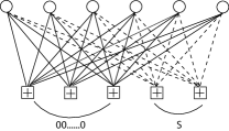
Figure 2: The Tanner graph of a bilayer LDPC code. Circles represent variable nodes, and squares indicate check nodes. The solid lines correspond to the edges in ${\boldsymbol{H}}_{S}$, and the dashed lines show the connections determined by ${\boldsymbol{H}}_{R}$.

To achieve the optimal performance, the design of ${\boldsymbol{H}}_{S}$ and ${\boldsymbol{H}}$ needs to guarantee that $\mathcal{C}_{1}$ and $\mathcal{C}$ are simultaneously capacity-achieving for the source-relay link and the source-destination link respectively. The authors of [5] approached this target by applying irregular LDPC block codes. Consequently, re-optimization is required for every given channel, which results in high complexity and infeasibility. In the next section we will show how this goal can be achieved by using regular LDPC convolutional codes leading to significantly reduced optimization overhead.

If the channel codes $\mathcal{C}_{1}$ and $\mathcal{C}_{2}$ are both capacity-achieving, i.e., $R_{1}=C_{SR}$ and $R_{2}=C_{RD}$, then the achievable rate in (1) is maximized by

$$\alpha=\frac{N_{1}}{N_{1}+N_{2}}=\frac{C_{RD}}{C_{RD}+C_{SR}-C_{SD}}.$$ (2)

Later in this paper we will prove that in BECs $R_{DF}$ can be achieved by applying bilayer LDPC convolutional codes.

III Bilayer LDPC Convolutional Codes

III-A LDPC Convolutional Codes

A regular $(l,r)$ time-varying binary LDPC convolutional code can be defined by a syndrome former matrix [8]

$${\boldsymbol{H}}^{T}=\left[\begin{array}[]{c c c c c}\ddots&&\ddots&&\\ {\boldsymbol{H}}_{0}^{T}(1)&\ldots&{\boldsymbol{H}}_{w}^{T}(1+w)&&\\ &\ddots&&\ddots&\\ &&{\boldsymbol{H}}_{0}^{T}(t)&\ldots&{\boldsymbol{H}}_{w}^{T}(t+w)\\ &&\ddots&&\ddots\\ \end{array}\right],$$

where $l$ is the variable degree and $r$ is the check degree. We assume that at each time instant $t$ ($t=1,2,...,L$) the number of variable nodes is $M$. Then each submatrix ${\boldsymbol{H}}_{i}^{T}(t+i)$ is a $M\times(Ml/r)$ binary matrix. The largest $i$ such that ${\boldsymbol{H}}_{i}^{T}(t+i)$ is nonzero for some $t$ is called the syndrome former memory $w$. The matrix ${\boldsymbol{H}}^{T}$ is sparse.

There are many variations of LDPC convolutional codes in the literature. In this paper, we denote an LDPC convolutional code by four parameters $\{l,r,L,w\}$. The memory constraint $w$ can be any non-negative integer. We assume that each of the $l$ edges of a variable node at time $t$ uniformly and independently connects to the check nodes in the time range $[t,...,t+w]$. More precisely, for each variable node at time $t$, one can define a type $\mathcal{M}_{t}$ [9] which is a $w$-tuple of non-negative integers, $\mathcal{M}_{t}=(m_{t,t},...,m_{t,t+j},...,m_{t,t+w})$, $j\in[0,w]$, and $\sum_{j}m_{t,t+j}=l$. The element $m_{t,t+j}$ indicates that there are $m_{t,t+j}$ edges connecting the designated variable node at time $t$ and the check nodes at time $t+j$. For each variable node, $\mathcal{M}_{t}$ is uniformly and independently chosen from all possible types. It has been stated in [9] that the $\{l,r,L,w\}$ code ensemble is capacity achieving and easier to analyze. However, experimentally it shows a worse trade-off between rate, threshold and block length.

Another variant, the $\{l,r,L\}$ ensemble, can be considered as a special case of the more general code ensemble mentioned above. For this ensemble, the memory length $w$ always equals $l-1$. Exactly one of the $l$ outgoing edges of each variable node at time $t$ is connected to one check node at position $[t,...,t+(l-1)]$, i.e., $m_{t,t+j}\!=\!1$ for all $j\in[0,l-1]$. We observe through experiments that this type of ensemble provides good performance with moderate $M$ and $L$ when $l\geq 3$.

In this paper, we use the $\{l,r,L,w\}$ ensemble for theoretical analysis while employing the $\{l,r,L\}$​ ensemble in simulations.

III-B Bilayer LDPC Convolutional Codes for Relay Channels

Firstly, we define the structure of a bilayer LDPC convolutional code. We assume the number of variable nodes to be $N=M\cdot L$. The connections between the $N$ variable nodes and the check nodes in the first (second) layer are determined by the ensemble $\{l_{1},r_{1},L,w_{1}\}$ ($\{l_{2},r_{2},L,w_{2}\}$). If $w_{1}=w_{2}$, we denote the bilayer code by $\{l_{1},l_{2},r_{1},r_{2},L,w\}$. Note that only the edges belonging to the same layer are connected to one check node. The structure of the overall check matrix is illustrated in Figure 3.

\psfrag{D}{${\boldsymbol{H}}^{T}$}\psfrag{A}{ ${\boldsymbol{H}}_{S}^{T}$}\psfrag{B}{${\boldsymbol{H}}_{R}^{T}$}\psfrag{E}{ $\ddots$}\includegraphics[width=151.76964pt]{Fig/BilayerMatrixT.eps}

Figure 3: Overall check matrix of a bilayer LDPC convolutional code. The white blocks correspond to the non-zero submatrices in the first layer, and the grey blocks are for those submatrices in the second layer.

The protocol for transmitting a bilayer LDPC convolutional code for the relay channel is similar to the strategy we explained in Section II-C. The information bits from the source are encoded by the single-layer code $\{l_{1},r_{1},L,w_{1}\}$ and broadcasted in the first phase. After successful decoding, the relay generates the syndrome bits using $\{l_{2},r_{2},L,w_{2}\}$. These syndrome bits are transmitted to the destination under perfect protection by another channel code in the second phase. The destination decodes the overall code by considering the zero check equations in the first layer and the non-zero check equations in the second layer.

III-C Analysis for Binary Erasure Channels

It has been shown in [9] that the $\{l,r,L,w\}$ ensemble with infinite $M$ has the following properties in a binary erasure channel: for the rate of the code $R$

$$\lim_{w\rightarrow\infty}\lim_{L\rightarrow\infty}R(l,r,L,w)=1-\frac{l}{r},$$ (3)

and for the decoding threshold

$$\lim_{w\rightarrow\infty}\!\lim_{L\rightarrow\infty}\!\epsilon^{B\!P}(l,r,L,w)\!=\!\!\lim_{L\rightarrow\infty}\!\epsilon^{M\!A\!P}(l,r,L,w)\!=\!\epsilon^{M\!A\!P}(l,r),$$

where $\epsilon^{BP}$ and $\epsilon^{MAP}$ are respectively the BP threshold and the MAP threshold for decoding. If we increase the degrees of the nodes, its decoding threshold approaches the Shannon limit $\epsilon_{Sh}=1-R$,

$$\lim_{r\rightarrow\infty}\lim_{w\rightarrow\infty}\lim_{L\rightarrow\infty}\epsilon^{BP}(l,r,L,w)=\epsilon_{Sh}.$$ (4)

In the following, we will show in Theorem 2 that the bilayer LDPC convolutional code $\{l_{1},l_{2},r,r,L,w\}$ achieves the same Shannon limit as the standard single-layer ensemble $\{l_{1}+l_{2},r,L,w\}$ [10]. As a preparation for the theorem, we introduce the following lemma.

Lemma 1.

If $M$, $L$ and $w$ go to infinity in this order, the density evolution of a single-layer LDPC convolutional code $\{l,r,L,w\}$ in a binary erasure channel can be written as

$$p^{(i)}=\epsilon(q^{(i-1)})^{l-1}\hskip 8.53581pt\mathrm{and}\hskip 8.53581ptq^{(i)}=1-(1-p^{(i)})^{r-1},$$

where $p^{(i)}$ ($q^{(i)}$) is the erasure probability from a variable (check) node to a check (variable) node in the $i$-th iteration, and $\epsilon$ is the erasure probability of the channel.

Proof.

In the following we refer to the check nodes connected to a given variable node as the active check nodes for that variable node. We use $p_{t,t+j}^{m,(i)}$ to denote the probability that the message from a given variable node at time $t$ to the $m$-th active check node at time $t+j$ in decoding iteration $i$ is erased. In the first iteration, $p_{t,t+j}^{m,(1)}=\epsilon$ for all $m$ and $j$. We use $q_{t+j,t}^{n,(i)}$ to represent the probability that the message from the $n$-th active check node at $t+j$ to the given variable node at $t$ is erased. Then we have

$$p_{t,t+j}^{m,(i)}=\epsilon\prod_{k=0,k\neq j}^{w}\left(\prod_{n=1}^{m_{t,t+k}}q_{t+k,t}^{n,(i-1)}\right)\cdot\prod_{v=1,v\neq m}^{m_{t,t+j}}q_{t+j,t}^{v,(i-1)}.$$ (5)

If $M\rightarrow\infty$, the messages from different nodes at the same time instant behave identically [8]. Then (5) reduces to

$$p_{t,t+j}^{(i)}=\epsilon\prod_{k=0,k\neq j}^{w}(q_{t+k,t}^{(i-1)})^{m_{t,t+k}}\cdot(q_{t+j,t}^{(i-1)})^{m_{t,t+j}-1}.$$ (6)

The messages from nodes at different time instants can behave differently and are usually tracked separately. However, if we have $L\rightarrow\infty$, the effect of boundaries caused by the initialization and the termination of the code vanishes. We can then consider the code asymptotically regular [13]. The message updating is averaged over $w+1$ time instants. Therefore, if $w\rightarrow\infty$, the messages from the nodes at different time instants have asymptotically identical distribution. Eventually, (6) is simplified to

$$p^{(i)}=\epsilon(q^{(i-1)})^{l-1}.$$

Similarly, we also obtain

$$q^{(i)}=1-(1-p^{(i)})^{r-1}.\vspace{-5mm}$$

∎

Now we look at the relation between the bilayer LDPC convolutional code ensemble $\{l_{1},l_{2},r,r,L,w\}$ and the standard single-layer ensemble $\{l_{1}+l_{2},r,L,w\}$.

Theorem 2.

[10] We denote a bilayer LDPC convolutional code of length $N=M\cdot L$ by $\{l_{1},l_{2},r_{1},r_{2},L,w\}$, where $l_{1}$ and $l_{2}$ are respectively the variable degrees of the two layers, $r_{1}$, $r_{2}$ are the check degrees of the two layers, and $w$ is the common memory constraint. If we assume the two layers take the same check degree, i.e., $r_{1}=r_{2}=r$, then the bilayer LDPC convolutional code $\{l_{1},l_{2},r,r,L,w\}$ approaches the same Shannon limit as the single-layer LDPC convolutional code $\{l_{1}+l_{2},r,L,w\}$.

Proof.

For the completeness of the proof, we repeat the derivation of the BP decoding threshold which was previously given in [10]. According to Lemma 1, we write for the first layer of the bilayer LDPC convolutional code,

$$p_{1}^{(i)}=\epsilon(q_{1}^{(i-1)})^{l_{1}-1}(q_{2}^{(i-1)})^{l_{2}}\hskip 5.69054pt\mathrm{and}\hskip 5.69054ptq_{1}^{(i)}=1-(1-p_{1}^{(i)})^{r_{1}-1}.$$

For the second layer of the code, we have

$$p_{2}^{(i)}=\epsilon(q_{1}^{(i-1)})^{l_{1}}(q_{2}^{(i-1)})^{l_{2}-1}\hskip 5.69054pt\mathrm{and}\hskip 5.69054ptq_{2}^{(i)}=1-(1-p_{2}^{(i)})^{r_{2}-1}.$$

Since $r_{1}=r_{2}=r$ and $p_{1}^{(1)}=p_{2}^{(1)}=\epsilon$, we obtain from the iterations $p_{1}^{(i)}=p_{2}^{(i)}$. Then the recursion can be written as

$$p^{(i)}=\epsilon(1-(1-p^{(i-1)})^{r-1})^{l_{1}+l_{2}-1}.$$

This indicates that the bilayer LDPC convolutional code has the same BP threshold as the $\{l_{1}+l_{2},r,L,w\}$ ensemble.

The rate of the bilayer LDPC convolutional code satisfies

$$\lim_{w\rightarrow\infty}\lim_{L\rightarrow\infty}R(l_{1},l_{2},r,r,L,w)=1-\frac{l_{1}}{r}-\frac{l_{2}}{r},\vspace{-1mm}$$ (7)

and the decoding threshold achieves the Shannon limit,

$$\lim_{r\rightarrow\infty}\lim_{w\rightarrow\infty}\lim_{L\rightarrow\infty}\epsilon^{BP}(l_{1},l_{2},r,r,L,w)=\frac{l_{1}}{r}+\frac{l_{2}}{r}.$$ (8)

According to (3) and (4), obviously the single-layer code $\{l_{1}+l_{2},r,L,w\}$ has the same rate as in (7) and achieves the same limit as in (8). Therefore, the theorem is proven. ∎

For the design of bilayer LDPC convolutional codes in relay channels, firstly we choose an $\{l_{1},r,L,w\}$ ensemble which is capacity achieving for the source-relay link. Afterwards the relay generates the syndrome bits according to $\{l_{2},r,L,w\}$ and forwards them to the destination. The overall code structure is consequently $\{l_{1},l_{2},r,r,L,w\}$. In the following we will show this overall code is capacity achieving for the source-destination link. In addition, it enables the highest achievable rate $R_{DF}$ of the relay channel.

Theorem 3.

For a binary erasure relay channel, we can find an LDPC convolutional code $\mathcal{C}_{1}=\{l_{1},r,L,w\}$ achieving the capacity for the source-relay link and simultaneously its bilayer extension $\mathcal{C}=\{l_{1},l_{2},r,r,L,w\}$ achieving the capacity for the source-destination link. Meanwhile, the above code construction provides the highest achievable rate with decode-and-forward relaying as in (1).

Proof.

We assume that the erasure probability for the source-relay link and the source-destination link are $\epsilon_{SR}$ and $\epsilon_{SD}$, respectively, and $\epsilon_{SR}<\epsilon_{SD}$. The corresponding channel capacities for these two links are

$$C_{SR}=1-\epsilon_{SR},\ C_{SD}=1-\epsilon_{SD}.$$

We use a regular LDPC convolutional code $\{l_{1},r,L,w\}$ with $l_{1}/r=\epsilon_{SR}$ for the transmission in the first phase. According to (3) and (4), we have

$$\lim_{w\rightarrow\infty}\lim_{L\rightarrow\infty}R(l_{1},r,L,w)=1-\frac{l_{1}}{r}=1-\epsilon_{SR}$$

$$\mathrm{and}\hskip 8.53581pt\lim_{r\rightarrow\infty}\lim_{w\rightarrow\infty}\lim_{L\rightarrow\infty}\epsilon^{BP}(l_{1},r,L,w)=\epsilon_{SR}.$$

Hence, $\mathcal{C}_{1}$ is capacity achieving, and error-free decoding can be guaranteed at the relay.

We assume that the number of variable nodes of $\mathcal{C}_{1}$ is $N_{V}$ and the number of check nodes of $\mathcal{C}_{1}$ is $N_{C1}$, then

$$N_{C1}=l_{1}N_{V}/r.$$

The number of additional bits needed at the destination is

$$N_{C2}=N_{V}(C_{SR}-C_{SD})=N_{V}(\epsilon_{SD}-\epsilon_{SR}),$$

and these bits are provided by the syndrome generated at the relay. At the destination, the total number of check nodes is

$$N_{C}=N_{C1}+N_{C2}=N_{V}(\frac{l_{1}}{r}+\epsilon_{SD}-\epsilon_{SR})=\epsilon_{SD}N_{V}.$$

The additional $N_{C2}$ check equations bring in $rN_{C2}$ edges, and the corresponding variable degree $l_{2}$ follows as

$$l_{2}=rN_{C2}/N_{V}=r(\epsilon_{SD}-\epsilon_{SR}).$$

From Theorem 2, we have for the source-destination link

$$\lim_{w\rightarrow\infty}\lim_{L\rightarrow\infty}R(l_{1},l_{2},r,r,L,w)=1-\frac{l_{1}+l_{2}}{r}=1-\epsilon_{SD},$$

$$\mathrm{and}\hskip 8.53581pt\lim_{r\rightarrow\infty}\lim_{w\rightarrow\infty}\lim_{L\rightarrow\infty}\epsilon^{BP}(l_{1},l_{2},r,r,L,w)=\epsilon_{SD}.$$

Therefore, the overall code $\mathcal{C}$ achieves the capacity of the source-destination link.

The number of channel uses in the first phase is $N_{1}=N_{V}$. In the second phase, we can use another capacity-achieving LDPC convolutional code to transmit the $N_{C2}$ syndrome bits to the destination. Therefore, $N_{2}=N_{C2}/C_{RD}$ channel uses are needed. The fraction

$$\alpha^{\prime}=\frac{N_{1}}{N_{1}+N_{2}}=\frac{C_{RD}}{C_{RD}+C_{SR}-C_{SD}}$$

equals the one in (2), which maximizes the achievable rate. ∎

From Theorem 3, we can conclude that the proposed regular bilayer LDPC convolutional codes significantly simplify the code optimization. Appropriate variable and check node degrees can easily be computed from the parameters of the channels, and a complicated optimization of irregular degree distributions as for example in [5] can be avoided.

IV Numerical Results

In this section, we firstly give numerical results for bilayer LDPC convolutional code ensembles $\{l,r,L\}$ in binary erasure relay channels. The source broadcasts its information bits with an $\{l_{1}\!\!=\!\!3,r\!\!=\!\!10,L\!\!=\!\!100\}$ LDPC convolutional code. At each time instant, the number of variable nodes is set to be $M\!=\!2000$. At the relay, different values of $l_{2}$ ($l_{2}\in\{2,3,4,5\}$) are chosen. Consequently, bilayer LDPC convolutional codes of different rates are constructed. Note that rate loss is inevitable for finite $L$ [8]. We compare the decoding thresholds of both the single-layer code and the bilayer codes with the corresponding Shannon limits. It can be seen from Figure 4 that the gaps in between are impressively small.

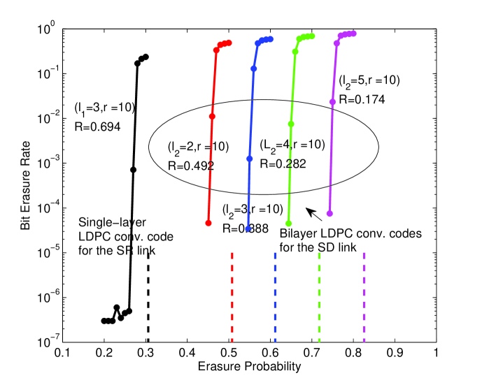
Figure 4: Bit erasure rate of bilayer LDPC convolutional codes with different overall rates in BECs. The solid curves show the simulation results, and the dashed lines indicate the Shannon limits.

To evaluate the proposed bilayer LDPC convolutional codes under more practical conditions, Figure 5 shows the bit-error-rate performance for the AWGN channel. For comparison purpose, we also include a regular bilayer LDPC block code. For both types of the codes, we set $l_{1}=3$, $l_{2}=2$, and $r=10$, which leads to approximately $R_{SR}=0.7$ and $R_{SD}=0.5$. In addition, the lengths of both codes are chosen in the way that the same hardware complexity [7] is needed. It can be observed that the bilayer LDPC convolutional code clearly outperforms its block code counterpart. Signal-to-noise ratio (SNR) gains of $0.5$ dB and $1.3$ dB are obtained at the relay and at the destination, respectively.

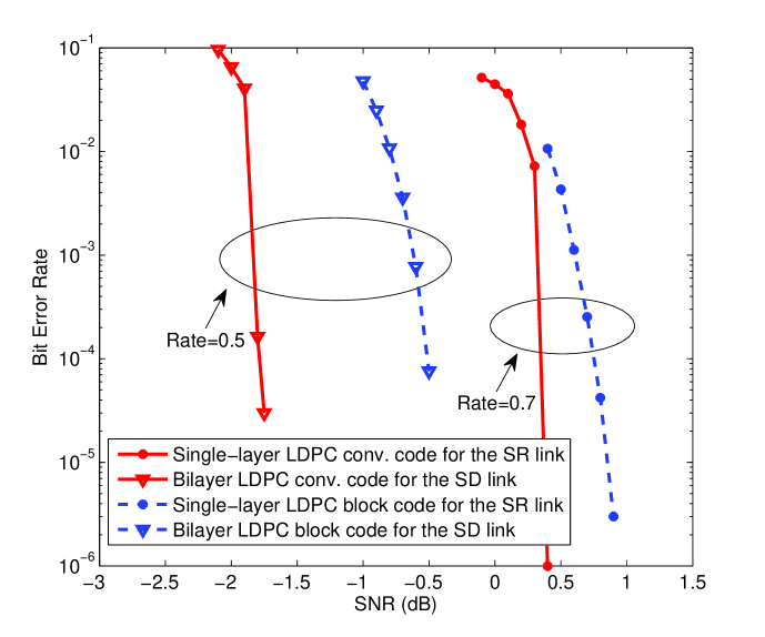
Figure 5: Comparison of bit error rate between a bilayer LDPC convolutional code and a regular bilayer LDPC block code in AWGN channels.

V Conclusions

In this paper bilayer LDPC convolutional codes were proposed for three-node relay channels. For a binary erasure relay channel, we can find a bilayer LDPC convolutional code which is able to simultaneously achieve the capacities of the source-relay link and the source-destination link. Meanwhile, this code provides the highest possible transmission rate with decode-and-forward relaying. Moreover, the regular code structure significantly reduces the complexity by avoiding the optimization of irregular degree distributions. Numerical results were provided in both binary erasure channels and AWGN channels. In binary erasure channels, we can observe that the decoding thresholds are very close to the Shannon limits. In AWGN channels, a significant gain in terms of SNR is achieved compared with its block code counterpart.

References

- [1] E. C. van der Meulen, “Three-terminal communication channels,” Advances in Applied Probability, vol. 3, pp. 120–154, 1971.
- [2] B. Zhao and M. C. Valenti, “Distributed Turbo coded diversity for relay channel,” Electron. Lett., vol. 39, no. 10, pp. 786–787, May 2003.
- [3] A. Chakrabarti, A. de Baynast, A. Sabharwal, and B. Aazhang, “Low density parity check codes for the relay channel,” IEEE Journal on Sel. Areas in Comm., vol. 25, no. 2, pp. 1–12, Feb. 2007.
- [4] J. Hu and T. M. Duman, “Low density parity check codes over wireless relay channels,” IEEE Trans. on Comm., vol. 6, no. 9, pp. 3384–3394, Sept. 2007.
- [5] P. Razaghi and W. Yu, “Bilayer low-density parity-check codes for decode-and-forward in relay channels,” IEEE Trans. on Inf. Theory, vol. 53, no. 10, pp. 3723–3739, Oct. 2007.
- [6] A. Jiménez Felström and K. Sh. Zigangirov, “Time-varying periodic convolutional codes with low-density parity-check matrix,” IEEE Trans. on Inf. Theory, vol. 45, no. 6, pp. 2181–2191, Sept. 1999.
- [7] A. E. Pusane, A. J. Felström, A. Sridharan, M. Lentmaier, K. Sh. Zigangirov, and D. J. Costello, “Implementation aspects of LDPC convolutional codes,” IEEE Trans. on Comm., vol. 56, no. 7, pp. 1060 – 1069, July 2008.
- [8] M. Lentmaier, A. Sridharan, D. J. Costello, and K. Sh. Zigangirov, “Iterative decoding threshold analysis for LDPC convolutional codes,” IEEE Trans. on Inf. Theory, vol. 56, no. 10, pp. 5274 – 5289, Oct. 2010.
- [9] S. Kudekar, T. Richardson, and R. Urbanke, “Threshold saturation via spatial coupling: Why convolutional LDPC ensembles perform so well over the BEC,” http://arxiv.org/abs/1001.1826v1, 2010.
- [10] V. Rathi, R. Urbanke, M. Andersson, and M. Skoglund, “Rate-equivocation optimal spatially coupled LDPC codes for the BEC wiretap channel,” http://arxiv.org/abs/1010.1669, 2010.
- [11] Thuy Van Nguyen, A. Nosratinia, and D. Divsalar, “Bilayer protograph codes for half-duplex relay channels,” in Proc. IEEE Int. Sympos. Information Theory (ISIT), 2010.
- [12] M. A. Khojastepour, A. Sabharwal, and B. Aazhang, “On capacity of Gaussian ’cheap’ relay channel,” in Proc. IEEE Global Telecommunications Conference (GLOBECOM), 2003.
- [13] M. Lentmaier, G. P. Fettweis, K. Sh. Zigangirov, and D. J. Costello, “Approaching capacity with asymptotically regular LDPC codes,” in Information Theory and Applications Workshop, Feb. 2009.