HORIZON: Accelerated General Relativistic Magnetohydrodynamics

Abstract

We present Horizon, a new graphics processing unit (GPU)-accelerated code to solve the equations of general relativistic magnetohydrodynamics in a given spacetime. We evaluate the code in several test cases, including magnetized Riemann problems and rapidly rotating neutron stars, and measure the performance benefits of the GPU acceleration in comparison to our CPU-based code Thor. We find substantial performance gains in comparison to a quad-core CPU both in single- and double-precision accuracy, and discuss these findings in the context of future numerical modeling efforts.

1 Introduction

Computational models of general relativistic flows are an important tool to understand the dynamics of compact objects, more so since gravitational wave detectors like LIGO, VIRGO, TAMA or GEO600 are becoming operational. To facilitate interpretation of data once they have been obtained, the inverse problem of determining source parameters can be studied with the help of simulated models.

General relativistic magnetohydrodynamics (GRMHD) is the study of magnetized flows under relativistic velocities and in very strong gravitational fields, and it is therefore ideally suited for modeling compact objects and their environments (for a review see Font (2008)). A number of GRMHD codes have been developed in recent years, see Koide et al. (1999), De Villiers & Hawley (2003), Gammie et al. (2003), Komissarov (2004), Antón et al. (2006), Mizuno et al. (2006), Anderson et al. (2006), Giacomazzo & Rezzolla (2007), Del Zanna et al. (2007), Yamamoto et al. (2008), Cerdá-Durán et al. (2008), Bucciantini & Del Zanna (2010) and Etienne et al. (2010). Most of these approaches employ finite-volume methods on structured meshes, and use high-resolution shock capturing schemes for handling the interface fluxes. Therefore, they are ideally suited for highly compressible flows with shocks, and enjoy conservative properties which also ensure numerical stability.

Since these models are computationally expensive, not least due to their proper account of ultrarelativistic motions and the general covariant form of the conservation laws, there is a strong impetus to explore the use of graphics processing units (GPUs) to accelerate the calculations. GPUs offer a substantially higher peak performance than traditional central processing units (CPUs) (Kirk & Hwu, 2010), and are better suited for the high throughput, data-parallel problems typical of large-scale simulations. Therefore, these architectures have become very popular in recent years, especially since vendors like NVIDIA have started to target the high-performance computing market with specific hardware features and appropriate software tools.

Graphics processing units have traditionally been designed for computer graphics algorithms. Most of these algorithms are data-parallel, i.e. the same operations are independently performed on a large stream of data. In contrast to central processing units, which are optimized for executing single threads rapidly, GPUs, as a data-parallel architecture, trade single-thread performance for massive parallelism. While CPUs perform computations on a few cores, current-generation GPUs may utilise hundreds or even over a thousand compute cores on a chip.

It is probably fair to say that GPUs do not only offer a much higher realizable performance at present, but also share architectural features which should become more prevalent in any hardware optimized for high throughput, data-parallel computations (Garland & Kirk, 2010). One reason is given by power and cooling considerations. Traditionally, commodity CPUs have gained speed by raising the frequency of operations, which gave rise to higher power consumption and more challenging cooling requirements. This approach cannot be scaled indefinitely, and therefore CPU designs have reached a power wall. A second factor is the memory wall: increasing latencies in accessing main memory are covered in CPUs by using large caches and sophisticated control logic, and the relative benefits of these approaches decrease with higher integration of the circuits.

GPUs use massive parallelism in place of large caches and expensive control logic, hiding memory access latencies with high-throughput computation on large streams (Garland & Kirk, 2010). Since more transistors are devoted to compute units compared to CPUs, the peak performance of GPUs (and similar architectures) is expected to increase substantially faster than in CPUs. Because of this, high-performance computing will greatly benefit from GPUs or similar designs in the future.

Attempts to use GPUs for scientific applications have increased rapidly with the recent introduction of NVIDIA’s CUDA language. Early adopters of this approach in astrophysics include Portegies Zwart et al. (2007), Belleman et al. (2008), Zink (2008), and Schive et al. (2008). Portegies Zwart et al. (2007), Belleman et al. (2008) and Schive et al. (2008) were concerned with N-body calculations (also using GRAPE, another parallel architecture), whereas Zink (2008) performed experiments on the general relativistic field equations. Barsdell et al. (2010) and Fluke et al. (2010) discuss future uses of GPUs in astrophysical simulations, and Choudhary et al. (2010) consider applications to numerical relativity. Herrmann et al. (2010) apply CUDA to the post-Newtonian equations describing the binary-black hole problem, and Khanna & McKennon (2010) investigate extreme-mass ratio inspirals. Specifically in the context of magnetohydrodynamics simulations, Pang et al. (2010) compare the performance of different hardware architectures. Wong et al. (2009), Wang (2009) and Wang et al. (2010) present implementations of (Newtonian) MHD in CUDA, and observe very promising performance relative to CPU implementations.

In this paper, we present an implementation of general relativistic magnetohydrodynamics on graphics processing units. The Horizon code is a standalone CUDA/C++ application which is in part based on the GRMHD code Thor (Zink et al., 2008; Korobkin et al., 2010). In the following, we will first briefly describe the physical system and the finite-volume method in section 2, and then present the Horizon code in section 3. In section 4, we evaluate the relative performance gain afforded by the GPU implementation compared to the CPU code. Afterwards, in section 5, we illuminate how differences between single and double precision arithmetics affect simulation results in a number of test cases. We conclude with a discussion in section 6.

2 Physical system and numerical method

2.1 Evolution system

The domain of Horizon are simulations of magnetized flows in general relativistic astrophysics. Similar to other codes in this field, e.g. Thor (Zink et al., 2008), WhiskyMHD (Giacomazzo & Rezzolla, 2007), CoCoNuT (Cerdá-Durán et al., 2008) and Sacra (Yamamoto et al., 2008), this allows to investigate the properties and dynamics of ultra-compact sources of gravitational radiation, including neutron stars, magnetars, and accretion flows around black holes.

In this paper we will only account for relativistic flows on a fixed spacetime background, which is known as the Cowling approximation in the context of stellar oscillations. Given such a spacetime metric $g_{\mu\nu}$, the conservation laws and Maxwell’s equations are (Font, 2008):

$$\nabla_{\mu}J^{\mu} = 0$$ (1)

$$\nabla_{\mu}T^{\mu\nu} = 0$$

$$\nabla_{\mu}F^{\mu\nu} = \mathcal{J}^{\nu}$$

$$\nabla_{\mu}{}^{*}F^{\mu\nu} = 0$$

Here, $J^{\mu}=\rho u^{\mu}$ is the rest-mass density current, $T^{\mu\nu}$ is the energy-momentum tensor of the fluid and the Maxwell field, $\mathcal{J}^{\nu}$ is the electric four-current, $F^{\mu\nu}$ is the Faraday tensor, and ${}^{*}F^{\mu\nu}$ is its Hodge dual.

We will assume the ideal MHD approximation to be valid in the following. Using a 3+1 split of Einstein’s field equations, and an associated decomposition of the GRMHD equations, we arrive at the conservation form (Noble et al., 2006)

$$\partial_{t}\left(\sqrt{-g}J^{t}\right)+\partial_{i}\left(\sqrt{-g}J^{i}\right)=0$$ (2)

$$\partial_{t}\left(\sqrt{-g}{T^{t}}_{\mu}\right)+\partial_{i}\left(\sqrt{-g}{T^{i}}_{\mu}\right)=\sqrt{-g}{T^{\kappa}}_{\lambda}{\Gamma^{\lambda}}_{\mu\kappa}$$

$$\partial_{t}\left(\sqrt{-g}B^{j}\right)+\partial_{i}\left[\sqrt{-g}(b^{i}u^{j}-b^{j}u^{i})\right]=0$$

$$\partial_{i}\left(\sqrt{-g}B^{i}\right)=0.$$

In these equations, we have used the magnetic field $B^{i}={}^{*}F^{it}$, the Christoffel symbols ${\Gamma^{\lambda}}_{\mu\kappa}$, and the magnetic four-vector $b^{\mu}$ is given in terms of the spacelike 3-hypersurface normal $n^{\mu}$ as $b^{\mu}=n_{\kappa}{}^{*}F^{\nu\kappa}({\delta^{\mu}}_{\nu}+u^{\mu}u_{\nu})/n_{\kappa}u^{\kappa}$. We identify the eight conservative quantities $\sqrt{-g}J^{t}$, $\sqrt{-g}{T^{t}}_{\mu}$ and $\sqrt{-g}B^{i}$ which form the basis of the finite-volume method.

Initial data for the evolutions reported later will be either given analytically (for Riemann problems) or will be imported from the publicly available rns code (Stergioulas & Friedman, 1995) for the construction of rapidly rotating neutron star models.

2.2 Overview of the numerical method

We discretize the system of conservation laws eqns. (2) with the use of a finite volume method and approximate Riemann fluxes at cell interfaces. This scheme has shock-capturing properties and is implemented in Thor and other GRMHD codes.

The system of conservation laws (2) can be written in the compact form

$$\partial_{t}w+\partial_{i}f^{i}(u(w))=s(u(w))$$ (3)

where $w$ is the tuple of conserved variables ($\sqrt{-g}J^{t}$ and so on), $u$ is the tuple of primitive variables ($\rho$ and so on), and $f^{i}$ is the flux vector. For the finite volume approach, we discretize the coordinate domain into a regular mesh of cells, and, for each cell, cast the conservation laws into a weak form by volume integration.

The evolution starts with converting the initial data, which is commonly given in terms of the primitive variables, into the conserved variables. The relation $w(u)$ is algebraic and can therefore be easily evaluated in each cell. For a time update, we need to evaluate the (time and area averaged) cell face flux vectors $f^{i}$. These are obtained from assuming a local Riemann problem at the center location of the face, and calculating the flux function appropriate for this problem.

The initial data for the face Riemann problems are obtained from the cell center data via a reconstruction. To avoid unphysical oscillations in the reconstructions these approximants are constrained by additional requirements (TVD and similar) which lead to extended reconstruction stencils compared to Lagrangian interpolants of the same order. Each cell interface needs data reconstructed at its left and right side to define the local Riemann problem.

After the initial state for the Riemann problem has been obtained, the appropriate flux is determined via a local operator on each face. Since the full Riemann problem is rather expensive to solve (and even more so when magnetic fields are included (Giacomazzo & Rezzolla, 2006)), we employ an approximate Riemann solver which only requires the values of the flux function from each (left and right) reconstructed primitive state, and the approximate maximal wave speeds associated with them.

When all face fluxes are known, we calculate the cell update from the effective flux per cell, and add the local source term contributions. We then have the new values of the conserved variables $w$, but to be able to continue with the next operation we will also need consistent primitive variables $u$. The inversion $u(w)$ is, unfortunately, not algebraic in general, so we employ a Newton-Raphson method to obtain the primitive state. This concludes a (sub-)step of the Runge-Kutta time advancement.

3 The Horizon code

3.1 Suitability of GPU architectures for general relativistic magnetohydrodynamics

Since the computational operations in the finite-volume model described above are local (inside the support of a small stencil of only a few cells), the problem is naturally data-parallel via domain decomposition. This fact has been used extensively in parallelizing GRMHD codes to distributed-memory architectures via MPI, such that each processor operates on a compact subset of the full domain, e.g. a block of $40^{3}$ cells. Boundary information is then shared via synchronization over ghost cells, and every time new data is needed for reconstruction, MPI messages are exchanged between (geometrically) adjacent processes. Then, each process operates independently on its block using local loops.

This type of coarse-grained block decomposition, while data-parallel, is not sufficient for using graphics processing units effectively. The number of processes in a typical MPI simulation will number in the tens or hundreds in many cases, whereas GPUs require tens or hundreds of thousands of threads to be saturated. The reason is that the simpler control logic and lower number of transistors devoted for advanced intermediate caches exhibit typically very high memory access latencies (in the order of several hundred cycles), which are hidden in the data parallel model by oversubscribing hundreds or thousands of compute cores with many more threads (see Garland & Kirk (2010) for details).

Therefore we will employ a fine-grained method of parallelism: here, each compute core on the GPU operates either on a single cell or a small set of cells. Given that a simulation may employ millions of cells in total, domain decomposition performed in this way can easily provide enough threads to saturate a GPU. If several GPUs are used for a larger simulation, a natural approach is to combine a coarse-grained decomposition into blocks as before, and then perform fine-grained parallel computation on each GPU.

Synchronization on the level of the GPU, which in itself is a shared-memory architecture, is easy to perform by executing independent compute kernels, and then using barrier statements to ensure that the global memory state on the device is consistent. Between GPUs, MPI synchronization using ghost cells can in principle be used as before, with the added complication that current MPI libraries cannot directly access the GPU memory, such that the transfer of ghost cells from the device memory to main memory (and back) must be performed before and after each MPI exchange.

Having addressed the matter of how to generate enough GPU threads and combine GPUs parallelism with MPI parallelism, a more challenging question concerns the kind of performance gains we can expect. Producing enough threads is easy in a naturally data-parallel problem of large size, but this is not the only important consideration as far as performance is concerned.

The reason many threads are employed is to hide main memory access latencies, as mentioned above. However, to achieve high performance the number of arithmetic (floating-point) operations in relation to main memory access operations, the so-called arithmetic intensity, must be high, so that the thread scheduler can run register-based operations in certain threads while other threads are still waiting for data. This can be a problem for simple operations like matrix-vector multiplication (extensively used e.g. in some elliptic solvers) and even simple Newtonian fluid dynamics codes, since the kernels then become limited by memory bandwidth, implying that processing cores are often idle waiting for data.

The theoretical memory bandwidth of a GPU is much higher than for a CPU, but it is only available if the programmer is very careful with data alignment and observes so-called coalescing rules while reading from memory. The latter refers to arranging memory operations within several threads in a particular way, such that load and store operations can be performed in a faster manner. Ignoring the (at times rather arcane) rules of memory access coalescence can significantly impact the available memory bandwidth (down to 1/10th in some architectures), and with it the available speedup for any application which is bandwidth-limited.

These coalescing rules are one of the main reasons GPU programming is known to be challenging. In the field of (Newtonian) computational fluid dynamics, which often has a low arithmetic intensity and, in addition, often needs to operate on unstructured meshes, efficient compute kernels are a major challenge for software developers. Some CFD methods, however, lend themselves to higher arithmetic intensities, e.g. Discontinuous Galerkin techniques, and are therefore considered for GPU applications (Klöckner et al., 2009).

Fortunately, this is precisely where GRMHD is different. The relativistic equations of motion contain many more operations per cell than is common for Newtonian finite-volume codes, even considering that more variables are needed to store the spacetime metric. The higher arithmetic intensity of GRMHD reduces the relative pressure on memory bandwidth from the compute kernels, and therefore can make use of a relatively larger portion of the (very high) compute performance of the GPU without excessive considerations of coalescing rules. The fact that recent architectures offer automatic caches makes the situation even more interesting for general-relativistic numerical codes.

There are additional performance considerations for writing fast GPU codes. Beside the memory coalescence, another important factor concerns the so-called block size. Current GPUs have a SIMD (single instruction multiple data) architecture also on the hardware level, in the sense that a number of compute cores are arranged into multiprocessors with a common instruction decoder. In practice, the GPU operates on a set of threads (a warp) in a single step, necessitating the exact same instruction to be performed up to the operands. The programmer can still use conditional statements for convenience (in contrast to explicit vector instructions), but if the command unit detects a divergence within a warp, the number of different code paths are serialized, with a comparable loss of available peak performance. For current architectures, this can be a factor of up to 32.

From the warp size, it is therefore desirable to have precisely common (essentially vectorized) execution parts at least as far as multiples of 32 are concerned. This is a concern with standard GRMHD in as far as the recovery of primitive variables are concerned, since the Newton-Raphson method may easily produce divergent execution paths depending on the cell data. However, in all experience from CPU simulations we do not expect this part of the code to be important for the overall speedup (even when considering Amdahl’s law (Amdahl, 1967)), and in addition the loss of performance from warp serialization competes with other possibly limiting factors. It is however important to arrange kernels to execute threads in a multiple of the warp size to use all cores effectively.

Another factor affecting performance also has to do with the way threads are distributed onto different multiprocessors. Each multiprocessor (remember that the GPU contains several such multiprocessors) contains fast local memory, which provides cache storage, but also space for the registers used for floating point operations. If several blocks of threads are assigned to a multiprocessor, they have to share the common memory resources. In adverse cases, this could lead to register spilling, where operands have to be “cached” into the device’s main memory, thereby strongly reducing available performance. Fortunately, it is possible to find a good thread configuration for each compute kernel simply by a set of small experiments.

Even the shared memory accesses can have varying performance since the memory is organized into banks, and random access to data can lead to bus conflicts and corresponding serialization. This, however, is often only a minor consideration when compared to other factors affecting performance, and recent architectural developments for GPUs have further decreased its relevance.

We have, so far, left out one of the likely most important influences on GPU performance in current architectures: the differences between single and double precision floating point operation cost. Historically, GPUs have evolved in the context of graphics applications, which typically do not require more than single-precision accuracy even in demanding situations. Very recent GPU architectures, which have been developed in recognition of the potential use of GPUs in scientific, engineering and financial environments, have added support for double-precision operations, albeit at a higher cost in terms of clock cycles. In addition, bandwidth requirements for loading and storing double-precision numbers are naturally higher. The most recent development in this direction is the Fermi architecture by NVIDIA which reduces the clock cycle difference between single and double precision operations.

While the ratio between single and double precision performance may be reduced in future architectures, at present it is uncertain how this difference will affect GRMHD codes in practice. It is quite possible that many operations in a scientific application do not actually require double-precision accuracy, and only a select few operations, particularly those involving the (badly conditioned) subtraction of similar but large numbers, should be cast to double precision floating point numbers. If the areas of code where this is necessary can be identified, and if those are converted to double precision, the overall performance of the code may well be close to the one for single precision, while the overall level of accuracy should be close to the double precision result. The effectiveness of such a hybrid approach will depend on the numerical system. For GRMHD, we expect most operations to be well-conditioned, though in particular the transformation of conserved to primitive variables may give rise to difficulties in some situations when using single-precision floating point numbers (in fact, it could be argued that this statement also applies to double precision arithmetics).

Overall, we expect GRMHD to map very well to GPU architectures, due to its massively data-parallel nature, its mostly regular memory access patterns (which facilitate caching), and its comparatively high arithmetic intensity resulting from the general relativistic set of equations.

3.2 Horizon

The Horizon code is an GPU implementation of general relativistic magnetohydrodynamics using the discretization described in section 2.2. It supports two-dimensional and three-dimensional meshes, and both single and double-precision floating point accuracy calculations. Particular kernels, in particular the transformation from conserved to primitive variables, can be optionally performed exclusively in double precision, even if the rest of the calculation is done with single precision numbers. The code employs HLLE (Harten, Lax, van Leer, Einfeldt) fluxes (Harten et al., 1983), and a choice between TVD reconstruction with an MC limiter, and PPM reconstruction (see Martí & Müller (1999) and Font (2008) for details). Primitive variables are recovered using either the $1D_{P}$ or $2D_{W}$ methods from Noble et al. (2006), and time is advanced via a third-order Runge-Kutta method. A hyperbolic divergence cleaning scheme (Anderson et al., 2006) is available for damping violations of the relativistic solenoidal constraint $\partial_{i}\left(\sqrt{-g}B^{i}\right)=0$.

A practical consideration when writing code for GPU architectures is the choice of parallel programming language. Standard Fortran 90 or C can not be used for writing GPU code, but there are a number of language options available for data-parallel and stream programming problems. A very popular choice is NVIDIA’s CUDA for C, which is an extension of C/C++ to accommodate compute kernels and functional programming on the device. In practice, CUDA uses standard C++ code enriched by a number of additional keywords which identify functional parts to be executed on the GPU. Host (CPU) code is extracted from the source and compiled with a native C++ compiler, e.g. GNU g++, whereas device (GPU) code is transformed into a special intermediate language (similar to assembly) which is transformed for execution by a runtime library. From the programmer’s point of view, these steps are all transparent, which makes CUDA a particularly easy choice in practice.

The disadvantage of using CUDA is that it is a proprietary language which is only compatible with NVIDIA GPUs. An alternative is OpenCL, which is designed as an industry standard to replace proprietary solutions, but at this stage it is less mature, less convenient to use, and not quite as well supported by the hardware drivers. In addition, there are a number of readily available numerical and parallel processing libraries for CUDA which are not ported yet to OpenCL. Overall, developing scientific code is much more straightforward with CUDA at this time, which also explains its high popularity in a number of scientific computing fields.

Horizon is written in CUDA, and therefore based on object-oriented programming via C++. In particular, in contrast to Thor, it is not part of the Cactus infrastructure, but is a standalone application code. It employs a Cartesian, uniform-mesh finite-volume discretization of GRMHD, distributed into host-side code for initialization, memory allocation and input/output, and CUDA compute kernels for the mathematical operations.

The compute operations for evolutions are entirely performed on the CUDA device. This must be stressed, since a simple model for accelerating an algorithm could be to first copy data to the GPU, perform computations, copy back to host memory, and repeat these steps. However, memory transfers between host memory and the GPU device (which use the PCI-Express bus) are rather slow compared to the GPU kernel execution time and available memory bandwidth, so constantly copying data would severely limit the possible level of acceleration. In fact, there have been cases where only the kernel execution times have been used to measure speedups. Horizon runs entirely within the GPU, and therefore the speedup mentioned here are what a practitioner would actually receive in terms of overall execution speed of the entire application (when no output is considered). This is sometimes also called application speedup.

3.3 Particular implementation aspects

In the following, we will mention a few particular choices we have made to obtain high overall performance in Horizon. Even though GRMHD is a very suitable system for GPU acceleration, care must still be taken in order to achieve high performance gains: see also Zink (2008) for a more detailed exposition in the context of the ADM equations.

3.3.1 Memory layout and data alignment

We have discussed the issue of coalesced memory access above. While GRMHD has a high arithmetic intensity, it is still very important to be aware of the major performance considerations concerning coalesced memory access when writing compute kernels. While we will not be able to discuss the individual choices made for each kernel here, we would like to point to two optimizations which are rather general and should apply directly to similar implementations.

The first choice is to approximately satisfy the alignment requirements for coalesced memory access by using properly “padded” memory blocks for three-dimensional meshes. CUDA supplies special functionality to automatically align memory blocks in an appropriate way, which requires also a slightly different addressing pattern inside the kernels. In cases where the grid size is not a multiple of the pad size defined by the device’s coalescing rules, this will lead to a slight memory overhead, but also to increased performance.

The second general consideration is to use blocks of threads which are properly aligned to allow coalesced accesses to the padded grid function arrays. The SIMD nature of a multiprocessor already prescribes the threads per block to be a multiple of the warp size to avoid warp divergence, but in addition coalesced access needs to read continuous blocks of padded data words using subsequent threads. Therefore, the access pattern employs subsequent threads in the x direction by a multiple of the warp size, since the data layout is consecutive there. This also facilitates more effective caching. Each block of threads then operates on a slab of cells in x and y direction, e.g. (32,2) or (32,4), and performs a loop over the z direction.

3.3.2 Use of automatic caches

In older GPU architectures, no automatic caches were available, and therefore a set of memory shared between threads inside a multiprocessor could be used to provide local data. The advantage is that (fast) coalesced memory loads can be employed to stage this cached data, and then operate almost randomly on the shared data inside the compute kernel.

Effectively, the shared memory acted as a cache, but the programmer needed to stage and remove data manually, with sometimes substantial (and often not very obvious) impact on the code’s performance. This manual caching, while still available, has been enhanced by the option to use automatic caches in NVIDIA’s Fermi architecture. The programmer then has the option to devote more shared memory either to manually controlled storage, or rather to the automatic cache, depending on the application problem and programming style.

Horizon exclusively uses the automatic cache when it is available on the GPU. This has simplified the implementation considerably, and leads to very good performance results. While it is possible that manually optimized kernels using specifically staged shared data could outperform our current implementation, we consider the effort not worth the possible effect.

3.3.3 Flux calculation and local arrays

The flux calculation is very similar in the x, y, and z direction. Because of this, one may consider to use temporary arrays (and code) for flux calculation in only one direction, but stage data by a map from 3D arrays into the temporary arrays (which have a different data layout). Alternatively, a straightforward direction-dependent flux calculation, which has a very different memory access pattern, can be used.

The advantage of one method over the other is not obvious: In the former case, compared to the latter, more data needs to shifted around, but the resulting (expensive) flux calculations can be done in a manner which is more consistent with the rules for coalescence. We have experimented with both methods, but found the second approach to be superior on current Fermi architectures.

3.3.4 Global reductions

A practical implementation of a GRMHD code requires at some stage to perform different kinds of global operations, e.g. to approximate integrals and build different norms. Many of these operations could be done in post-processing on the CPU, but we have opted to also support global reductions on the GPU side. This is obviously more complicated than in a serial code, since a parallel reduction can not be performed via a simple loop due to data dependencies. For clusters, MPI libraries provide ready-made parallel reduction operations, but CUDA or other GPU languages do not. The programmer can decide to construct a simple hierarchical reduction scheme manually, but it is easier to rely on research on very efficient implementations of reductions, parallel scan and similar operations in the form of parallel libraries. For CUDA, both the CUDPP and the thrust library are available. In Horizon we employ the thrust library, a C++ template implementation which offers a number of additional implementation benefits.

3.3.5 MPI parallelization

In order to make use of clusters of GPUs, we have added MPI support to Horizon. The approach is a standard ghost-zone synchronization method which is also employed in Cactus and Thor, where we extend the computational domain by a certain number of cells as appropriate for the numerical stencil of our scheme. The global domain is divided into smaller blocks of comparable size, and each GPU in the cluster is assigned to an individual block. In the synchronization step, we first prepare device-side buffers to hold the internal mesh information close to the boundaries (i.e. the information which needs to be transferred to the ghost cells of an adjacent domain block), and invoke a kernel to copy mesh data to these buffers on each GPU. Then, the buffers, which are arranged in a linear fashion inside the GPU’s memory, are copied to the host memory. Afterwards, MPI messaging is used to exchange buffer contents between adjacent blocks, and the buffer contents are copied back to the GPU memory. The final step invokes another kernel to distribute this buffer data to the ghost cells on the local mesh.

4 Performance results

Our focus in this section will be on the performance differences between the CPU-based Thor code and the GPU-based Horizon implementation described in this paper. Our intent is to give practical insight into what can be gained from porting a GRMHD code to GPUs: it should be clear that the particular numbers stated here are a consequence of (a) the particular hardware used, (b) our particular implementation of the CPU-based Thor code, and (c) our particular implementation of the GPU-based Horizon code. Specifically, it is possible that the CPU-based code, which is based on Fortran 90, could be further optimized. The results should therefore be considered a guide to order-of-magnitude performance gains a practitioner can expect from using GPUs for relativistic flow problems.

Nevertheless, we have endeavored to perform a fair comparison between the CPU and GPU codes by considering a number of different factors: Firstly, the Thor code has more functionality than the Horizon code in that it supports multiblock meshes. In particular, this requires the evaluation of local Jacobians and their derivatives in several places. For purposes of the comparisons, we have deactivated this functionality entirely.

Secondly, Thor is part of the Cactus computational infrastructure, while Horizon is a standalone C++ application. Since Cactus is a powerful and general environment for hosting a variety of very different modules with potentially complex interactions, it is quite possible that, even when we primarily use only one such module, the general computational overhead due to the infrastructure skews the comparison. We therefore normalize all numbers obtained from Thor by comparing to an empty evolution using Cactus in the sense that all computations involving Thor are switched off. In practice, we have found this overhead to be small.

Thirdly, we disregard time spent in the initial data setup for each code in the comparisons, and rather compare the wall clock times spend on the main evolution loop. This is sensible since benchmark comparisons are made for very few iterations, whereas actual simulations run much longer, and therefore quickly amortize initial setup cost in typical cases. This is certainly true for setup cost when we use shock tubes and rns data. A comparison which is predictive for long production simulations should therefore exclude the setup costs.

Most tests here did not involve time spent in writing data to disk, i.e. we have switched off output. The reason is that output is entirely limited by the (slow) disk access time, particularly when writing large quantities of data, and this factor can be very different between hardware implementation and particular simulation parameters. It is clear that a simulation which constantly writes a very large amount of data to a disk, e.g. to produce an animation, will find that transfer a bottleneck for performance, and by Amdahl’s law one would see little difference between CPU and GPU implementations. However, in more typical situations, output is restricted to norms and integral quantities every few time steps, and those should not have a large performance impact, provided the fast parallel reductions discussed above are used on the GPU. We will present one test which estimates the performance impact of disk output in a typical application situation.

The usual approach to measure relative GPU to CPU performance is by comparing a serial code running on the CPU with a parallel code running on the GPU, resulting in the so-called parallel speedup. This is a standard specification of scaling behavior used in parallel environments, and it is simply defined as the ratio of the wall-clock time spent on the serial simulation with the wall-clock time in the parallel simulation. Since this is the number which is being used in almost all literature on GPU performance, we will also report speedup measurements in this sense here.

However, modern CPUs are of course also mildly parallel, using typically four cores in present implementations, and therefore a more fair comparison could be to compare the speedup of the GPU-parallelized code with a CPU-parallelized code running on four cores. In fact, we think this is a comparison which should be more relevant in practice, since modern 1U-sized cluster nodes usually have either four (quad-core) CPUs or four GPUs, and therefore such a comparison could reflect actual wall-clock time differences in practice more faithfully. Therefore, we will also report these performance results in the following.

The CPU simulations have been performed on an Intel Xeon E5620 inside a dual-socket workstation. GPU architectures used were an NVIDIA Geforce GTX 580, and a dual NVIDIA Tesla C2070 workstation for MPI tests.

4.1 Timing results

While performance comparisons could be done with almost arbitrary data, we will consider a setup which is close to what we use in practice: the simulation of a rapidly rotating neutron star model. This is used e.g. for neutron star asteroseismology (Zink et al., 2010), and as such the results stated here should be indicative of real-world performance of GPUs in actual scientific applications. In this section we will focus on relative performance, while we consider the different accuracy of single and double precision calculations in section 5.

The initial data is generated using the rns code (Stergioulas & Friedman, 1995): it is a standard uniformly rotating neutron star model with a polytropic stratification (model BU2 from Dimmelmeier et al. (2006)). We will not discuss the details of this model since they are not important for purposes of a performance analysis, but only state that it is based on a polytropic index $N=1$, has a mass of $1.46\,M_{\odot}$ and a rotational period of about $2\,\mathrm{ms}$.

We perform 100 iterations of the simulation at grid resolutions of $60\times 60\times 60$, $90\times 90\times 90$, and $120\times 120\times 120$. We do not perform output to disk, and we normalize for initial data setup and computational overhead (the latter only in the CPU case).

	Grid size
	$60^{3}$	$90^{3}$	$120^{3}$
CPU (1 core)	372.9 s	1278.2 s	3110.8 s
CPU (4 cores)	101.3 s	326.4 s	785.2 s
GPU (double pr.)	9.1 s	30.3 s	60.1 s
GPU (single pr.)	2.1 s	6.7 s	12.0 s

Table 1: Rapidly rotating neutron star model: performance comparison between the CPU-based Thor code and the GPU-based Horizon code for different problem sizes. All times are wall-clock times for 100 evolution steps.

	Grid size
	$60^{3}$	$90^{3}$	$120^{3}$
GPU (SP) over	177.7 x	191.6 x	259.2 x
CPU (1 core)
GPU (DP) over	41.0 x	42.2 x	51.7 x
CPU (1 core)
GPU (SP) over	48.2 x	48.9 x	65.4 x
CPU (4 cores)
GPU (DP) over	11.1 x	10.8 x	13.1 x
CPU (4 cores)

Table 2: Relative performance (speedup) derived from table 1. The first row is the speedup measure usually employed in most GPU publications. However, the third and fourth rows, each comparing either a GPU simulation in single precision (SP) or double precision (DP) floating point accuracy to a quad-core CPU simulation, should be more relevant for a practical assessment of GPU over CPU performance.

Table 1 shows the wall-clock time needed to perform this problem on either one CPU core, four CPU cores (both double precision accuracy), on the GPU in double precision, and on the GPU in single precision accuracy. Overall, the GPU offers a substantial increase in performance over both single- and quad-core evolutions performed on the CPU.

The associated speedup factors are reported in table 2. It is evident that the problem size has a substantial influence on the relative performance, an observation we have already made in the case of an Einstein code (Zink, 2008). It can be expected that a GPU, which is architecturally based on running as many concurrent threads as possible to hide memory access latency, will perform better on more threads (i.e. larger problem sizes). Nevertheless, part of the increased ratio could also be attributed to an adverse scaling of the CPU code with the problem size.

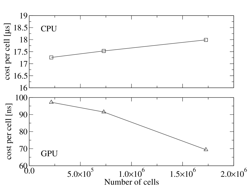
Figure 1: Cost per cell update for different problem sizes. The upper panel shows the CPU cost in microseconds, while the lower panel shows GPU cost (single precision) in nanoseconds. The CPU performance is almost independent of the problem size, while the GPU performs better with larger grids.

To investigate this, we calculate the computational cost per cell and iteration, and report the results in figure 1. A simple assumption of a machine’s performance scaling (that is, when we assume that only operation count is relevant for the cost) would imply that is number is almost constant when varying the grid size. From the plot, it is apparent that the CPU code almost has this property. However, the GPU becomes more efficient with larger problem size (i.e. a larger number of threads). It is therefore advisable to saturate the parallel processor as much as possible to obtain improved overall performance.

4.2 Relevance of disk output cost

	GPU (SP)	GPU (DP)
No output	132.50 s	635.54 s
With output	134.06 s	637.46 s
Relative cost	1.17 %	0.30 %

Table 3: Impact of disk output on GPU simulation performance, using an output frequency typical of a simulation performed in neutron star asteroseismology. GPU simulations have been performed in both single (SP) and double precision (DP), with the expectation that the relative cost is lower in double precision.

In this section, we consider the impact of disk output on the performance result. As discussed before, writing arbitrarily large quantities of data to disk would make the disk access the bottleneck in the problem, and in such a case neither CPU nor GPU speed may be very relevant. In contrast, we select a set of output parameters typical for our own scientific simulations (Zink et al., 2010) and observe the performance impact of the output. For this test, we evolve a neutron star for a time interval of $1\,\mathrm{ms}$ with a time step of $0.5\,\mu\mathrm{s}$. Output of overall norms (maximal value of density and similar) is performed every $5\,\mu\mathrm{s}$, whereas one-dimensional profile output along each axis, and also three-dimensional output of most evolution quantities, is performed every $50\,\mu\mathrm{s}$. The test is performed on a regular workstation with a SATA disk: a dedicated high-performance RAID system is expected to exhibit a smaller impact on performance. We report the results of the comparison in table 3. As can be seen, output does not substantially affect performance in this typical application case.

4.3 Performance on multiple GPUs

Horizon supports MPI parallelization, and therefore it is interesting to investigate the cost of scaling to multiple GPUs. At the time of writing, we have access to a dual Tesla C2070 setup inside a single workstation, and the following observations will therefore compare performance between a single and two GPUs.

We have tested the MPI scaling performance of Horizon using a grid size of $120\times 120\times 120$ for a single GPU, and $240\times 120\times 120$ for two GPUs. This choice comprises a weak scaling test, which should be appropriate in the present context since it excludes the grid-size dependent performance of the GPU (see figure 1) from the consideration of MPI messaging overhead measurements. The actual initial data is of little consequence in the measurement: because of the grid setup, we have opted for a Riemann problem.

	SP	DP
1 GPU	17.74 s	79.81 s
2 GPUs (MPI)	18.38 s	80.94 s
Parallel efficiency	96.5 %	98.6 %

Table 4: Cost of MPI parallelization (parallel efficiency), comparing a simulation running on two GPUs with a single GPU simulation, both in single (SP) and double precision (DP). This is a nontrivial test for GPUs even when only two MPI processes are used.

The results of the timing tests are reported in table 4. As for the disk output case, the parallel synchronization is a serial point inside the parallel program, and therefore could be a limiting factor by Amdahl’s law. However, in contrast to disk output, the MPI synchronization needs to be performed at every substep of the method to have a consistent global state. In principle, this could give rise to a substantial reduction in overall performance, but in the present case we observe good scaling efficiency. These results, while encouraging, are of course only partially indicative of parallel efficiency on a full cluster. However, given a particular (large) problem size, substantially less GPUs are needed to obtain the same performance as CPUs, thus requiring less MPI processes in comparison.

5 Comparison between single and double precision accuracy

This section will repeat selected standard test cases for GRMHD already performed with Thor using the GPU-accelerated Horizon code, with a focus on differences between single and double precision floating point accuracy. This is of particular interest as a consequence of the performance gap between these options, and whether a hybrid programming model, i.e. one that uses single precision accuracy in most operations and double precision in only selected ones, could be feasible. The results reported here use either pure single or double precision accuracy operations.

5.1 Shock tubes

We will first consider the Sod test (Sod, 1978), which is a standard test case for compressible hydrodynamics codes. We prepare a Riemann problem in an ideal gas with $\Gamma=5/3$, and with initial states $\rho_{L}=1$, $P_{L}=1$, $u^{i}_{L}=0$, and $\rho_{R}=0.125$, $P_{R}=0.1$, $u^{i}_{R}=0$. We prepare this problem on a full $120\times 120\times 120$ grid using Horizon, and simulate the evolution up to a time $t=0.8$. For comparison, a reference solution using Thor has been produced using a very fine grid.

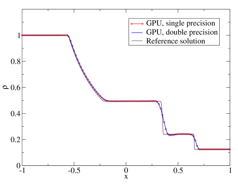
Figure 2: Sod test: comparison between single and double precision accuracy. This plot shows the density profile at time $t=0.8$. The GPU results were obtained with Horizon, whereas the reference solution is produced with Thor on a very fine grid.

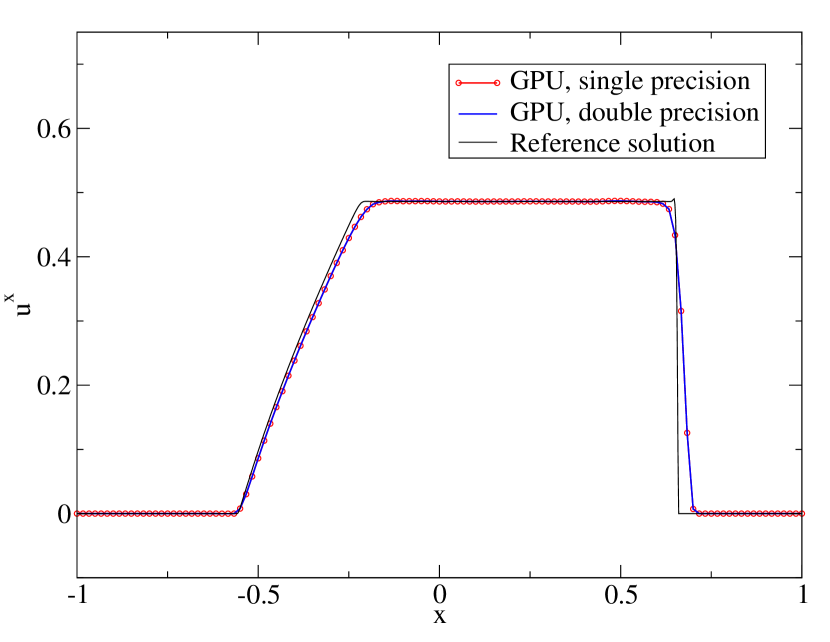
Figure 3: Same as figure 2, but comparing the x velocity $\tilde{u}^{x}$.

Figures 2 and 3 show the density and x-velocity profiles at the end of the evolution. The profiles show the somewhat dissipative nature of the HLL solver and TVD limiter we are using, but in particular, they show no discernible difference between single and double precision results. In fact, these differences are $|\delta\rho|\approx 5\times 10^{-5}$ and $|\delta\tilde{u}^{x}|\approx 10^{-4}$ exactly at the location of the shock, and typically $|\delta\rho|<1\times 10^{-6}$ and $|\delta\tilde{u}^{x}|<10^{-6}$ in smooth parts of the flow. These errors are at or lower than the level of the discretization error of the scheme.

A set of tests for magnetized flows have been proposed by Balsara (2001). We will show results from the first Balsara test, with initial data $\rho_{L}=1$, $P_{L}=1$, $u^{i}_{L}=0$, $B^{x}_{L}=0.5$, $B^{y}_{L}=1$, $B^{z}_{L}=0$, and $\rho_{R}=0.125$, $P_{R}=0.1$, $u^{i}_{R}=0$, $B^{x}_{R}=0.5$, $B^{y}_{R}=-1$, $B^{z}_{R}=0$. The setup is otherwise the same as for the Sod test.

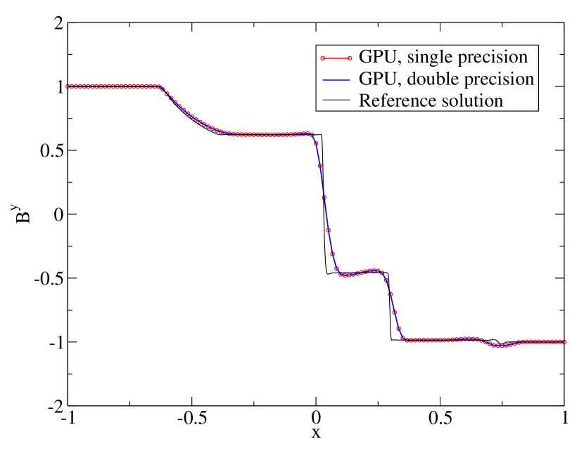
Figure 4: Balsara 1 test: comparison between single and double precision accuracy. This plot shows the magnetic field $B^{y}$ profile at time $t=0.8$. The GPU results were obtained with Horizon, whereas the reference solution is produced with Thor on a very fine grid.

In figure 4 we show a comparison of the magnetic field vector component $B^{y}$ (which is initially discontinuous) at the end of the evolution, as a representative quantity for comparison. As in the case of the Sod test, also the magnetic field structure is not significantly affected by using single precision accuracy, at least in this test case. The absolute differences between single and double precision are $|\delta B^{y}|<10^{-6}$, and similar statements hold for all other evolved quantities.

5.2 Oscillations in a rapidly rotating neutron star

A next comparison between single and double precision accuracy will be performed using a slightly perturbed stellar model. We use the model BU2 as in section 4.1, but additionally perturb it with a small quadrupole deformation ($\ell=2,m=0$) in order to analyze the dynamics of the star.

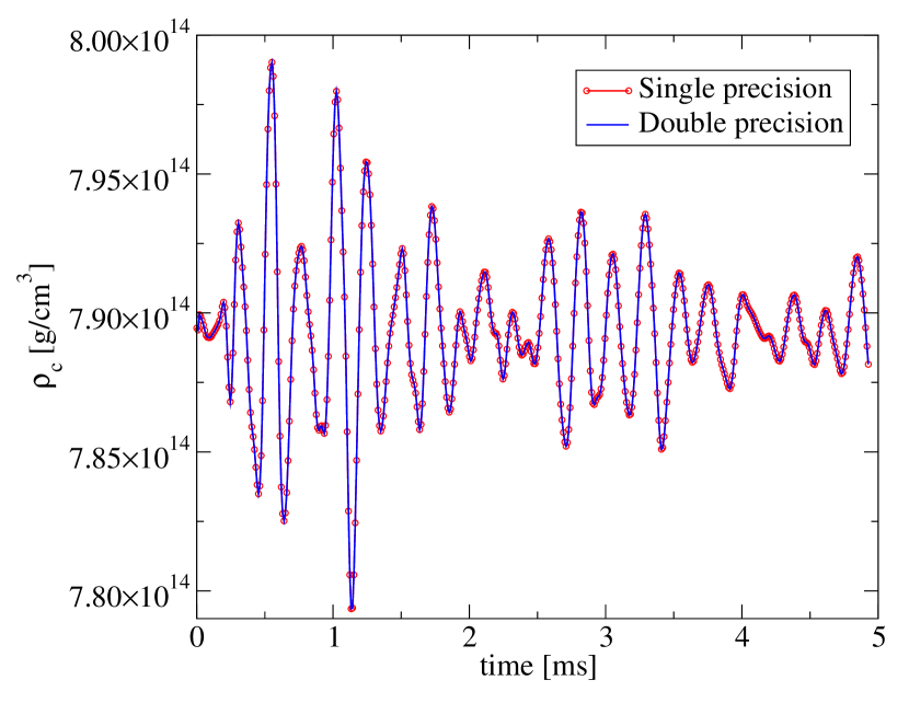
Figure 5: Oscillations of a rapidly rotating neutron star model: comparison between single and double precision evolutions using the Horizon code. This plot shows the central density of the star over a time of $5\,\mathrm{ms}$.

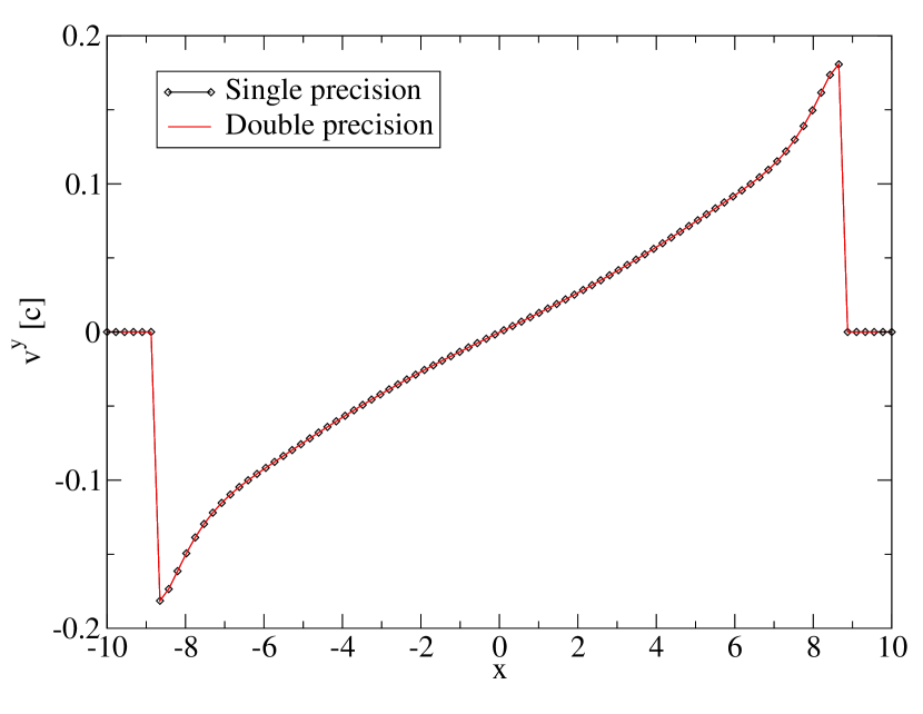
Figure 6: Oscillations of a rapidly rotating neutron star model: comparison between single and double precision evolutions using the Horizon code. This plot shows the evolved rotational velocity profile $\tilde{u}^{y}(x)$ after an evolution of $5\,\mathrm{ms}$.

The tests are performed with a moderate resolution ($90\times 90\times 90$, with about $60-70$ cells covering the stellar diameter), and we evolve the star for $5\,\mathrm{ms}$ physical time, corresponding to $10,000$ iterations. Figure 5 shows a comparison of the central density evolution using single and double precision simulations. As can be seen, the differences are very small, and likely smaller than the discretization error of the system. When transforming both time profiles into Fourier space (not shown here), we similarly get virtually identical spectra, and can identify the fundamental radial mode $F$ at $2596\pm 30\,\mathrm{Hz}$, its overtone $H_{1}$ at $4403\pm 30\,\mathrm{Hz}$, the fundamental quadrupole mode ${}^{2}f$ at $1909\pm 30\,\mathrm{Hz}$, and its overtone ${}^{2}p_{1}$ at $3970\pm 30\,\mathrm{Hz}$. These numbers match very well with Gaertig & Kokkotas (2008), but specifically, there is no discernible difference between the single and double precision results.

Another very sensitive quantity is the rotational velocity profile of the star. In figure 6, we compare the x-axis profile of $\tilde{u}^{y}(x)$ after $5\,\mathrm{ms}$. Again, virtually no differences between single and double precision results are apparent, even in the problematic region near the stellar surface. The maximal deviation is $|\delta\tilde{u}^{y}|<5\times 10^{-6}$.

We conclude that, at least for the applications presented here, single precision calculations should be sufficient. However, as with all other parameters entering a numerical calculation (discretization scheme, time step, spatial resolution, …), this assumption must be tested on a case-by-case basis. We will further discuss this point below.

5.3 Strongly magnetized neutron star

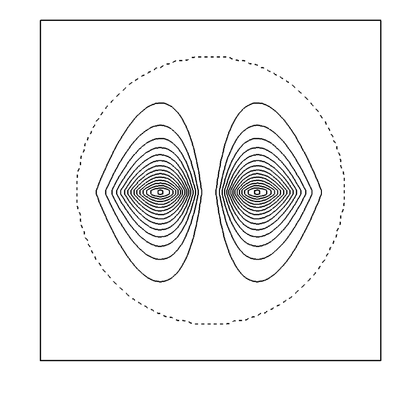
Figure 7: Strongly magnetized neutron star: Initial distribution of the amplitude of the magnetic field within a meridional cut, with contours up to about $2\times 10^{15}\,\mathrm{G}$. The dashed line denotes the stellar surface.

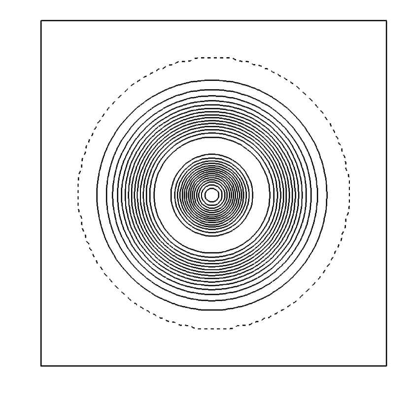
Figure 8: Same as figure 7, but inside the equatorial plane of the star.

As a final point of comparison we explore a magnetized neutron star model. For this test, we use the nonrotating model BU0 (Dimmelmeier et al., 2006), which is defined by $\rho_{c}=1.28e-3$ and $\Gamma=2$ and has a mass of $M=1.4\,M_{\odot}$. On this model, we superimpose a toroidal magnetic field given by (Braithwaite, 2006)

$$\mathbf{B}=B_{0}\left(\frac{\varpi}{\varpi_{0}}\right)^{2}e^{-\varpi^{2}/\varpi_{0}^{2}}e^{-z/2H}\mathbf{e}_{\phi}$$ (4)

where $\varpi=\sqrt{x^{2}+y^{2}}$, and we choose $\varpi_{0}=3$, $H=1$, and $B_{0}$ such that the maximal field strength is approximately $2.6\times 10^{15}\,\mathrm{G}$. The structure of the initial magnetic field is shown in figures 7 and 8.

Even with these comparatively high field strengths, the magnetic field is only a small perturbation to the fluid equilibrium. It is also known that this field is unstable Braithwaite (2006); Lander & Jones (2010); Duez et al. (2010), but we will only be concerned here with differences between single and double precision evolutions. As in the previous section, we evolve the model for $5\,ms$ physical time on a $90\times 90\times 90$ grid.

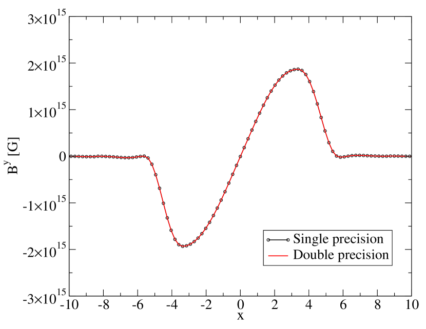
Figure 9: Strongly magnetized neutron star: Comparison between single and double precision evolutions. This plot shows the profile $B^{y}(x)$ after an evolution of $5\,\mathrm{ms}$.

Figure 9 shows the profile $B^{y}(x)$ at the end of the evolution from both simulations. The disagreement is within $|\delta B|<10^{12}\,\mathrm{G}$, and therefore larger than in the non-magnetized case, but still well below $10^{-3}$ of the actual field strength.

6 Discussion

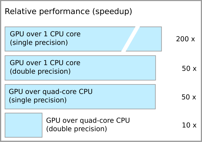
Figure 10: Relative performance of the GPU-based Horizon code compared to the CPU-based Thor code. These numbers approximately represent the timing results obtained in section 4, which have been measured with an Intel Xeon E5620 CPU and an NVIDIA Geforce GTX580 GPU. The first number is the one typically used in publications on GPU codes, whereas the third and fourth row show more realistic comparisons between a parallel code running on a GPU and a parallel code running on a quad-core CPU. In section 5 we have presented results indicating that single precision accuracy may be sufficient for a number of applications. Further discussion of this point can be found in the text.

This paper describes an implementation of general relativistic magnetohydrodynamics on graphics processing units, the Horizon code, and presents results on the relative performance practitioners can expect to gain from employing GPUs in such a context. The main results from performance measurements, obtained in a setup which is close to applications in neutron star asteroseismology, are summarized in figure 10.

We have argued that general relativistic magnetohydrodynamics should map very well to GPUs as a consequence of the data-parallel nature of the problem, mostly regular memory access patterns, and a higher arithmetic intensity than is common in traditional Newtonian MHD codes. Timing tests have confirmed this expectation, and have shown substantial performance gains over current CPU architectures. We have selected a particular CPU/GPU combination for these tests, but this general picture will not change when comparing different sets of current hardware implementations, even though the actual speedup numbers will vary.

From an astrophysical application perspective, we can expect about an order of magnitude increase in performance by employing a double precision GPU calculations in place of a quad-core CPU, and several orders of magnitude when employing only single precision arithmetics. This is a direct consequence of the massively parallel, high-throughput nature of the GPU, and the fact that GRMHD maps well to this kind of architecture.

Given the often very demanding problems which result from implementation of astrophysical models, and the high cost of three-dimensional explicit simulations, an order of magnitude in performance should be enough of an incentive to consider GPUs, and similar massively parallel architectures, in place of CPUs. Such a performance gain is interesting to attack substantially larger simulations (or longer evolution times) on compute clusters, provided a GPU-based machine is available.

However, another use of GPUs should be mentioned which is no less important in practice: the ability to perform reasonably sized full-scale simulations on a single workstation, with a high turnaround time for results. This is relevant to explore new numerical methods and model parameters spaces, which can now be performed much faster, and much more conveniently, than using many nodes on a cluster resource. In this way, scientific productivity can be gained very easily with a modest investment in hardware.

The much higher throughput obtained in single precision computations begs the question whether computations could also be performed with a reduced level of accuracy. We would first like to stress that this aspect of course also applies to the distinction between double and quadruple precision, and there may well be problems for which even double precision is not sufficient. Overall, this is entirely dependent on the particular problem and numerical algorithm employed, and only experimentation can establish whether a particular floating point approximation is sufficient. Of course, this equally applies to all other free parameters of the discretization.

In the particular cases we have investigated here, which consider shock tubes, small oscillations of rotating stars, and strongly magnetizes stars, it seems that single precision floating point accuracy could be sufficient for a number of modeling purposes. That statement may well cease to be true if tabulated equations of state, turbulence, radiation transport, reaction networks etc. are involved in a calculation. If such is the case, a good strategy could be to locate (approximately) the components of the numerical code which should require double precision accuracy, and then employ the higher accuracy only in these parts. Horizon offers exactly this option by allowing to adjust the accuracy of the conservative to primitive variable transformation and the calculation of flux differences. Such a hybrid approach could preserve very high levels of performance while keeping the required level of accuracy.

But the most important aspect of GPU computation, and more generally, massively data-parallel hardware architectures (which may also be located on a CPU), are not the potential gains which could be achieved at the present time: it is the fact that the peak performance in these hardware designs grows much more rapidly than the peak performance of traditional CPUs. That is, the relative factor of 10 we can achieve today may translate into a factor of 20 in two years time. Preparing for this major shift in high-performance architecture, which is not only driven by the isolated requirements of a small market segment as in the past, but pervades the global development of all consumer and professional-level microprocessors, should be considered a priority for future computational tools in astrophysics.

References

- Amdahl (1967) Amdahl, G. M. 1967, in Proceedings of the 1967 Spring Joint Computer Conference, AFIPS ’67 (New York: ACM), 483–485
- Anderson et al. (2006) Anderson, M., Hirschmann, E., Liebling, S. L., & Neilsen, D. 2006, Class. Quantum Grav., 23, 6503
- Antón et al. (2006) Antón, L., Zanotti, O., Miralles, J. A., Martí, J. M., Ibáñez, J. M., Font, J. A., & Pons, J. A. 2006, Astrophys. J., 637, 296
- Balsara (2001) Balsara, D. 2001, ApJS, 132, 83
- Banyuls et al. (1997) Banyuls, F., Font, J. A., Ibáñez, J. M., Martí, J. M., & Miralles, J. A. 1997, Astrophys. J., 476, 221
- Barsdell et al. (2010) Barsdell, B. R., Barnes, D. G., & Fluke, C. J. 2010, arXiv:1001.2048
- Belleman et al. (2008) Belleman, R. G., Bédorf, J., & Portegies Zwart, S. F. 2008, New A, 13, 103
- Braithwaite (2006) Braithwaite, J. 2006, A&A, 453, 687
- Bucciantini & Del Zanna (2010) Bucciantini, N., & Del Zanna, L. 2010, arXiv:1010.3532
- Cerdá-Durán et al. (2008) Cerdá-Durán, P., Font, J. A., Antón, L., & Müller, E. 2008, A&A, 492, 937
- Choudhary et al. (2010) Choudhary, N. K., Ginjupalli, R., Navada, S., & Khanna, G. 2010, arXiv:1010.3816
- De Villiers & Hawley (2003) De Villiers, J., & Hawley, J. F. 2003, ApJ, 589, 458
- Del Zanna et al. (2007) Del Zanna, L., Zanotti, O., Bucciantini, N., & Londrillo, P. 2007, A&A, 473, 11
- Dimmelmeier et al. (2006) Dimmelmeier, H., Stergioulas, N., & Font, J. A. 2006, MNRAS, 368, 1609
- Duez et al. (2010) Duez, V., Braithwaite, J., & Mathis, S. 2010, ApJ, 724, L34
- Etienne et al. (2010) Etienne, Z. B., Liu, Y. T., & Shapiro, S. L. 2010, Phys. Rev. D, 82, 084031
- Fluke et al. (2010) Fluke, C. J., Barnes, D. G., Barsdell, B. R., & Hassan, A. H. 2010, arXiv:1008.4623
- Font (2008) Font, J. A. 2008, Living Reviews in Relativity, 11, 7
- Gaertig & Kokkotas (2008) Gaertig, E., & Kokkotas, K. D. 2008, Phys. Rev. D, 78, 064063
- Gammie et al. (2003) Gammie, C. F., McKinney, J. C., & Tóth, G. 2003, Astrophys. J., 589, 444
- Garland & Kirk (2010) Garland, M., & Kirk, D. 2010, Comm. of the ACM, 53, 58
- Giacomazzo & Rezzolla (2006) Giacomazzo, B., & Rezzolla, L. 2006, Journal of Fluid Mechanics, 562, 223
- Giacomazzo & Rezzolla (2007) Giacomazzo, B., & Rezzolla, L. 2007, Class. Quantum Grav., 24, S235
- Harten et al. (1983) Harten, A., Lax, P. D., & van Leer, B. 1983, SIAM Rev., 25, 35
- Herrmann et al. (2010) Herrmann, F., Silberholz, J., Bellone, M., Guerberoff, G., & Tiglio, M. 2010, Classical and Quantum Gravity, 27, 032001
- Khanna & McKennon (2010) Khanna, G., & McKennon, J. 2010, Computer Physics Communications, 181, 1605
- Kirk & Hwu (2010) Kirk, D., & Hwu, W. 2010, Programming Massively Parallel Processors (Morgan Kaufmann)
- Klöckner et al. (2009) Klöckner, A., Warburton, T., Bridge, J., & Hesthaven, J. S. 2009, Journal of Computational Physics, 228, 7863
- Koide et al. (1999) Koide, S., Shibata, K., & Kudoh, T. 1999, ApJ, 522, 727
- Komissarov (2004) Komissarov, S. S. 2004, Mon. Not. R. Astron. Soc., 350, 1431
- Korobkin et al. (2010) Korobkin, O., Abdikamalov, E. B., Schnetter, E., Stergioulas, N., & Zink, B. 2010, arXiv:1011.3010
- Lander & Jones (2010) Lander, S. K., & Jones, D. I. 2010, MNRAS, 1884
- Martí & Müller (1999) Martí, J. M., & Müller, E. 1999, Living Rev. Relativity, 2, 3
- Mizuno et al. (2006) Mizuno, Y., Nishikawa, K., Koide, S., Hardee, P., & Fishman, G. J. 2006, arXiv:astro-ph/0609004
- Noble et al. (2006) Noble, S. C., Gammie, C. F., McKinney, J. C., & Del Zanna, L. 2006, ApJ, 641, 626
- Pang et al. (2010) Pang, B., Pen, U., & Perrone, M. 2010, arXiv:1004.1680
- Portegies Zwart et al. (2007) Portegies Zwart, S. F., Belleman, R. G., & Geldof, P. M. 2007, New A, 12, 641
- Schive et al. (2008) Schive, H., Chien, C., Wong, S., Tsai, Y., & Chiueh, T. 2008, New A, 13, 418
- Sod (1978) Sod, G. A. 1978, Journal of Computational Physics, 27, 1
- Stergioulas & Friedman (1995) Stergioulas, N., & Friedman, J. L. 1995, Astrophys. J., 444, 306
- Wang (2009) Wang, P. 2009, PhD thesis, Stanford University
- Wang et al. (2010) Wang, P., Abel, T., & Kaehler, R. 2010, New A, 15, 581
- Wong et al. (2009) Wong, H., Wong, U., Feng, X., & Tang, Z. 2009, arXiv:0908.4362
- Yamamoto et al. (2008) Yamamoto, T., Shibata, M., & Taniguchi, K. 2008, Phys. Rev. D, 78, 064054
- Zink (2008) Zink, B. 2008, in CCT Technical Reports, TR-2008-1
- Zink et al. (2010) Zink, B., Korobkin, O., Schnetter, E., & Stergioulas, N. 2010, Phys. Rev. D, 81, 084055
- Zink et al. (2008) Zink, B., Schnetter, E., & Tiglio, M. 2008, Phys. Rev. D, 77, 103015