Rapid non-adiabatic loading in an optical lattice

Abstract

We present a scheme for non-adiabatically loading a Bose-Einstein condensate into the ground state of a one dimensional optical lattice within a few tens of microseconds typically, i.e. in less than half the Talbot period. This technique of coherent control is based on sequences of pulsed perturbations and experimental results demonstrate its feasibility and effectiveness. As the loading process is much shorter than the traditional adiabatic loading timescale, this method may find many applications.

.

Numerous works related to optical lattice trapping have been published, especially using coherent atoms or Bose-Einstein condensate (BEC) RMP06 , since it has various applications in quantum computation, simulation of basic condensed matter physics, atomic clocks, etc. A common concern to those experiments is how to load a BEC into the lattice without excitation or heating PRA03 ; PRA04 ; PRA05 . In most cases, one chooses to turn on the light field adiabatically and the loading process usually lasts up to tens of milliseconds, during which one tries to avoid excitations to higher states. A long loading may be problematic for quantum computation experiments as it increases the time during which decoherence can occur and reduces speed when atoms stored in optical lattices shall be interrogated and reloaded several times. Furthermore, adiabatic loading is difficult to obtain near the critical point of phase transitions for finite temperatures even well bellow the BEC critical temperature.

An alternative idea is to prepare the BEC in the ground state of the lattice, and then turn on the lattice suddenly. This ’preparing’ process can be much shorter compared to the adiabatic loading (about $30\ \mu s$, as we can see later in this article). One way for realizing this ’preparing’ process can stem from nonholonomic coherent control PhysRevLett.75.346 ; PhysRevLett.82.1 ; EPJ06 . In this approach, a sequence of two well chosen Hamiltonians are imposed on the system and the preset duration of each step is modified according to a defined cost function, in order to get the aimed evolution operator as well as the target state.

Our proposal for designing and computing the pre-loading process is reminiscent of this method, but we focus more on the feasibility of its experimental implementation, rather than the stringency or universality of the approach. Experimentally, we achieve the non-adiabatic loading with a very few pulses using directly the results of our computational design. According to our analysis, this method would be valid on many other occasions, such as loading the condensate directly into excited states of the lattice. We first introduce a general method for determining the sequence of steps to be applied to the system before giving an account of our experimental results.

Suppose that before the sudden loading at time $t_{0}$ of the lattice with optical depth $V_{0}$, $m$ steps have been applied. The $i$th step corresponds to a Hamiltonian $\hat{H}_{i}$ kept constant during $t_{i}$. The final state $|\psi(t_{0})\rangle$ is given by:

$$\centering|\psi(t_{0})\rangle=\prod_{i=m}^{1}\hat{U}_{i}|\psi_{0}\rangle\@add@centering$$ (1)

where $\hat{U}_{i}=e^{-i\hat{H}_{i}t_{i}/\hbar}$ is the evolution operator of the $i$th process. With $|\psi_{a}\rangle$ the aimed state, which is the ground state of the lattice in the context of this paper, the total population of the excited states $N_{e}$ at time $t_{0}$, is:

$$\centering N_{e}=1-|\langle\psi_{a}|\psi(t_{0})\rangle|^{2}\@add@centering$$ (2)

Our goal is to properly choose $\hat{H}_{i}$ and $t_{i}$ so that $N_{e}$ is small enough to be neglected in the experiment, or the final state $|\psi(t_{0})\rangle$ to be close enough to $|\psi_{a}\rangle$.

The target state $|\psi_{a}\rangle$ can be obtained simply if atomic interactions are neglected. The effect of the optical lattice on the atoms corresponds to a stationary periodical potential with periodicity $\lambda_{L}/2$, spontaneous emission being neglected since the laser used for the lattice is sufficiently far detuned. So neglecting atomic interactions, the Hamiltonian of the interaction of atoms with the optical lattice is:

$$\centering\hat{H}_{0}=\frac{\hat{p}^{2}}{2m}+\frac{V_{0}}{2}(1+\cos{2k_{L}x})\@add@centering$$ (3)

where $m$ is the atom mass, $k_{L}$ is the wave number of lattice light and $V_{0}$ the lattice depth and $\hat{p}$ is the momentum of each atom. The corresponding Talbot time Deng99 is $T_{T}=\frac{2\pi}{4\omega_{R}}$, where $\omega_{R}=\frac{\hbar k_{L}^{2}}{2m}$ is the one photon recoil frequency. Because of the periodicity of the potential, $|\psi_{a}\rangle$ can be decomposed over a reduced basis of plane waves $|2n\hbar k_{L}\rangle$. One obvious choice for each $\hat{H}_{i}$ is to take the Hamiltonian corresponding to the interaction of atoms with a standing wave with same periodicity $\lambda_{L}/2$ so that the Hilbert space is limited to the basis of states $|2n\hbar k_{L}\rangle$. For this purpose, the power of the same laser as the one used for the final lattice loading is simply adjusted and each Hamiltonian $\hat{H}_{i}$ is obtained from Eq. (3) after substitution of $V_{0}$ by the new lattice depth $V_{i}$.

More precisely, as $\hat{H}_{i}$ has spatial periodicity, we get its eigenstates by solving the equation $\hat{H}_{i}|n,q\rangle=E_{n,q}|n,q\rangle$ JPB02 , where $|n,q\rangle$ is a Bloch state with $n$ the band index and $q$ the quasi momentum and $E_{n,q}$ is the corresponding eigenenergy. We use the notation $|n,q,V_{i}\rangle$ for denoting the Bloch states for a $V_{i}$ lattice depth. Since only Bloch State with $q=0$ is populated initially, no other quasimomenta can be populated during the sequence of pulses. Thus the state of the system can be spanned over the momentum eigenstates basis $|2{\ell}\hbar k_{L}\rangle$, independent on the potential depth $V_{i}$ and the evolution operator can be written as the following matrix: $\mathbf{U}_{i}(V_{i},t_{i})=\mathbf{C}(V_{i})\mathbf{E}(V_{i},t_{i})\mathbf{C}(V_{i})^{\dagger}$, where $\mathbf{C}(V_{i})$ is the unitary matrix of transition between the Bloch States basis and the momentum eigenstates basis with matrix elements $\mathbf{C}(V_{i})_{{\ell}n}=\langle 2{\ell}\hbar k_{L}|n,q=0,V_{i}\rangle$ and where $\mathbf{E}(V_{i},t_{i})$ is a diagonal matrix with elements $\mathbf{E}(V_{i},t_{i})_{nn}=\exp(-iE_{n,q=0}(V_{i})t_{i}/\hbar)$. Because of the simple form of the potential, these matrices are easily obtained and from those the wave function’s evolution is solved numerically.

A traditional simple approximation to solve this problem of a standing wave of light pulse interaction with atoms is to omit the effect of kinetic energy. As shown in the works Deng99 ; Clark10 , the motional term in the Hamiltonian may be neglected. For a square pulse, when the depth of the standing wave potential is $V$ and the duration of the pulse is $t$, the wave function after the pulse can be expressed as $\psi(t)=\psi(0)e^{-i\frac{V\cdot t}{2\hbar}\cos{2k_{L}x}}$ and decomposed over different momentum states $|2n\hbar k_{L}\rangle$, using the Bessel functions. This approximation is valid only in the Raman-Nath regime, when the pulse is short enough that the displacement of the atoms is much smaller than the lattice period. From references PRL99 ; NJP09 , we can see experimental data deviate distinctly from the Bessel functions when the pulse duration is longer. For multi pulse cases, the motion term may be neglected during each pulse but taken into account during the intervals between pulses. This approximation is valid only when the sum of all the pulses’ durations is far less than the Talbot time $T_{T}$. In Deng99 , $T_{T}=10\ \mu$s, and two $100\ ns$ pulses were applied, while the interval time can be up to $10\ \mu$s. However, as the total pulse duration $200\ ns$ is far less than $T_{T}$, the whole process is still in Raman-Nath regime and we can see the theoretical prediction agrees well with the experimental results.

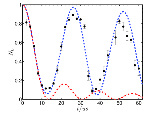
Figure 1: (color online) Relative atom number $N_{0}$ in $p=0\hbar k_{L}$ mode versus the pulse duration $t$ of a single standing-wave pulse applied to the system. The black points with error bars are experimental data and the red dashed-dotted line is calculated with the simple method where the kinetic energy is neglected while the blue dashed line is given by the general method (see text).

We compare in Fig. 1 the results of the two methods with our experimental data for the case of a single square pulse applied to the system. In our experiment, we first prepare a BEC of about $2\times 10^{5}$ ⁸⁷Rb atoms in the $|F=2,m_{F}=2\rangle$ hyperfine ground state in the magnetic trap, with longitudinal length $L=100\ \mu$m and width $l=10\ \mu$m Zhou10 . The BEC is then loaded into a one-dimensional optical lattice with light wavelength $\lambda_{L}=852$ nm, along its axial direction. We suddenly turn on the standing-wave potential to a specific depth, hold the lattice for different durations $t$, release the condensate and measure the relative atom number $N_{0}$ in $p=0\hbar k_{L}$ mode. Without considering the atomic motion, the Bessel function (red dashed-dotted line) failed to fit the experiment data when $t$ is larger than about $10\ \mu$s. On the other hand, the numerical solution taking the motional term into account (blue dashed line) predicts the experiment accurately up to $60\ \mu$s, although some other effects have been neglected, such as interaction between atoms and non-zero momentum width of the condensate. As a result, we will use the general method as it will impose less restriction on our sequence design. Note that $T_{T}\approx 79\ \mu$s in our configuration and the fitted potential depth is $18E_{R}$, where $E_{R}=(\hbar k_{L})^{2}/2m$ is the one photon recoil energy.

In a first attempt to design the time sequence, we use four steps, each corresponding to the application of a potential with depth $V_{i}$ and a duration $t_{i}$ as shown in Fig. 2a. Thus, from these eight free parameters ${V_{i},t_{i}}$ with $i=1$ to 4, we can obtain the evolution operators ${\mathbf{U}_{i}}$ and the exciting rate $N_{e}$ according to our previous analysis. If we want to get the minimum of $N_{e}$, it requires to test all the combinations of the eight free parameters and need too much computing time. However, we find convergence to a local minimum is easy to obtain. For this purpose we modify the parameters step by step, with a small change of one parameter every step, in order to get a smaller $N_{e}$. If no smaller result for $N_{e}$ can be obtained by changing any of these parameters, the minimization of $N_{e}$ is stopped and the corresponding combination of parameters is the result of our design. Note that different initial values of the parameters may result in different local minima. Actually we try more than one group of initial parameters in order to get a better result, though the optimized pulse sequences obtained for different and often lower lattice depths are already good input values. As shown in Fig. 2c, the exciting rate $N_{e}$ remains lower than $0.1\%$. The whole pre-loading process lasts for about $30\ \mu$s, which is beyond the Raman-Nath Regime but still within the limit of our method.

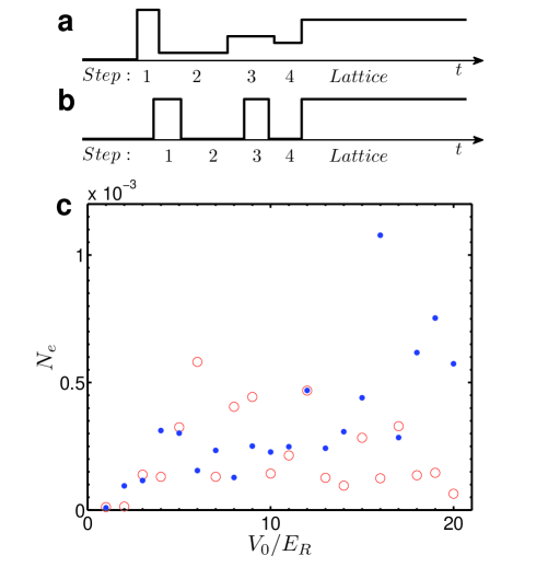
Figure 2: (color online) Two schemes for the non-adiabatic loading. (a) Four steps pre-loading sequence with both the potential depth and the duration of each step set as free parameters. (b) Four steps pre-loading sequence with fixed potential depth and variable duration in each step. (c) Corresponding relative population $N_{e}$ in excited Bloch states as a function of lattice depth, with red circles for scheme (a) and blue points for scheme (b).

Nevertheless, it is not easy for this scheme to be experimentally implemented. As the lattice depth varies with time, we need a feed back loop to control the laser power to get a stable optical lattice as the atoms are very sensitive to fluctuation of the laser power. We also need sharp rising and falling edges to ensure each step duration is sufficiently similar to the designed one. If $0.5\ \mu$s is set for the upper limit of each rising and falling edge, the bandwidth of the power controlling loop should be larger than $1$ MHz, which is hard to achieve. We would rather choose the scheme illustrated in Fig. 2b, where the step $V_{1}$ and $V_{3}$ are fixed at $V_{0}$, and the step $V_{2}$ and $V_{4}$ are fixed at $0$, $t_{i}$ still being free parameters. This means no feed back loop but only a switch is needed so that the rising and falling time can be decreased to $200\ ns$ easily. In Fig. 2c, we can see the exciting rate is still lower than $0.1\%$ for most lattice depths lower than $20\ E_{R}$, although some degrees of freedom of our sequence of pulses are locked. In TABLE I we show the designed time sequences for several lattice depths.

Table 1: Time duration of each step $t_{i}$ ($\mu$s) for different lattice depths $V_{0}$ with unit $E_{R}$.

$V_{0}$	$t_{1}$	$t_{2}$	$t_{3}$	$t_{4}$	$t_{5}$	$t_{6}$	$t_{7}$	$t_{8}$
4	10	9.5	4	5	6	5	9	9
8	6.5	10.5	5	6	6	4.5	10.5	7
12	5	11.5	4.5	6	5.5	4	11.5	5.5
16	4.5	12	3.5	6	5	4	12.5	4.5
20	3.5	13	3.5	5.5	6	3.5	12.5	3.5

Furthermore, we can transfer the state $|\psi_{a}\rangle$ back to the initial state $|\psi_{0}\rangle$ after releasing the lattice, using a similar process. TABLE I gives also the designed sequence, with time durations $t_{5}$ to $t_{8}$ and corresponding potentials, $V_{5}$ and $V_{7}$ being set to $0$, while $V_{6}$ and $V_{8}$ equal to $V_{0}$ (see Fig. 3b). Note that this sequence is equivalent to the timely inverted pre-loading sequence if we ignore some minor deviations.

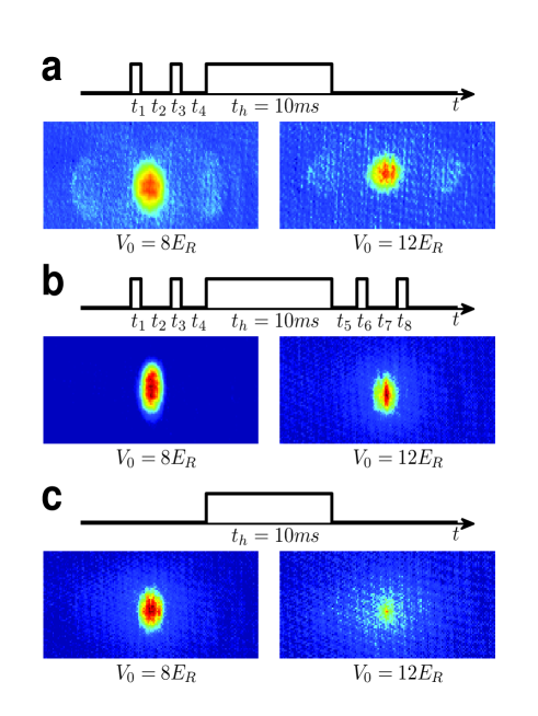
Figure 3: (color online) Absorption images for three different time sequences. As the condensate was released from both the lattice potential and the magnetic trap, it expands freely for $30ms$ and then an absorption image is taken. For each time sequence, we show the results for two lattice depths of $8E_{R}$ and $12E_{R}$.

To demonstrate the feasibility of our proposal, we did the experiment according to three different schemes. In the first scheme (Fig. 3a), we non-adiabatically load the BEC into the lattice, according to the designed process, hold it in the lattice for $t_{h}=10\ ms$ and release the atoms. We can see the interference peaks, similar to the familiar pattern observed in adiabatic loading experiments, which indicates a successful loading without significant excitation and heating. In the second scheme (Fig. 3b), after the same loading and holding process, we use two additional pulses to transfer the atoms back to the original state $|\psi_{0}\rangle$. Compared with the third scheme (Fig. 3c), where we directly turn on and off the lattice light without the pre-loading or post-releasing processes to prevent excitation but hold for the same period, the second scheme has little heating or disturbing effect on our BEC, which proves the effectiveness of our ’preparing’ process of the lattice ground state. A small heating may still be observed at $12E_{R}$. It may be due to interaction between atoms which are not included in our model.

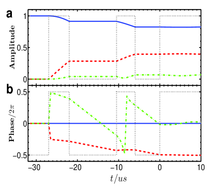
Figure 4: (color online) Evolution of the different momentum components of the wave function. Amplitude (a) and phase (b) for the $p=0\hbar k_{L}$, $\pm 2\hbar k_{L}$ and $\pm 4\hbar k_{L}$ modes are shown with blue solid lines, red dashed lines and green dashed-dotted lines respectively. The black dotted lines in both figures indicate the corresponding time sequence of the standing wave potential.

Fig. 4 shows the evolution of the wave function under a pulsed scheme shown in Fig.2b. We can see that atoms can be transferred between different momentum orders only when the pulse is on. In the intervals, the amplitudes of different components keep constant, while the phases vary linearly. The phase of the $\pm 4\hbar k_{L}$ order evolves four times faster than that of $\pm 2\hbar k_{L}$ as the kinetic energy is four times lager. After switching on the optical lattice ($t=0\ \mu$s), the amplitude and phase of all components keep almost unchanged as the wave function is in the ground state of the lattice. Note that the phase jump of the non-zero momentum components at $t=-27\ \mu$s is not significant since the amplitude of these components before that time is zero.

By simply replacing the initial state $|\psi_{0}\rangle$ and the aimed state $|\psi_{a}\rangle$, our pulse sequence design is also applicable to other situations. For example, by setting $|\psi_{0}\rangle=|n=0,q=0,V_{1}\rangle$ and $|\psi_{a}\rangle=|n=0,q=0,V_{2}\rangle$, we can get a process that can change the lattice depth from $V_{1}$ to $V_{2}$ non-adiabatically without excitation. We can also load the BEC directly to symmetric excited states such as $|n=2,q=0\rangle$, by setting them as $|\psi_{a}\rangle$. Our numerical simulation shows when $V_{0}$ is around $12\ E_{R}$, there exists theoretical possibility to load more than $99\%$ of the atoms to $|n=2,q=0\rangle$. This state can be used for studying spontaneous transition from high lying Bloch bands to lower bands experimentally. If the optical lattice is accelerated, anti-symmetric states and states with $q\neq 0$ could also be loaded.

In general, our method can be used to produce states whose momentum components are discrete and separated equally by $2\hbar k_{L}$. For example, we can divide one BEC into two momentum modes $|\pm 2m\hbar k_{L}\rangle$ equally, with negligible population in other orders. This technique is useful in atom interferometry and its theory has been developed in reference Clark10 , while neglecting the motional term in the Hamiltonian, as discussed earlier in this article. Our method is not restricted by the Raman-Nath regime and thus gives more freedom for designing the pulse sequence.

In conclusion, we proposed a method reminiscent of the nonholonomic coherent control technique for loading the BEC into one dimensional optical lattice non-adiabatically, within a much shorter loading time (usually less than $T_{T}/2$) than the commonly applied adiabatic method (much longer than $T_{T}$). Our experimental results demonstrate the validity of this method. We claim that this numerical design process can be applied to various topics related to the interaction of a standing wave of light with ultra-cold gases.

This work is supported by NKBRSFC(2011CB921501) and NSFC(61027016,61078026,10874008 and 10934010).

References

- (1) S. Lloyd, Phys. Rev. Lett. 75, 346 (1995);
- (2) G. Harel, and V. M. Akulin, Phys. Rev. Lett. 82, 1 (1999);
- (3) O. Morsch, M. Oberthaler, Rev. Mod. Phys. 78, 179 (2006);
- (4) A. S. Mellish, G. Duffy, C. McKenzie, R. Geursen, and A. C. Wilson, Phys. Rev. A 68, 051601 (2003);
- (5) P. B. Blakie and J. V. Porto, Phys. Rev. A 69, 013603 (2004);
- (6) P. S. Julienne, C. J. Williams, Y. B. Band, and Marek Trippenbach, Phys. Rev. A 72, 053615 (2005);
- (7) E. Brion, D. Comparat and G. Harel, Eur. Phys. J. D 39, 381 (2006);
- (8) L. Deng, E. W. Hagley, J. Denschlag, J. E. Simsarian, M. Edwards, C. W. Clark, K. Helmerson, Phys. Rev. Lett. 83, 5407 (1999);
- (9) J. H. Denschlag, J. E. Simsarian, H. Haffner, C. McKenzie, A. Browacys, D. Cho, K. Helmerson, S. L. Rolston and W. D. Phillips, J. Phys. B: At. Mol. Opt. Phys. 35, 3095 (2002);
- (10) M. Edwards, B. Benton, J. Heward and C. W. Clark, arXiv: 1009.0759v2 (2010);
- (11) R. E. Sapiro1, R. Zhang and G. Raithel, New Jour. Phys. 11, 013013 (2009);
- (12) Y. B. Ovchinnikov, J. H. Muller, M. R. Doery, E. J. D. Vredenbregt,K. Helmerson, S. L. Rolston, and W. D. Phillips, Phys. Rev. Lett. 83, 284 (1999);
- (13) X. J. Zhou, F. Yang, X. G., T. Vogt, and X. Z. Chen, Phys. Rev. A 81, 013615 (2010).