Screening bulk curvature in the presence of large brane tension

Abstract

We study a flat brane solution in an effective $5D$ action for cascading gravity and propose a mechanism to screen extrinsic curvature in the presence of a large tension on the brane. The screening mechanism leaves the bulk Riemann-flat, thus making it simpler to generalize large extra dimension dark energy models to higher codimensions. By studying an action with cubic interactions for the brane-bending scalar mode, we find that the perturbed action suffers from ghostlike instabilities for positive tension, whereas it can be made ghost-free for sufficiently small negative tension.

I Introduction

The problem of cosmic acceleration and its possible explanation as a cosmological constant have led to a wide variety of models in theoretical physics. Higher-dimensional theories of dark energy, in which our Universe is viewed as a $4D$ brane living in a higher-dimensional bulk, offer an interesting proposal towards understanding dark energy as a manifestation of the presence of extra dimensions of space-time. Much progress has been made in this field using the braneworld picture in which all standard model particles are confined to a $4D$ brane, while gravity is free to explore the bulk Lukas et al. (1999); Arkani-Hamed et al. (1998); Antoniadis et al. (1998). This makes it possible to have cosmologically large extra dimensions Arkani-Hamed et al. (1998); Randall and Sundrum (1999a, b). The Dvali-Gabadadze-Porrati (DGP) model Dvali et al. (2000), in particular, takes this idea to the extreme and considers our $4D$ Universe to be embedded in a $5D$ bulk of infinite extent. Despite being observationally disfavored Rydbeck et al. (2007); Fang et al. (2008); Lombriser et al. (2009); Guo et al. (2006), the normal branch of the DGP model is perturbatively ghost-free, in contrast to the self-accelerating branch Nicolis and Rattazzi (2004); Koyama (2005); Gorbunov et al. (2006); Charmousis et al. (2006); Dvali et al. (2007a); Gregory et al. (2007), and thus represents a perturbatively consistent infrared modification of gravity in which the graviton has a soft mass.

Infinitely large extra dimensions also offer a promising arena for realizing Rubakov and Shaposhnikov’s proposal Rubakov and Shaposhnikov (1983) for addressing the cosmological constant problem, namely that brane tension could curve the extra dimensions while leaving the $4D$ geometry flat. While tantalizing, this idea immediately fails if the extra dimensions are compactified, since $4D$ general relativity, and hence standard no-go arguments Weinberg (1989), apply below the compactification scale. Moreover, obtaining a flat $4D$ geometry with compact extra dimensions requires canceling the brane tension against other branes and/or bulk fluxes Gibbons et al. (2001). The situation is more promising if the extra dimensions have infinite volume. The weakening of gravity as it enters the higher-dimensional regime (combined with an intrinsic curvature term on the brane) at least suggests that vacuum energy, by virtue of being the longest-wavelength source, might only appear small because it is degravitated Dvali et al. (2003); Arkani-Hamed et al. (2002); Dvali et al. (2007b).

The generalization of large extra-dimension dark energy models to higher codimensions is important not only for the cosmological constant problem but also for their possible embedding into string theory Dvali et al. (2003); Dvali and Gabadadze (2001). Previous attempts of such a generalization have been found to give rise to a divergent brane-to-brane propagator and ghost instabilities around flat space Dubovsky and Rubakov (2003); Gabadadze and Shifman (2004). Furthermore, for a static bulk, the geometry for codimension $N>2$ has a naked singularity at a finite distance from the brane, for arbitrarily small tension Dvali et al. (2003).

The cascading gravity framework de Rham et al. (2008a); de Rham et al. (2008b); Corradini et al. (2008a, b); de Rham et al. (2009, 2010) avoids these pathologies by embedding the $4D$ brane within a succession of higher-dimensional branes, each with their own intrinsic curvature term. The brane-to-brane propagator is regulated by the intrinsic curvature term of the higher-dimensional brane. Meanwhile, in the simplest codimension-2 case, consisting of a $4D$ brane embedded in a $5D$ brane within a $6D$ bulk, the ghost is cured by including a sufficiently large tension $\Lambda$ on the (flat) $4D$ brane:

$$\Lambda\geq\frac{2}{3}m_{6}^{2}M_{4}^{2}\,,$$ (1)

where $m_{6}\equiv M_{6}^{4}/M_{5}^{3}$, and $M_{D}$ denotes the Planck mass in $D$ dimensions. This stability bound was first derived through the decoupling limit $M_{5},M_{6}\rightarrow\infty$, keeping the strong-coupling scale $\Lambda_{6}=(m_{6}^{4}M_{5}^{3})^{1/7}$ fixed. In this limit, the $6D$ framework reduces to a local theory on the $5D$ brane, describing weak-field $5D$ gravity coupled to a self-interacting scalar field $\pi$. The bound (1) was confirmed in de Rham et al. (2010) through a complete perturbation analysis in the full $6D$ set-up.

The codimension-2 solution exhibits degravitation: the brane tension creates a deficit angle in the bulk, leaving the geometry flat. Since the deficit angle must be less than $2\pi$, the tension is bounded from above:

$$\Lambda\leq 2\pi M_{6}^{4}\,.$$ (2)

Since $M_{6}$ is constrained phenomenologically to be less than $\sim$meV, this upper bound is unfortunately comparable to the dark energy scale. Given its geometrical nature, however, this is likely an artifact of the codimension-2 case and is expected to be absent in higher codimensions. This motivated de Rham et al. (2009) to study the codimension-3 case, consisting of a $4D$ brane living on a $5D$ brane, itself embedded in a $6D$ brane, together in a $7D$ bulk space-time. In the limit of small tension on the $4D$ brane, such that the weak-field approximation is valid, de Rham et al. (2009) showed that the bulk geometry is non-singular everywhere (away from the brane) and asymptotically flat, with the induced $4D$ geometry also flat.

In a recent paper Agarwal et al. (2010), we proposed a proxy theory for the full $6D$ cascading gravity model by covariantizing the $5D$ effective theory obtained through the decoupling limit. The resulting action is a $5D$ scalar-tensor theory, describing $5D$ gravity and the brane-bending scalar mode (denoted by $\pi$), coupled to a $4D$ brane. The scalar field is of the conformal galileon type Nicolis et al. (2009), with a cubic self-interaction term Luty et al. (2003); Nicolis and Rattazzi (2004). Since our brane is a codimension-1 object in this case, the equations of motion are more tractable and allowed us in Agarwal et al. (2010) to derive a rich cosmology on the brane. A similar strategy was used in earlier work Chow and Khoury (2009) to construct an effective $4D$ covariant theory, which was shown to faithfully reproduce much of the phenomenology of the full $5D$ DGP model. See Deffayet et al. (2009); Silva and Koyama (2009); De Felice and Tsujikawa (2010); Mota et al. (2010) for related work.

The goal of this paper is to explore whether this effective framework also allows for flat brane solutions with tension and, if so, whether such degravitated solutions are stable. In particular, are the bounds (1) and (2) reproduced in the effective theory?

Remarkably, we find that our $5D$ theory allows for flat brane solutions for arbitrarily large tension, with the bulk geometry being non-singular. The cascading origin of the theory is essential to the viability of these solutions: if we let $m_{6}\rightarrow\infty$, corresponding to turning off the cubic scalar self-interaction, the bulk geometry develops a naked singularity a finite distance from the brane, as in Kachru et al. (2000).

Our mechanism for screening the brane cosmological constant relies crucially on $\pi$. In order for the theory to have a well-defined variational principle, the cubic self-interaction term requires appropriate interactions for $\pi$ on the brane, analogous to the Gibbons-Hawking-York term for gravity. In the presence of brane tension, these scalar boundary terms screen the tension, resulting in a flat geometry. This is the interpretation of our mechanism in the Jordan frame, in which the scalar is non-minimally coupled to gravity. There is of course a similar intuitive explanation in the Einstein frame. There, based on the Israel junction conditions, one would expect that a large brane tension should imply large extrinsic curvature, and hence large (i.e. super-Planckian) bulk curvature near the brane. Instead, the scalar boundary terms effectively screen the tension, much like the screening of charges in a dielectric medium, resulting in a small source for bulk gravity.

The screening mechanism we propose seems to resolve the problem with earlier self-tuning attempts. A perturbative analysis of this mechanism, however, shows that it is difficult to avoid ghosts in such a model for positive brane tension, while it is possible to obtain consistent ghost-free solutions for negative tension. We further find that the model is free of gradient instabilities, and scalar perturbations propagate sub-luminally along the extra dimension. It is also worth mentioning that we only consider solutions in which the bulk is flat, hence we are working on a different branch of solutions than those studied in Agarwal et al. (2010), and our results are in no way contradictory to de Rham et al. (2010); Agarwal et al. (2010).

We have organized our paper in the following way. After briefly reviewing cascading gravity in Sec. II, we present the flat brane solution in Sec. III. In Sec. IV we discuss perturbations to the screening solution around a flat background, and derive various conditions for stability, both in the bulk and on the brane. We summarize our results and discuss future research avenues in Sec. V.

A comment on our notation: We use the mostly positive signature convention. Indices $M,N,...$ run over $0,1,2,3,5$ (i.e. the $4+1D$ coordinates) and indices $\mu,\nu,...$ run over $0,1,2,3$ (i.e. the $3+1D$ coordinates). We denote the fifth dimensional coordinate by $y=x^{5}$.

II Overview of cascading gravity

Consider a $6D$ cascading gravity model in which a 3-brane is embedded in a succession of higher-dimensional branes, each with its own Einstein-Hilbert action de Rham et al. (2008a); de Rham et al. (2008b),

$$S_{\rm cascade} = \int_{\rm bulk}{\rm d}^{6}x\sqrt{-g_{6}}\frac{M_{6}^{4}}{2}R_{6}+\int_{\rm 4-brane}{\rm d}^{5}x\sqrt{-g_{5}}\frac{M_{5}^{3}}{2}R_{5}$$ (3)

$$+\int_{\rm 3-brane}{\rm d}^{4}x\sqrt{-g_{4}}\left(\frac{M_{4}^{2}}{2}R_{4}+{\cal L}_{\rm matter}\right)\,,\ \ \$$

where, as mentioned earlier, $M_{D}$ denotes the Planck mass in $D$ dimensions. The gravitational force law on the 3-brane “cascades” from $1/r^{2}$ to $1/r^{3}$ and from $1/r^{3}$ to $1/r^{4}$ as the Universe transitions from $4D$ to $5D$ and ultimately to $6D$ at the crossover scales $m_{5}^{-1}$ and $m_{6}^{-1}$ respectively, where

$$m_{5}=\frac{M_{5}^{3}}{M_{4}^{2}}\,,\ \ \ \ \ m_{6}=\frac{M_{6}^{4}}{M_{5}^{3}}\ .$$ (4)

As mentioned in Sec. I, this theory allows for degravitated solutions — a 3-brane with tension creates a deficit angle in the bulk while remaining flat. Furthermore, the theory is perturbatively ghost-free provided the 3-brane tension is sufficiently large that (1) is satisfied.

In the decoupling limit $M_{5},\ M_{6}\rightarrow\infty$, with the strong-coupling scale

$$\Lambda_{6}=(m_{6}^{4}M_{5}^{3})^{1/7}$$ (5)

held fixed, we can expand the action (3) around flat space and integrate out the sixth dimension Luty et al. (2003); Agarwal et al. (2010). The resulting action is local in $5D$ and describes weak-field gravity coupled to a scalar degree of freedom $\pi$:

$$S_{\rm decouple} = \frac{M_{5}^{3}}{2}\int_{\rm bulk}{\rm d}^{5}x\left[-\frac{1}{2}h^{MN}(\mathcal{E}h)_{MN}+\pi\eta^{MN}(\mathcal{E}h)_{MN}-\frac{27}{16m_{6}^{2}}(\partial\pi)^{2}\Box_{5}\pi\right]$$ (6)

$$+\int_{\rm brane}{\rm d}^{4}x\left[-\frac{M_{4}^{2}}{4}h^{\mu\nu}(\mathcal{E}h)_{\mu\nu}+\frac{1}{2}h^{\mu\nu}T_{\mu\nu}\right]\,,$$

where $(\mathcal{E}h)_{MN}=-\Box_{5}h_{MN}/2+\ldots$ is the linearized Einstein tensor. The scalar $\pi$ is the helicity-0 mode of the massive spin-2 graviton on the 4-brane and measures the extrinsic curvature of the 4-brane in the $6D$ bulk space-time. An obvious advantage offered by the decoupling theory is that the 3-brane now represents a codimension-1 object, which greatly simplifies the analysis. On the other hand, its regime of validity is of course restrained to the weak-field limit and therefore of limited interest for obtaining cosmological or degravitated solutions.

In Agarwal et al. (2010), we proposed a proxy theory for the full $6D$ cascading gravity model by extending (6) to a fully covariant, non-linear theory of gravity in $5D$ coupled to a 3-brane,

$$S = \frac{M_{5}^{3}}{2}\int_{\rm bulk}{{\rm d}^{5}x\sqrt{-g_{5}}\left[\Omega(\pi)R_{5}-\frac{27}{16m_{6}^{2}}(\partial\pi)^{2}\Box_{5}\pi\right]}$$ (7)

$$+\int_{\rm brane}{{\rm d}^{4}x\sqrt{-g_{4}}\left(\frac{M_{4}^{2}}{2}R_{4}+\mathcal{L}_{\rm{matter}}\right)}.$$

This reduces to (6) in the weak-field limit provided that $\Omega(\pi)\approx 1-3\pi/2$ for small $\pi$. In Agarwal et al. (2010), we chose $\Omega(\pi)=e^{-3\pi/2}$ and derived the induced cosmology on a moving 3-brane in static bulk space-time solutions. Interestingly, this choice corresponds in Einstein frame to the $5D$ generalization of the cubic conformal galileon Nicolis et al. (2009), whose structure is protected by symmetries. While the proposed covariantization of (6) is by no means unique, our hope is that (7) captures the salient features of the $6D$ cascading gravity model, and furthermore that the resulting predictions are at least qualitatively robust to generalizations of (7).

In this paper, we want to address whether (7) allows the 3-brane to have tension while remaining flat. To parallel the corresponding $6D$ solutions, where the bulk acquires a deficit angle while remaining flat, we will impose that the $5D$ (Jordan-frame) metric is Minkowski space. For most of the analysis, we will leave $\Omega(\pi)$ as a general function, and derive constraints on its form based on stability requirements.

We work in the “half-picture”, in which the brane is a boundary of the bulk space-time. In this case, the action (7) is not complete without the appropriate Gibbons-Hawking-York (GHY) terms on the brane York (1972); Gibbons and Hawking (1977), both for the metric and for $\pi$ Dyer and Hinterbichler (2009), to ensure a well-defined variational principle. These were derived in flat space in Dyer and Hinterbichler (2009) and around a general backgroud in Agarwal et al. (2010), and the complete $5D$ action is

$$S = \frac{M_{5}^{3}}{2}\int_{\rm bulk}{\rm d}^{5}x\sqrt{-g_{5}}\Omega\left(R_{4}+K^{2}-K_{\mu\nu}K^{\mu\nu}+2K\frac{{\mathcal{L}}_{n}\Omega}{\Omega}-2\frac{\Box_{4}\Omega}{\Omega}\right)$$ (8)

$$-\ \frac{27M_{5}^{3}}{32m_{6}^{2}}\int_{\rm bulk}{\rm d}^{5}x\sqrt{-g_{5}}(\partial\pi)^{2}\Box_{5}\pi-\frac{27M_{5}^{3}}{32m_{6}^{2}}\int_{\rm brane}{\rm d}^{4}x\sqrt{-q}\left(\partial_{\mu}\pi\partial^{\mu}\pi{\mathcal{L}}_{n}\pi+\frac{1}{3}({\mathcal{L}}_{n}\pi)^{3}\right)$$

$$+\ \frac{1}{2}\int_{\rm brane}{{\rm d}^{4}x\sqrt{-q}\left(\frac{M_{4}^{2}}{2}R_{4}+\mathcal{L}_{\rm{matter}}\right)}\,.$$

Here $q_{\mu\nu}=g_{\mu\nu}-n_{\mu}n_{\nu}$ is the $4D$ induced metric, and $K_{\mu\nu}\equiv{\cal L}_{n}q_{\mu\nu}/2$ is the extrinsic curvature of the brane, where $n^{\alpha}$ is the unit normal to the brane, and ${\cal L}_{n}$ is the Lie derivative with respect to the normal. Note that we have added an extra factor of $1/2$ in the brane action so that the Israel junction conditions obtained using (8) match with those obtained in the “full-picture”. The assumed $\mathbb{Z}_{2}$ symmetry across the brane guarantees that the bulk action in $y\geq 0$ is equal to that in $y\leq 0$, while the bulk in (8) is defined only in $y\geq 0$.

Varying (8) with respect to the metric leads to the Einstein field equations,

$$\Omega G_{MN} = -\frac{27}{16m_{6}^{2}}\Bigg{[}\partial_{(M}(\partial\pi)^{2}\partial_{N)}\pi-\ \frac{1}{2}g_{MN}\partial_{K}(\partial\pi)^{2}\partial^{K}\pi-\partial_{M}\pi\partial_{N}\pi\Box_{5}\pi\Bigg{]}$$ (9)

$$-\left(g_{MN}\Box_{5}-\nabla_{M}\nabla_{N}\right)\Omega\ ,$$

where $G_{MN}$ is the $5D$ Einstein tensor, and parentheses around indices denote symmetrization: $X_{(MN)}\equiv(X_{MN}+X_{NM})/2$. The matter stress-energy tensor on the brane is defined as

$$T_{\mu\nu}^{(4)}\equiv-\frac{2}{\sqrt{-q}}\frac{\delta(\sqrt{-q}{\cal L}_{\rm matter})}{\delta q^{\mu\nu}}\ .$$ (10)

Similarly, varying with respect to $\pi$ gives us the $\pi$ equation of motion,

$$(\Box_{5}\pi)^{2}-(\nabla_{M}\partial_{N}\pi)^{2}-R^{MN}_{5}\partial_{M}\pi\partial_{N}\pi=-\frac{8}{27}m_{6}^{2}\Omega_{,\pi}R_{5}\ ,$$ (11)

with $\Omega_{,\pi}\equiv{\rm d}\Omega/{\rm d}\pi$. We further obtain the Israel junction conditions at the brane position by setting the boundary contributions to the variation of the action (8) to zero. Variation with respect to the metric gives us the Israel junction condition

$$2M_{5}^{3}\Omega\left(Kq_{\mu\nu}-K_{\mu\nu}+\frac{\Omega_{,\pi}}{\Omega}q_{\mu\nu}{\cal L}_{n}\pi\right) = \frac{27M_{5}^{3}}{8m_{6}^{2}}\left(\partial_{\mu}\pi\partial_{\nu}\pi{\cal L}_{n}\pi+\frac{1}{3}q_{\mu\nu}\left({\cal L}_{n}\pi\right)^{3}\right)$$ (12)

$$+\ T^{(4)}_{\mu\nu}-M_{4}^{2}G_{\mu\nu}^{(4)}\ ,$$

while varying with respect to $\pi$ yields the scalar field junction condition

$$\Omega_{,\pi}K-\frac{27}{16m_{6}^{2}}\Big{(}K_{\mu\nu}\partial^{\mu}\pi\partial^{\nu}\pi+2{\cal L}_{n}\pi\Box_{4}\pi+K({\cal L}_{n}\pi)^{2}\Big{)}=0\ .$$ (13)

In the balance of this paper we seek flat brane solutions to the bulk equations (9) and (11), with boundary conditions set by (12) and (13).

III Obtaining flat brane solutions for any tension

In this section we seek flat 3-brane solutions to the above equations of motion. To mimic the $6D$ situation where the brane remains flat but creates a deficit angle in a flat $6D$ bulk, we impose that the $5D$ (Jordan-frame) geometry is Minkowski space:

$${\rm d}s^{2}_{\rm bulk}=\eta_{MN}{\rm d}x^{M}{\rm d}x^{N}=-{\rm d}\tau^{2}+{\rm d}\vec{x}^{2}+{\rm d}y^{2}\,.$$ (14)

Similarly, the induced metric on the brane should also be flat. By Lorentz invariance, clearly we can assume the brane to be at fixed position, $y=0$, with the extra dimension therefore extending from $y=0$ to $\infty$. By symmetry, we also have $\pi=\pi(y)$.

With these assumptions, the $(5,5)$ component of the field equations (9) and the $\pi$ equation of motion (11) are trivially satisfied, while the $(\mu,\nu)$ components of (9) reduce to

$$\pi^{\prime\prime} = \frac{\Omega_{,\pi\pi}\pi^{\prime 2}}{\frac{27\pi^{\prime 2}}{16m_{6}^{2}}-\Omega_{,\pi}}\ ,$$ (15)

where primes denote derivatives with respect to $y$. The junction conditions (12) and (13) can similarly be used to obtain the brane equations of motion. The $\pi$ junction condition (13) is trivial for a flat bulk and the $(\mu,\nu)$ components of (12) reduce to,

$$-\Omega_{,\pi_{0}}\pi^{\prime}_{0}+\frac{9\pi^{\prime 3}_{0}}{16m_{6}^{2}}=\frac{\Lambda}{2M_{5}^{3}}\ ,$$ (16)

where the subscript 0 indicates that the function is evaluated at the brane position $y=0$. We have further assumed that the matter energy-momentum tensor on the brane is a pure cosmological constant $\Lambda$, which we allow to be of any size, performing no fine-tuning like that usually required for the cosmological constant. In fact we would like $\Lambda$ to be large (TeV scale), since we know from particle physics experiments that such energy densities exist on our $4D$ brane. Note that, although we neglect other matter for simplicity, its inclusion would not affect our overall conclusions.

As a check, note that our junction condition (16) is consistent with the decoupling limit result $\pi^{\prime}_{0}=\Lambda/3M_{5}^{3}$ obtained in de Rham et al. (2008a, 2010). Indeed, in this limit $\Omega_{,\pi_{0}}\approx-3/2$. Moreover, introducing the canonically normalized $\pi^{c}=M_{5}^{3/2}\pi$, we see that the $\pi^{\prime 3}$ term drops out in the limit $M_{5}\rightarrow\infty$, $m_{6}\rightarrow 0$ keeping $\Lambda_{6}=(m_{6}^{4}M_{5}^{3})^{1/7}$ fixed. Hence our junction condition (16) reduces to the decoupling result in this limit.

It is easily seen that the bulk equation (15) allows for a first integral of motion

$$-\Omega_{,\pi}\pi^{\prime}+\frac{9\pi^{\prime 3}}{16m_{6}^{2}}={\rm constant}\,.$$ (17)

Comparing against the junction condition (16) immediately fixes the integration constant in terms of $\Lambda$, and we obtain

$$-\Omega_{,\pi}\pi^{\prime}+\frac{9\pi^{\prime 3}}{16m_{6}^{2}}=\frac{\Lambda}{2M_{5}^{3}}\ .$$ (18)

Notice that for suitable $\Omega$, (18) appears to admit a solution $\pi(y)$ for arbitrarily large $\Lambda$.

For example, suppose that $\Lambda$ is large and positive, and we choose $\Omega$ such that $\Omega_{,\pi}\rightarrow 0$ at large $\pi$ so that the cubic interaction term dominates everywhere, then this leads to a linear solution $\pi(y)$ increasing monotonically with $y$:

$$\pi(y)\simeq\left(\frac{8m_{6}^{2}\Lambda}{9M_{5}^{3}}\right)^{1/3}y\,.$$ (19)

Since $\pi$ is non-singular for any finite $y$, the solution is well-defined everywhere. Therefore a flat brane solution is allowed for any tension. Of course, consistency of the effective theory requires that $\pi^{\prime}\ll M_{5}$. Since $\pi$ is suppressed by the tiny scale $m_{6}$, this is a weak requirement:

$$\frac{\pi^{\prime}}{M_{5}}\simeq\left(\frac{8m_{6}^{2}\Lambda}{9M_{5}^{6}}\right)^{1/3}=\left(\frac{8}{9}\frac{m_{6}^{2}}{m_{5}^{2}}\frac{\Lambda}{M_{4}^{4}}\right)^{1/3}\ll 1\,,$$ (20)

where in the last step we have used (4). Even with $\Lambda\sim M_{4}^{4}$, this can be satisfied provided $m_{6}\ll m_{5}$. A linearly growing $\pi(y)$ is also desirable from the point of view of quantum corrections to the $\pi$ Lagrangian. It is well-known that such corrections are of the form $(\Box\pi)^{n}$, that is, they always involve two derivatives per field, and hence vanish on a linear background.

Note that the above remarks depend crucially on the cascading mechanism. If we let $m_{6}\rightarrow\infty$, thereby effectively decoupling the sixth dimension and turning off the cubic $\pi$ terms in (8), then (18) reduces to $-\Omega^{\prime}=\Lambda/2M_{5}^{3}$, with solution $\Omega=-(\Lambda/2M_{5}^{3})y+c$. For $\Lambda>0$, as assumed above, the integration constant $c$ must be positive since $\Omega$ must always be positive (since it is the coefficient of $R_{5}$ in the action). Hence $\Omega$ inevitably vanishes at some finite value of $y$ in this case, indicating strong coupling. (In Einstein frame, this corresponds to a naked singularity.) The cascading mechanism, therefore, is crucial in obtaining a flat brane solution for positive tension.

To gain further insight, we can translate to the Einstein frame: $g_{MN}^{\rm E}=\Omega^{2/3}\eta_{MN}$. In this frame, the brane extrinsic curvature is non-zero and is determined by the Israel junction condition. Focusing on its trace for simplicity, and assuming $\Omega_{0}=1$ without loss of generality, we have

$$K^{\rm E}=\frac{4}{3}\left(\frac{9\pi^{\prime 3}_{0}}{16m_{6}^{2}}-\frac{\Lambda}{2M_{5}^{3}}\right)\,.$$ (21)

In the absence of the $\pi^{\prime 3}$ term (corresponding to $m_{6}\rightarrow\infty$), the junction condition would imply $K^{\rm E}/M_{5}\sim\Lambda/M_{5}^{4}$. In turn, requiring that the curvature remains sub-Planckian, $K^{\rm E}\ll M_{5}$, would in turn impose a bound on the tension: $\Lambda<M_{5}^{4}$ Dvali et al. (2003). (Phenomenologically, $M_{5}$ must be less than $\sim{\rm MeV}$, so this bound would be rather stringent.) Instead, using (16) and (20), we obtain

$$\frac{K^{\rm E}}{M_{5}}\approx\Omega_{,\pi_{0}}\left(\frac{8m_{6}^{2}\Lambda}{9m_{5}^{2}M_{4}^{4}}\right)^{1/3}\,.$$ (22)

Again assuming $m_{6}\ll m_{5}$, this allows a Planck-scale tension, $\Lambda\sim M_{4}^{4}$, while keeping $K^{\rm E}\ll M_{5}$. In other words, the $\pi^{\prime 3}$ contribution in (21) neutralizes the dangerous $\Lambda$ term, leaving behind a much smaller curvature. This screening mechanism results in an effectively weak source for bulk gravity. This, however, also suggests that $\pi$ must be a source of negative energy to screen positive tension on the brane. This is not surprising since galileons are known to violate the usual energy conditions Nicolis et al. (2010).

Thus at the background level our proposed screening mechanism displays many desirable features. To be physically viable, the action (7) must be perturbatively stable around a flat bulk solution. We study this issue in detail in the next section. Unfortunately, we will find that the theory propagates ghosts around the large-tension solution (19). More generally, the absence of ghost instabilities, combined with the requirement that the bulk solution is well-defined everywhere, places stringent constraints on the form of $\Omega$ and the allowed values of $\Lambda$ that can be degravitated. In Sec. V we discuss possible ways to extend the framework to relax the stability constraints.

IV Stability

In this section we study the stability of the degravitated solutions described above, by perturbing the complete Jordan frame action (8) to quadratic order around the flat bulk metric (14). To do so, it is convenient to work in the Arnowitt-Deser-Misner (ADM) coordinates Arnowitt et al. (1962) with $y$ playing the role of a “time” variable,

$${\rm d}s^{2}_{(5)}=N^{2}{\rm d}y^{2}+q_{\mu\nu}({\rm d}x^{\mu}+N^{\mu}{\rm d}y)({\rm d}x^{\nu}+N^{\nu}{\rm d}y)\ ,$$ (23)

where $N$ denotes as usual the lapse function and $N_{\mu}$ the shift vector. Focusing on scalar perturbations, we use the gauge freedom to make $q_{\mu\nu}$ conformally flat

$$q_{\mu\nu}=e^{2\zeta(x^{\mu},y)}\eta_{\mu\nu}\ .$$ (24)

Moreover, we keep the brane at fixed position $y=0$. (This of course does not completely fix the gauge in the bulk, but is sufficient for our purposes.) We perturb the lapse function, shift vector and scalar field respectively as

$$N = 1+\delta N\ ,$$ (25)

$$N_{\mu} = \partial_{\mu}\beta\ ,$$ (26)

$$\pi = \bar{\pi}(y)+\hat{\pi}(x^{\mu},y)\ .$$ (27)

Similarly, all functions of $\pi$ (such as $\Omega(\pi)$) evaluated on the background will be denoted by a bar. (In particular, the background equations in Sec. III only hold for the barred quantities $\bar{\pi}(y)$ and $\bar{\Omega}(y)$.)

After some integration by parts, carefully keeping track of boundary terms, the complete action at quadratic order is given by

$$S_{\rm pert} = \frac{M_{5}^{3}}{2}\int_{\rm bulk}{\rm d}^{5}x\ \bar{\Omega}\Bigg{[}6(\partial\zeta)^{2}-6\left(\delta N+\frac{\bar{\Omega}_{,\pi}}{\bar{\Omega}}\hat{\pi}\right)(\partial^{2}\zeta)+12\zeta^{\prime 2}+8\frac{\bar{\Omega}_{,\pi}}{\bar{\Omega}}\hat{\pi}^{\prime}\zeta^{\prime}+8\frac{\bar{\Omega}_{,\pi\pi}}{\bar{\Omega}}\bar{\pi}^{\prime}\hat{\pi}\zeta^{\prime}$$ (28)

$$\ \ \ \ \ -\ 8\frac{\bar{\Omega}_{,\pi}}{\bar{\Omega}}\bar{\pi}^{\prime}\delta N\zeta^{\prime}-2\frac{\bar{\Omega}_{,\pi}}{\bar{\Omega}}\delta N\partial^{2}\hat{\pi}+\frac{2}{\bar{\Omega}}\partial^{2}\beta(\bar{\Omega}_{,\pi}\bar{\pi}^{\prime}\delta N-3\bar{\Omega}\zeta^{\prime}-\bar{\Omega}_{,\pi}\hat{\pi}^{\prime}-\bar{\Omega}_{,\pi\pi}\bar{\pi}^{\prime}\hat{\pi})\Bigg{]}$$

$$-\ \frac{27M_{5}^{3}}{32m_{6}^{2}}\int_{\rm bulk}{\rm d}^{5}x\Big{[}2\bar{\pi}^{\prime\prime}(\partial\hat{\pi})^{2}-2\bar{\pi}^{\prime 2}\delta N\partial^{2}\hat{\pi}+8\bar{\pi}^{\prime 2}\left(\hat{\pi}^{\prime}\zeta^{\prime}-\bar{\pi}^{\prime}\delta N\zeta^{\prime}\right)$$

$$\ \ \ \ \ +\ 2\bar{\pi}^{\prime 2}\partial^{2}\beta(\bar{\pi}^{\prime}\delta N-\hat{\pi}^{\prime})\Big{]}$$

$$+\ \frac{M_{4}^{2}}{4}\int_{\rm brane}{\rm d}^{4}x[6(\partial\zeta)^{2}]-\frac{27M_{5}^{3}}{32m_{6}^{2}}\int_{\rm brane}{\rm d}^{4}x[2\bar{\pi}^{\prime}(\partial\hat{\pi})^{2}]\,.$$

Varying with respect to $\beta$ and $N$ yields the first-order momentum and Hamiltonian constraint equations, respectively,

$$\delta N = \frac{\hat{\pi}^{\prime}}{\bar{\pi}^{\prime}}-\frac{\bar{\pi}^{\prime\prime}}{\bar{\pi}^{\prime 2}}\hat{\pi}-\frac{2\bar{\Omega}}{\bar{\pi}^{\prime}Z}\zeta^{\prime}\ ,$$ (29)

$$\partial^{2}\beta = -\frac{2\bar{\Omega}}{\bar{\pi}^{\prime}Z}\partial^{2}\zeta+\frac{1}{\bar{\pi}^{\prime}}\partial^{2}\hat{\pi}+4\zeta^{\prime}\ ,$$ (30)

where we have defined

$$Z\equiv-\frac{2}{3}\bar{\Omega}_{,\pi}+\frac{9\bar{\pi}^{\prime 2}}{8m_{6}^{2}}\ .$$ (31)

Since $\delta N$ and $\beta$ are Lagrange multipliers, either of the relations (29) and (30) can be substituted back into (28). The resulting quadratic action is

$$S_{\rm pert} = \frac{M_{5}^{3}}{2}\int_{\rm bulk}{\rm d}^{5}x\left[-12\bar{\Omega}\zeta^{\prime 2}+\frac{12\bar{\Omega}^{2}}{Z^{2}}\left(\frac{Z^{2}}{2\bar{\Omega}}+\frac{Z\bar{\Omega}_{,\pi}}{\bar{\Omega}}-\frac{9\bar{\pi}^{\prime\prime}}{8m_{6}^{2}}\right)(\partial\zeta)^{2}\right]$$ (32)

$$+\ 3M_{5}^{3}\int_{\rm brane}{\rm d}^{4}x\left[\frac{\bar{\Omega}}{\bar{\pi}^{\prime}}\hat{\pi}\partial^{2}\zeta-\frac{Z}{4\bar{\pi}^{\prime}}(\hat{\pi}\partial^{2}\hat{\pi})+\frac{\bar{\Omega}^{2}}{\bar{\pi}^{\prime}Z}(\partial\zeta)^{2}\right]$$

$$+\ \frac{M_{4}^{2}}{4}\int_{\rm brane}{\rm d}^{4}x[6(\partial\zeta)^{2}]-\frac{27M_{5}^{3}}{32m_{6}^{2}}\int_{\rm brane}{\rm d}^{4}x[2\bar{\pi}^{\prime}(\partial\hat{\pi})^{2}]\,.$$

Note that the bulk action does not depend on $\hat{\pi}$, consistent with the fact that it is pure gauge from the bulk perspective. For consistency, its source at the brane position must vanish. That is, we must set the variation of the brane action with respect to $\hat{\pi}$ to zero, thus obtaining

$$\hat{\pi}=\frac{\left(\frac{2\bar{\Omega}}{Z}\right)\zeta}{1-\frac{9}{4m_{6}^{2}}\frac{\bar{\pi}^{\prime 2}}{Z}}\,.$$ (33)

Using this solution in (32) yields the complete $\zeta-$action,

$$S_{\zeta} = \frac{M_{5}^{3}}{2}\int_{\rm bulk}{\rm d}^{5}x\left[-12\bar{\Omega}\zeta^{\prime 2}+\frac{12\bar{\Omega}^{2}}{Z^{2}}\left(\frac{Z^{2}}{2\bar{\Omega}}+\frac{Z\bar{\Omega}_{,\pi}}{\bar{\Omega}}-\frac{9\bar{\pi}^{\prime\prime}}{8m_{6}^{2}}\right)(\partial\zeta)^{2}\right]$$ (34)

$$-\ 3M_{5}^{3}\int_{\rm brane}{\rm d}^{4}x\left(1-\frac{9\bar{\pi}^{\prime 2}}{4m_{6}^{2}Z}\right)^{-1}\frac{9\bar{\pi}^{\prime}}{4m_{6}^{2}Z^{2}}\,(\partial\zeta)^{2}+\frac{M_{4}^{2}}{4}\int_{\rm brane}{\rm d}^{4}x[6(\partial\zeta)^{2}]\,.$$

where we have set $\bar{\Omega}=1$ on the brane, without loss of generality. As a check, we have repeated the bulk calculation in the Einstein frame, where the bulk geometry is warped, and obtained the same result. This calculation is presented in the Appendix.

In order for bulk perturbations to be ghost-free, the coefficient of $(\partial\zeta)^{2}$ must be negative:

$$\frac{Z^{2}}{2\bar{\Omega}}+\frac{Z\bar{\Omega}_{,\pi}}{\bar{\Omega}}-\frac{9\bar{\pi}^{\prime\prime}}{8m_{6}^{2}}<0\ .$$ (35)

This inequality involves $\bar{\Omega}$, $\bar{\pi}^{\prime}$ and $\bar{\pi}^{\prime\prime}$. Using the background equations of motion (15) and (18), we can eliminate $\bar{\pi}^{\prime}$ and $\bar{\pi}^{\prime\prime}$ in terms of $\bar{\Omega}$ and its derivatives, as well as the brane tension $\Lambda$. Hence (35) reduces to a second-order differential inequality for $\bar{\Omega}(\bar{\pi})$, which constrains the allowed functions $\Omega(\pi)$ that can yield ghost-free solutions for a given value of $\Lambda$. More precisely, since (18) is a cubic equation for $\bar{\pi}^{\prime}$, we obtain up to three allowed differential inequalities for $\bar{\Omega}(\bar{\pi})$. The physically-allowed $\Omega(\pi)$ should not only satisfy the ghost-free inequality, but must also be positive-definite and well-defined for all $y>0$ to avoid strong coupling.

We have studied this problem numerically. Since it is non-trivial to solve the differential inequality directly, we have instead tried various forms for $\Omega(\pi)$ for different values of $\Lambda$, and checked whether these forms satisfied the ghost-free condition (35) for each of the roots of (18). For each root that satisfied (35), we then solved (18) for $\bar{\pi}(y)$, and hence checked whether $\bar{\Omega}(y)$ remained positive and well-defined everywhere. Some of the specific functional forms we have tried include $\Omega=1\pm 3\pi/2,e^{\pm 3\pi/2}$ and $1-3\pi/2+9\pi^{2}/8$.

For positive tension, $\Lambda>0$, we were unable to find any $\Omega(\pi)$ that could simultaneously satisfy the ghost-free condition and remain everywhere well-defined and positive. For large tension, $\Lambda\gg M_{6}^{4}$, any real root of (18) inevitably violates the ghost-free condition (35). For small tension, $\Lambda\ll M_{6}^{4}$, it is possible to satisfy the ghost-free inequality, but the resulting $\Omega(y)$ either vanishes or becomes cuspy a finite distance from the brane. This is illustrated in Fig. 1 for the case $\Omega(\pi)=1+3\pi/2$ and $\Lambda=M_{6}^{4}$.

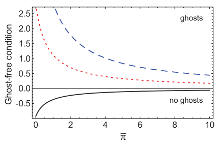
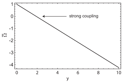
Figure 1: In the left panel, we plot the quantity $\frac{Z^{2}}{2\bar{\Omega}}+\frac{Z\bar{\Omega}_{,\pi}}{\bar{\Omega}}-\frac{9\bar{\pi}^{\prime\prime}}{8m_{6}^{2}}$ which appears in the ghost-free condition (35) for $\Omega=1+3\pi/2$ and $\Lambda=M_{6}^{4}$. The three curves correspond to the three roots of the cubic equation (18) in $\bar{\pi}^{\prime}/m_{6}$. The ghost-free condition requires $\frac{Z^{2}}{2\bar{\Omega}}+\frac{Z\bar{\Omega}_{,\pi}}{\bar{\Omega}}-\frac{9\bar{\pi}^{\prime\prime}}{8m_{6}^{2}}<0$, hence only the black (solid) curve is free of ghost instabilities. In the right panel, we plot $\bar{\Omega}(y)$ for the ghost-free case. Since $\bar{\Omega}$ vanishes at finite $y$, corresponding to strong coupling, this solution is unphysical. We have found similar results for all positive values of $\Lambda$ and functional forms of $\Omega$ that we have tried.

For negative tension, $\Lambda<0$, on the other hand, it is possible to find suitable $\Omega(\pi)$ that satisfy the ghost-free condition and are well-defined for all $y>0$. Figure 2 illustrates this for $\Omega=1+3\pi/2$ and $\Lambda=-M_{6}^{4}$. However, this is only the case for sufficiently small values of the tension, $|\Lambda|\lesssim M_{6}^{4}$. For large values $|\Lambda|\gg M_{6}^{4}$, either the ghost-free condition cannot be satisfied or $\Omega(y)$ is ill-behaved. The existence of non-singular, ghost-free degravitated solutions, albeit with negative tension, is certainly a welcome feature of our $5D$ covariant framework. That said, these solutions do not connect to the parent $6D$ cascading framework, where the deficit angle solution requires a positive tension source.

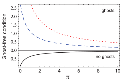
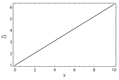
Figure 2: Same as Fig. 1, except that $\Omega=1+3\pi/2$ and $\Lambda=-M_{6}^{4}$. From the right panel, we see that $\bar{\Omega}(y)$ corresponding to the ghost-free branch is everywhere positive, hence this solution is physically viable.

Coming back to (34), there are other requirements that our degravitated solutions must satisfy. To avoid gradient instabilities in the extra dimension, the coefficient of $\zeta^{\prime 2}$ must be negative, which is automatically true since $\Omega>0$. Furthermore, from the ratio of the $\zeta^{\prime 2}$ and $(\partial\zeta)^{2}$ terms we can infer the sound speed of propagation in the bulk:

$$c_{s}^{2}=\frac{-\frac{Z^{2}}{\bar{\Omega}}}{\frac{Z^{2}}{2\bar{\Omega}}+\frac{Z\bar{\Omega}_{,\pi}}{\bar{\Omega}}-\frac{9\bar{\pi}^{\prime\prime}}{8m_{6}^{2}}}\ ,$$ (36)

which is of course manifestly positive once (35) is satisfied. Using this we can determine whether the propagation of perturbations is sub- or super-luminal. For the ghost-free example $\Omega=1+3\pi/2$ and $\Lambda=-M_{6}^{4}$ shown in Fig. 2, $c_{s}^{2}$ is sub-luminal everywhere.

Finally, the coefficient of $(\partial\zeta)^{2}$ on the brane must be negative, in order to avoid ghost instabilities:

$$Z_{0}^{2}-\frac{9m_{5}\bar{\pi}^{\prime}_{0}}{2m_{6}^{2}}\left(1-\frac{9\bar{\pi}^{\prime 2}_{0}}{4m_{6}^{2}Z_{0}}\right)^{-1}<0\ .$$ (37)

With $m_{5}\geq m_{6}$, for instance, this condition is satisfied for the negative-tension example of Fig. 2. As a check, we can compare this ghost-free condition with the stability bound (1) obtained both in the decoupling limit de Rham et al. (2008a) and in the full $6D$ cascading framework de Rham et al. (2010). In the decoupling limit with $\Omega=1-3\pi/2$, where we expect agreement with the cascading results, (37) indeed reduces to $\Lambda>2m_{6}^{2}M_{4}^{2}/3$.

Note that the absence of ghosts on the brane can always be achieved by adding a suitably-large kinetic term for $\pi$ on the brane, thereby modifying (37) to a trivial condition. This intrinsic kinetic term would not affect the background solution nor the bulk perturbation analysis. In this sense, the bulk ghost-free condition (35) is a more robust constraint on the theory.

V Conclusions

Cascading gravity is an interesting approach to understanding dark energy as a manifestation of the presence of large extra dimensions. Unlike previous attempts, such as the DGP model, the propagators in cascading gravity are free of divergences, and the model has been found to be perturbatively ghost-free. Moreover, cascading gravity offers a promising arena for realizing degravitation: both in the codimension-2  de Rham et al. (2008a) and codimension-3 de Rham et al. (2009) cases, at least for small brane tension, the bulk geometry has been shown to be non-singular and asymptotically-flat, while the induced $4D$ geometry is flat.

In this paper, we have studied a recently-proposed effective $5D$ action of cascading gravity in an attempt to obtain flat brane solutions. Our analysis has uncovered an intringuing screening mechanism that can shield bulk gravity from a large tension on the brane, resulting in a small brane extrinsic curvature. The brane remains flat for arbitrarily large tension, while the bulk is non-singular. Although this model offers an attractive mechanism to generalize extra-dimension dark energy models to higher codimensions without any fine-tuning, the stability analysis imposes stringent constraints. The bulk solution is perturbatively unstable for positive brane tension, while it is possible to find stable solutions for sufficiently small negative brane tension.

Our model agrees with earlier work in the weak-field limit, hence we do not contradict results that cascading gravity is indeed ghost-free. It does, however, raise the interesting question — is there a fundamental difference between a theory with large extra dimensions and an effective $4D$ scalar-tensor theory of gravity? A complete answer to this question demands a more detailed analysis, which we leave to future work.

To improve stability, we are currently investigating the impact of including higher-order galileon terms for $\pi$ in the bulk, generalizing the results of Nicolis et al. (2009) to $5D$. Preliminary results show that these higher-order terms still allow for flat brane solutions, while greatly alleviating the stability issues. In particular, ghost-free solutions are now possible with positive tension. However, demanding that gravity on the brane is approximately $4D$ on sufficiently large scales appears to impose an upper bound on the brane tension. The results of this ongoing analysis will be presented in detail elsewhere.

Appendix: Alternative analysis of scalar perturbations

In this appendix we present an alternative derivation of the bulk $\zeta$-action in (34), by performing the stability analysis in the Einstein frame: $g_{MN}^{\rm E}=\Omega^{2/3}g_{MN}^{\rm J}$. We define a warp factor $a_{E}(y)=\Omega^{1/3}(y)$ and a rescaled coordinate ${\rm d}y_{\rm E}=\Omega^{1/3}{\rm d}y$. Removing the subscripts “$E$” for simplicity, the bulk metric in Einstein frame is

$${\rm d}s^{2}_{\rm bulk}=a^{2}(y)(-{\rm d}\tau^{2}+{\rm d}\vec{x}^{2})+{\rm d}y^{2}\ .$$ (A1)

The Einstein frame bulk action is given by

$$S_{\rm bulk} = \frac{M_{5}^{3}}{2}\int_{\rm bulk}{\rm d}^{5}x\sqrt{-g_{5}}\left[R_{5}-\frac{4}{\Omega}\left(\frac{\Omega_{,\pi}^{2}}{\Omega}-\frac{2\Omega_{,\pi\pi}}{3}\right)(\partial\pi)^{2}+\frac{8\Omega_{,\pi}}{3\Omega}(\Box_{5}\pi)\right]$$ (A2)

$$-\ \frac{27M_{5}^{3}}{32m_{6}^{2}}\int_{\rm bulk}{\rm d}^{5}x\sqrt{-g_{5}}(\partial\pi)^{2}\left[\frac{1}{\Omega^{1/3}}\Box_{5}\pi-\frac{\Omega_{,\pi}}{\Omega^{4/3}}(\partial\pi)^{2}\right]\ .$$

Varying with respect to the metric yields the Einstein equations, $M_{5}^{3}G_{MN}=T_{MN}^{\pi}$, where the $\pi$ stress-energy tensor, $T_{MN}^{\pi}=-(2/\sqrt{-g_{5}})\delta S_{\pi}/\delta g^{MN}$, is given by,

$$T_{MN}^{\pi} = \frac{2M_{5}^{3}}{3}\frac{\Omega_{,\pi}^{2}}{\Omega^{2}}\Big{[}2\partial_{M}\pi\partial_{N}\pi-g_{MN}(\partial\pi)^{2}\Big{]}+\ \frac{9M_{5}^{3}}{16m_{6}^{2}}\frac{\Omega_{,\pi}}{\Omega^{4/3}}\Big{[}g_{MN}(\partial\pi)^{4}-4\partial_{M}\pi\partial_{N}\pi(\partial\pi)^{2}\Big{]}$$ (A3)

$$-\ \frac{27M_{5}^{3}}{16m_{6}^{2}}\Omega^{-1/3}\Bigg{[}\partial_{(M}(\partial\pi)^{2}\partial_{N)}\pi-\frac{1}{2}g_{MN}\partial_{K}(\partial\pi)^{2}\partial^{K}\pi-\partial_{M}\pi\partial_{N}\pi\Box_{5}\pi$$

$$+\ \frac{\Omega_{,\pi}}{3\Omega}\partial_{M}\pi\partial_{N}\pi(\partial\pi)^{2}\Bigg{]}\ .$$

For the metric (A1) with $\pi\equiv\pi(y)$, the $(5,5)$ and $(\mu,\nu)$ components of the Einstein equations give us the following background evolution equations,

$$6H^{2} = \rho\ ,$$ (A4)

$$3H^{\prime} = -(\rho+p)\ ,$$ (A5)

where

$$\rho = \frac{2}{3}\left[\left(\frac{\Omega_{,\pi}}{\Omega}\right)^{2}\pi^{\prime 2}-\frac{27}{8m_{6}^{2}}\Omega^{-1/3}\left(\frac{\Omega_{,\pi}}{\Omega}\pi^{\prime 4}-3H\pi^{\prime 3}\right)\right]\ ,$$ (A6)

$$p = \frac{2}{3}\left[\left(\frac{\Omega_{,\pi}}{\Omega}\right)^{2}\pi^{\prime 2}-\frac{27}{32m_{6}^{2}}\Omega^{-1/3}\left(\frac{\Omega_{,\pi}}{\Omega}\pi^{\prime 4}+3\pi^{\prime 2}\pi^{\prime\prime}\right)\right]\ .$$ (A7)

Here $H=a^{\prime}/a$ is the $5D$ Hubble parameter, with $y$ playing the role of a “time” variable.

To study scalar perturbations, we use ADM coordinates (23) and choose comoving gauge: $q_{\mu\nu}=a^{2}(y)e^{2\zeta(x^{\mu},y)}\eta_{\mu\nu}$ and $\pi=\pi(y)$. In this gauge we cannot assume that the brane is at fixed position, but this is of no consequence here as we focus solely on bulk perturbations. The action (A2) can be rewritten using ADM variables as

$$S_{\rm bulk}=S_{g}+S_{\pi}\,,$$ (A8)

with

$$S_{g} = \frac{M_{5}^{3}}{2}\int_{\rm bulk}{\rm d}^{5}x\sqrt{-q}\left[NR_{4}+\frac{1}{N}\left(E^{2}-E_{\mu\nu}E^{\mu\nu}\right)\right]\ ,$$

$$S_{\pi} = \frac{M_{5}^{3}}{2}\int_{\rm bulk}{\rm d}^{5}x\sqrt{-q}N\left[-\frac{4}{3}\left(\frac{\Omega_{,\pi}}{\Omega}\right)^{2}\frac{\pi^{\prime 2}}{N^{2}}\right]$$ (A9)

$$- \frac{27M_{5}^{3}}{32m_{6}^{2}}\int_{\rm bulk}{\rm d}^{5}x\sqrt{-q}N\frac{\pi^{\prime 2}}{N^{2}}\left[\Omega^{-1/3}\left(\frac{2}{3}\frac{\pi^{\prime}}{N}K-\frac{8}{9}\frac{\Omega_{,\pi}}{\Omega}\frac{\pi^{\prime 2}}{N^{2}}\right)\right]\ ,$$

where $E_{\mu\nu}=(q_{\mu\nu}^{\prime}-D_{\mu}N_{\nu}-D_{\nu}N_{\mu})/2=NK_{\mu\nu}$.

Expanded to second order in the perturbations, $\delta N=N-1$ and $\delta{E^{\alpha}}_{\alpha}={E^{\alpha}}_{\alpha}-4H$, the scalar field action reduces to

$$S_{\pi} = \frac{M_{5}^{3}}{2}\int_{\rm bulk}{\rm d}^{5}x\sqrt{-q}N\Bigg{[}3H^{\prime}\frac{1}{N^{2}}+3(4H^{2}+H^{\prime})+\frac{1}{2}M^{4}(y)\delta N^{2}-\hat{M}^{3}(y)\delta{E^{\alpha}}_{\alpha}\delta N\Bigg{]}\ ,$$

where

$$M^{4}(y) = -\frac{27}{8m_{6}^{2}}\Omega^{-1/3}\left(-\frac{11}{3}\frac{\Omega_{,\pi}}{\Omega}\pi^{\prime 4}+\pi^{\prime 2}\pi^{\prime\prime}+12H\pi^{\prime 3}\right)\ ,$$ (A11)

$$\hat{M}^{3}(y) = -\frac{27}{8m_{6}^{2}}\Omega^{-1/3}\pi^{\prime 3}\ .$$ (A12)

Varying the complete bulk action with respect to $N^{\mu}$ and $N$ gives us the momentum and Hamiltonian constraint equations,

$$D_{\alpha}\left[\frac{2}{N}(E{\delta^{\alpha}}_{\beta}-{E^{\alpha}}_{\beta})-\hat{M}^{3}\delta N{\delta^{\alpha}}_{\beta}\right]=0\ ,$$ (A13)

$$R_{4}-\frac{1}{N^{2}}(E^{2}-E_{\mu\nu}E^{\mu\nu})-\frac{3}{N^{2}}H^{\prime}+3(4H^{2}+H^{\prime})+M^{4}\delta N-\hat{M}^{3}\delta{E^{\alpha}}_{\alpha}=0\ .$$ (A14)

For scalar perturbations, $q_{\mu\nu}=a^{2}(y)e^{2\zeta(x^{\mu},y)}\eta_{\mu\nu}$ and $N_{\mu}\equiv\partial_{\mu}\beta$, the first-order solutions to (A13) and (A14) are given by

$$\delta N = \frac{6\zeta^{\prime}}{6H+\hat{M}^{3}}\ ,$$ (A15)

$$\Box_{4}\beta = \frac{6}{6H+\hat{M}^{3}}\frac{1}{a^{2}}\partial^{2}\zeta+\frac{-36H^{\prime}+48H\hat{M}^{3}+4\hat{M}^{6}-6M^{4}}{(6H+\hat{M}^{3})^{2}}\zeta^{\prime}\ .$$ (A16)

As usual, we only need to solve the constraint equations at first-order in the perturbations to obtain the quadratic Lagrangian for $\zeta$, since the second-order terms will multiply the unperturbed constraint equations, which vanish Maldacena (2003). Also note that here $\Box_{4}\beta=q^{\mu\nu}D_{\mu}D_{\nu}\beta$ whereas $\partial^{2}\zeta=\eta^{\mu\nu}\partial_{\mu}\partial_{\nu}\zeta$.

The quadratic action for $\zeta$ is obtained by plugging back the solutions (A15) and (A16) into the original action (A8), (A9). We find that all of the $\Box_{4}\beta$ terms add up to a total derivative, hence the final Einstein frame $\zeta-$action is

$$S_{\zeta} = \frac{M_{5}^{3}}{2}\int_{\rm bulk}{\rm d}^{5}x\ a^{4}\left[A(y)\zeta^{\prime 2}+B(y)\frac{1}{a^{2}}(\partial\zeta)^{2}\right]\ ,$$ (A17)

where

$$A(y) = \frac{6(18H^{\prime}-24H\hat{M}^{3}-2\hat{M}^{6}+3M^{4})}{(6H+\hat{M}^{3})^{2}}\ ,$$ (A18)

$$B(y) = \frac{6(18H^{\prime}+6H\hat{M}^{3}+\hat{M}^{6}+3\partial_{y}\hat{M}^{3})}{(6H+\hat{M}^{3})^{2}}\ ,$$ (A19)

and $(\partial\zeta)^{2}=\eta^{\mu\nu}\partial_{\mu}\zeta\partial_{\nu}\zeta$.

We can transform the action (A17) back to the Jordan frame by using the transformations between Einstein frame variables (now denoted with a subscript “$E$”) and Jordan frame variables: $a_{\rm E}=\Omega^{1/3}$, ${\rm d}y_{\rm E}=\Omega^{1/3}{\rm d}y$, and $\zeta_{\rm E}=\zeta$. The result is

$$S_{\zeta}^{\rm Jordan} = \frac{M_{5}^{3}}{2}\int_{\rm bulk}{\rm d}^{5}x\left[-12\Omega\zeta^{\prime 2}+\frac{12\Omega^{2}}{Z^{2}}\left(\frac{Z^{2}}{2\Omega}+\frac{Z\Omega_{,\pi}}{\Omega}-\frac{9\pi^{\prime\prime}}{8m_{6}^{2}}\right)(\partial\zeta)^{2}\right]\ ,$$ (A20)

which matches with the bulk Jordan frame action in (34).

References

- Lukas et al. (1999) A. Lukas, B. A. Ovrut, K. S. Stelle, and D. Waldram, Phys. Rev. D59, 086001 (1999), eprint hep-th/9803235.
- Arkani-Hamed et al. (1998) N. Arkani-Hamed, S. Dimopoulos, and G. R. Dvali, Phys. Lett. B429, 263 (1998), eprint hep-ph/9803315.
- Antoniadis et al. (1998) I. Antoniadis, N. Arkani-Hamed, S. Dimopoulos, and G. R. Dvali, Phys. Lett. B436, 257 (1998), eprint hep-ph/9804398.
- Randall and Sundrum (1999a) L. Randall and R. Sundrum, Phys. Rev. Lett. 83, 3370 (1999a), eprint hep-ph/9905221.
- Randall and Sundrum (1999b) L. Randall and R. Sundrum, Phys. Rev. Lett. 83, 4690 (1999b), eprint hep-th/9906064.
- Dvali et al. (2000) G. R. Dvali, G. Gabadadze, and M. Porrati, Phys. Lett. B485, 208 (2000), eprint hep-th/0005016.
- Rydbeck et al. (2007) S. Rydbeck, M. Fairbairn, and A. Goobar, JCAP 0705, 003 (2007), eprint astro-ph/0701495.
- Fang et al. (2008) W. Fang et al., Phys. Rev. D78, 103509 (2008), eprint 0808.2208.
- Lombriser et al. (2009) L. Lombriser, W. Hu, W. Fang, and U. Seljak, Phys. Rev. D80, 063536 (2009), eprint 0905.1112.
- Guo et al. (2006) Z.-K. Guo, Z.-H. Zhu, J. S. Alcaniz, and Y.-Z. Zhang, Astrophys. J. 646, 1 (2006), eprint astro-ph/0603632.
- Nicolis and Rattazzi (2004) A. Nicolis and R. Rattazzi, JHEP 06, 059 (2004), eprint hep-th/0404159.
- Koyama (2005) K. Koyama, Phys. Rev. D72, 123511 (2005), eprint hep-th/0503191.
- Gorbunov et al. (2006) D. Gorbunov, K. Koyama, and S. Sibiryakov, Phys. Rev. D73, 044016 (2006), eprint hep-th/0512097.
- Charmousis et al. (2006) C. Charmousis, R. Gregory, N. Kaloper, and A. Padilla, JHEP 10, 066 (2006), eprint hep-th/0604086.
- Dvali et al. (2007a) G. Dvali, G. Gabadadze, O. Pujolas, and R. Rahman, Phys. Rev. D75, 124013 (2007a), eprint hep-th/0612016.
- Gregory et al. (2007) R. Gregory, N. Kaloper, R. C. Myers, and A. Padilla, JHEP 10, 069 (2007), eprint 0707.2666.
- Rubakov and Shaposhnikov (1983) V. A. Rubakov and M. E. Shaposhnikov, Phys. Lett. B125, 139 (1983).
- Weinberg (1989) S. Weinberg, Rev. Mod. Phys. 61, 1 (1989).
- Gibbons et al. (2001) G. W. Gibbons, R. Kallosh, and A. D. Linde, JHEP 01, 022 (2001), eprint hep-th/0011225.
- Dvali et al. (2003) G. Dvali, G. Gabadadze, and M. Shifman, Phys. Rev. D67, 044020 (2003), eprint hep-th/0202174.
- Arkani-Hamed et al. (2002) N. Arkani-Hamed, S. Dimopoulos, G. Dvali, and G. Gabadadze (2002), eprint hep-th/0209227.
- Dvali et al. (2007b) G. Dvali, S. Hofmann, and J. Khoury, Phys. Rev. D76, 084006 (2007b), eprint hep-th/0703027.
- Dvali and Gabadadze (2001) G. R. Dvali and G. Gabadadze, Phys. Rev. D63, 065007 (2001), eprint hep-th/0008054.
- Dubovsky and Rubakov (2003) S. L. Dubovsky and V. A. Rubakov, Phys. Rev. D67, 104014 (2003), eprint hep-th/0212222.
- Gabadadze and Shifman (2004) G. Gabadadze and M. Shifman, Phys. Rev. D69, 124032 (2004), eprint hep-th/0312289.
- de Rham et al. (2008a) C. de Rham et al., Phys. Rev. Lett. 100, 251603 (2008a), eprint 0711.2072.
- de Rham et al. (2008b) C. de Rham, S. Hofmann, J. Khoury, and A. J. Tolley, JCAP 0802, 011 (2008b), eprint 0712.2821.
- Corradini et al. (2008a) O. Corradini, K. Koyama, and G. Tasinato, Phys. Rev. D77, 084006 (2008a), eprint 0712.0385.
- Corradini et al. (2008b) O. Corradini, K. Koyama, and G. Tasinato, Phys. Rev. D78, 124002 (2008b), eprint 0803.1850.
- de Rham et al. (2009) C. de Rham, J. Khoury, and A. J. Tolley, Phys. Rev. Lett. 103, 161601 (2009), eprint 0907.0473.
- de Rham et al. (2010) C. de Rham, J. Khoury, and A. J. Tolley, Phys. Rev. D81, 124027 (2010), eprint 1002.1075.
- Agarwal et al. (2010) N. Agarwal, R. Bean, J. Khoury, and M. Trodden, Phys. Rev. D81, 084020 (2010), eprint 0912.3798.
- Nicolis et al. (2009) A. Nicolis, R. Rattazzi, and E. Trincherini, Phys. Rev. D79, 064036 (2009), eprint 0811.2197.
- Luty et al. (2003) M. A. Luty, M. Porrati, and R. Rattazzi, JHEP 09, 029 (2003), eprint hep-th/0303116.
- Chow and Khoury (2009) N. Chow and J. Khoury, Phys. Rev. D80, 024037 (2009), eprint 0905.1325.
- Deffayet et al. (2009) C. Deffayet, G. Esposito-Farese, and A. Vikman, Phys. Rev. D79, 084003 (2009), eprint 0901.1314.
- Silva and Koyama (2009) F. P. Silva and K. Koyama, Phys. Rev. D80, 121301 (2009), eprint 0909.4538.
- De Felice and Tsujikawa (2010) A. De Felice and S. Tsujikawa, Phys. Rev. Lett. 105, 111301 (2010), eprint 1007.2700.
- Mota et al. (2010) D. F. Mota, M. Sandstad, and T. Zlosnik, JHEP 12, 051 (2010), eprint 1009.6151.
- Kachru et al. (2000) S. Kachru, M. B. Schulz, and E. Silverstein, Phys. Rev. D62, 045021 (2000), eprint hep-th/0001206.
- York (1972) J. York, James W., Phys. Rev. Lett. 28, 1082 (1972).
- Gibbons and Hawking (1977) G. W. Gibbons and S. W. Hawking, Phys. Rev. D15, 2752 (1977).
- Dyer and Hinterbichler (2009) E. Dyer and K. Hinterbichler, JHEP 11, 059 (2009), eprint 0907.1691.
- Nicolis et al. (2010) A. Nicolis, R. Rattazzi, and E. Trincherini, JHEP 05, 095 (2010), eprint 0912.4258.
- Arnowitt et al. (1962) R. L. Arnowitt, S. Deser, and C. W. Misner (1962), eprint gr-qc/0405109.
- Maldacena (2003) J. M. Maldacena, JHEP 05, 013 (2003), eprint astro-ph/0210603.