Spatially Coupled LDPC Codes for Decode-and-Forward in Erasure Relay Channel

Abstract

We consider spatially-coupled protograph-based LDPC codes for the three terminal erasure relay channel. It is observed that BP threshold value, the maximal erasure probability of the channel for which decoding error probability converges to zero, of spatially-coupled codes, in particular spatially-coupled MacKay-Neal code, is close to the theoretical limit for the relay channel. Empirical results suggest that spatially-coupled protograph-based LDPC codes have great potential to achieve theoretical limit of a general relay channel.

I Introduction

Felström and Zigangirov constructed the time-varying periodic Low-Density Parity-Check (LDPC) convolutional codes from LDPC block codes [1]. Surprisingly, the LDPC convolutional codes outperform the constituent underlying LDPC block codes. Recently, Kudekar et al. rigorously proved such decoding performance improvement over binary erasure channels (BEC) and showed that the terminated LDPC convolutional coding increases the belief propagation (BP) threshold up to the maximum a-priori (MAP) threshold of the underlying block code. This phenomenon is called threshold saturation [2]. A protograph of an LDPC convolutional code can be seen that a spatially coupled protograph of the underlying LDPC code, hence Kudekar et al. named this code spatially-coupled protograph-based LDPC code.

Spatially-coupled protograph-based LDPC codes, composed of many identical protographs coupled with their neighboring protographs, have recently attracted much attentions. The threshold saturation phenomenon is observed not only for the BEC, but also for general binary memoryless symmetric (BMS) channels [3]. It is expected that the spatially-coupled protograph-based LDPC codes achieve universally the capacity of the BMS channels under BP decoding. Such universality is not possessed by polar codes [4] or irregular LDPC codes [5]. Depending on the channel, frozen bits need to be optimized for polar codes and degree distributions need to be optimized for irregular LDPC codes. Therefore, it is expected that the spatially-coupled protograph-based LDPC codes are able to be applied to many other problems in communications.

Recently, Kudekar and Kasai showed empirical evidences that the BP threshold value of the spatially-coupled protograph-based LDPC codes is approaching the theoretical limit for a class of channels with memory [6] and the Shannon threshold over multiple access channels [7].

MacKay-Neal (MN) codes [8] are non-systematic two-edge type LDPC codes [9]. The MN codes are conjectured to achieve the capacity of BMS channels under maximum likelihood decoding. Murayama et al. [10] and Tanaka et al. [11] reported the empirical evidence of the conjecture for BSC and AWGN channels, respectively by a non-rigorous statistical mechanics approach known as replica method. Recently, Kasai et al. have shown that spatially-coupled MN codes have the BP thresholds very close to the Shannon limit of the BEC [12].

It is naturally expected that the same phenomenon occurs also for transmission over relay channels. We propose spatially-coupled protograph-based LDPC and MN codes for DF strategy over erasure relay channels. BP decoding of joint use of Tanner graphs is presented, and density evolution analysis gives an empirical evidence that spatially-coupled protograph-based MN codes achieve theoretical limit of the erasure relay channel.

The paper is organized as follows. Section II introduces the erasure relay channel and the DF strategy. Section III defines spatially-coupled protograph-based LDPC and MN codes. Section IV describes the density evolution equations. The numerical results are presented in Section V. The last section will conclude.

II Erasure Relay Channel

II-A Channel Model

We show the erasure relay channel used in this paper in Fig. 1. The relay channel comprises of a sender node $\mathsf{S}$, a destination node $\mathsf{D}$, and a relay node $\mathsf{R}$. For simplicity, interferences between the sender and the relay transmissions are not considered in this paper, therefore we can view the above relay channel as two separate channels. One is an erasure-broadcast channel from $\mathsf{S}$ to $\mathsf{R}$ and $\mathsf{D}$, and the other is a point-to-point erasure channel from $\mathsf{R}$ to $\mathsf{D}$. We denote that the erasure probabilities on the channels from $\mathsf{S}$ to $\mathsf{R}$, from $\mathsf{R}$ to $\mathsf{D}$, and from $\mathsf{S}$ to $\mathsf{D}$ by $\epsilon_{\mbox{\tiny\sf SR}}$, $\epsilon_{\mbox{\tiny\sf RD}}$, and $\epsilon_{\mbox{\tiny\sf SD}}$, respectively. This relay channel can be regarded as wireless communication network from the viewpoint of higher layer [13].

Figure 1: Erasure relay channel.

II-B Capacity of Erasure Relay Channel

Denote the coding rate at $\mathsf{S}$ by $R$.

Theorem 1 (Capacity [13]).

The achievable rate region of the erasure relay channel without interferences at $\mathsf{D}$ is given by:

$$R\leq\min\{(1-\epsilon_{\mbox{\tiny\sf SD}}\epsilon_{\mbox{\tiny\sf SR}}),(1-\epsilon_{\mbox{\tiny\sf SD}})+\beta(1-\epsilon_{\mbox{\tiny\sf RD}})\},$$

where $\beta=1$ if $R<1-\epsilon_{\mbox{\tiny\sf SR}}$ and $\beta=\epsilon_{\mbox{\tiny\sf SR}}$ otherwise. Since the DF strategy is employed, i.e., $R<1-\epsilon_{\mbox{\tiny\sf SR}}$ in this paper, it holds that $\beta=1.$ The region, therefore, becomes

$$R\leq\min\{(1-\epsilon_{\mbox{\tiny\sf SR}}),(1-\epsilon_{\mbox{\tiny\sf SD}})+(1-\epsilon_{\mbox{\tiny\sf RD}})\}.$$ (1)

The dashed lines in Fig. 2 represents the boundary of the region for fixed coding rate $R=0.5$. We will define a code pair used at $\mathsf{S}$ and $\mathsf{R}$ in Section III. In Section IV, we will investigate the achievable region of $(\epsilon_{\mbox{\tiny\sf S}\mbox{\tiny\sf R}},\epsilon_{\mbox{\tiny\sf S}\mbox{\tiny\sf D}})$ for the code pair.

II-C LDPC Coding for DF Strategy

Let $N_{\mbox{\tiny\sf S}}$ and $N_{\mbox{\tiny\sf R}}$ are the lengths of codes used at $\mathsf{S}$ and $\mathsf{R}$, respectively. We denote the codewords sent from $\mathsf{S}$ and $\mathsf{R}$ by $\bm{x}\in\{0,1\}^{N_{\mathsf{S}}}$ and $\bm{x}^{\prime}\in\{0,1\}^{N_{\mathsf{R}}}$, respectively. We denote the received words at $\mathsf{R}$ and $\mathsf{D}$ from $\mathsf{S}$ by $\bm{y}_{\mathsf{R}}\in\{0,1,?\}^{N_{\mathsf{S}}}$, $\bm{y}_{\mathsf{D}}\in\{0,1,?\}^{N_{\mathsf{S}}}$, respectively. We denote the received words at $\mathsf{D}$ from $\mathsf{R}$ by $\bm{y}^{\prime}\in\{0,1,?\}^{N_{\mathsf{R}}}$.

Design of LDPC codes for relay channels with DF strategy was discussed in several papers [14], [15], [16], [17]. The sender $\mathsf{S}$ sends a codeword $\bm{x}$ encoded by an LDPC code. The relay $\mathsf{R}$ decodes $\bm{x}$. We assume the decoding error probability is arbitrary small. This is realized by capacity approaching codes and due to the DF strategy assumption $R<1-\epsilon_{\mbox{\tiny\sf SR}}$. Then $\mathsf{R}$ generates $\bm{x}^{\prime}$ from $\bm{x}$ using another LDPC code. $\bm{x}^{\prime}$ is transmitted to $\mathsf{D}$. $\mathsf{D}$ decodes the codeword $\bm{x}$ from $\bm{y}_{\mathsf{D}}$ and $\bm{y}^{\prime}$. This decoding process at $\mathsf{D}$ is performed by joint use of Tanner graphs of the two LDPC codes.

III Spatially-Coupled Protograph-based Codes

In this section, we define spatially-coupled protograph-based LDPC and MN codes, respectively.

III-A Protograph-based Codes

Protograph-based codes are defined by the Tanner graphs lifted from relatively small graphs called protographs [18][19]. Protographs are defined by non-negative integer matrices called base-matrices [20]. Let us assume we are given a base-matrix $\bm{{\rm B}}\in(\mathbb{Z}^{+})^{m_{p}\times n_{p}}$. The parity-check matrix is obtained by replacing each entry of $\bm{{\rm B}}(i,j)$ with a $q\times q$ binary matrix which is the sum of $\bm{{\rm B}}(i,j)$-times randomly chosen $q\times q$ permutation matrices over $\mathrm{GF}(2)$. Note that the zero entry of $\bm{{\rm B}}$ is replaced with a $q\times q$ all-zero binary matrix. This lifting process of matrices keeps the weight of columns and rows the same.

III-B Spatially-Coupled Protograph-based Codes

We define a spatially-coupled base-matrix $\bm{{\rm B}}_{[0,L-1]}$ from a given base-matrix $\bm{{\rm B}}\in(\mathbb{Z}^{+})^{m_{p}\times n_{p}}$. Let $L$ be a non-negative integer, which is referred to as coupling number. We define $\bm{{\rm B}}_{[0,L-1]}$ as follows.

$$\bm{{\rm B}}_{[0,L-1]} =\begin{bmatrix}\bm{{\rm B}}_{0}&\\ \vdots&\ddots&\\ \bm{{\rm B}}_{d}&&\bm{{\rm B}}_{0}\\ &\ddots&\vdots\\ &&\bm{{\rm B}}_{d}\end{bmatrix}\in(\mathbb{Z}^{+})^{m_{p}(L+d)\times n_{p}L},$$

where $\bm{{\rm B}}_{0},\dotsc,\bm{{\rm B}}_{d}\in(\mathbb{Z}^{+})^{m_{p}\times n_{p}}$ are non-negative integer matrices chosen so that

$$\sum_{i=0}^{d}\bm{{\rm B}}_{i}=\bm{{\rm B}}\in(\mathbb{Z}^{+})^{m_{p}\times n_{p}},$$

for some $d$. These matrices are referred to as spreading base-matrices.

III-C Spatially-Coupled Protograph-based ($l,r,L$)-regular LDPC Codes

We define the base-matrix of protograph-based ($l$,$r$)-regular LDPC codes as

$$\bm{{\rm B}}^{(l,r)} :=[l,\cdots,l]\in(\mathbb{Z}^{+})^{1\times k},$$

where we assumed $r=kl$ for some integer $k$, for simplicity. Spatially-coupled protograph-based ($l,r,L$)-regular LDPC codes are defined as protograph-based codes defined by spreading base-matrices

$$\bm{{\rm B}}_{i}^{(l,r)}=[1,\dotsc,1]\in(\mathbb{Z}^{+})^{1\times k}\text{ for }0\leq i\leq l-1.$$

The design rate $R^{(l,r,L)}$ of the spatially-coupled protograph-based ($l,r,L$)-regular LDPC codes is given by

$$R^{(l,r,L)}=1-\frac{(L+l-1)}{Lk}=R^{(l,r)}-\frac{(1-R^{(l,r)})(l-1)}{L}.$$ (2)

$R^{(l,r)}=1-1/k$ is the design rate of the underlying code. $R^{(l,r,L)}$ converges to $R^{(l,r)}$ as increasing $L$ with gap $O(1/L)$. We use bits corresponding to the leftmost column of $\bm{{\rm B}}^{(l,r)}$ and $\bm{{\rm B}}_{i}^{(l,r)}$ for $i=0,\dotsc,l-1$ as information bits.

III-D Spatially-Coupled Protograph-based ($l,r,g,L$)-MN Codes

We define the base-matrix of protograph-based ($l,r,g$)-MN codes as

$$\bm{{\rm B}}^{{\mathrm{MN}}(l,r,g)} :=\begin{bmatrix}r&1&\cdots&1\\ \vdots&\vdots&\ddots&\vdots\\ r&1&\cdots&1\end{bmatrix}\in(\mathbb{Z}^{+})^{g\times g+1},$$

where we assumed $l=gr$, for simplicity. MN codes have punctured nodes, therefore the bits corresponding to the leftmost column of $\bm{{\rm B}}^{{\mathrm{MN}}(l,r,g)}$ are punctured.

Spatially-coupled protograph-based ($l,r,g,L$)-MN codes are defined as protograph-based codes defined by spreading base-matrices $\bm{{\rm B}}_{i}^{{\mathrm{MN}}(l,r,g)}$ for $i=0,\dotsc,g-1$ as follows

$$\bm{{\rm B}}_{i}^{{\mathrm{MN}}(l,r,g)} =\begin{bmatrix}\bm{0}_{i-1\times g+1}\\ \bm{{\rm b}}_{i}\\ \bm{0}_{g-i\times g+1}\end{bmatrix},$$

$$\bm{{\rm b}}_{i} =[r-1,\bm{0}_{1\times g-i},\bm{1}_{i}]\text{ for }1\leq i\leq g-1,$$

$$\bm{{\rm B}}_{0}^{{\mathrm{MN}}(l,r,g)} =\bm{{\rm B}}^{{\mathrm{MN}}(l,r,g)}-\sum_{i=1}^{g-1}\bm{{\rm B}}_{i}^{{\mathrm{MN}}(l,r,g)},$$

where $\bm{0}_{a\times b}$ represents an $a\times b$ all-zero matrix and $\bm{1}_{i}$ represents an all-one row vector of length $i$.

The design rate $R^{{\mathrm{MN}}(l,r,g,L)}$ of the spatially-coupled protograph-based ($l,r,g,L$)-MN codes is given by

$$R^{{\mathrm{MN}}(l,r,g,L)} =1-\frac{(g+1)L-(gL+g-1)}{L(g+1)-L}$$

$$=R^{{\mathrm{MN}}(l,r,g)}-\frac{1-R^{{\mathrm{MN}}(l,r,g)}}{L}.$$ (3)

$R^{{\mathrm{MN}}(l,r,g)}=1/g$ is the design rate of the underlying code. $R^{{\mathrm{MN}}(l,r,g,L)}$ converges to $R^{{\mathrm{MN}}(l,r,g)}$ as increasing $L$ with gap $O(1/L)$.

We use bits corresponding to the leftmost column of $\bm{{\rm B}}^{{\mathrm{MN}}(l,r,g)}$ and $\bm{{\rm B}}_{i}^{{\mathrm{MN}}(l,r,g)}$ for $i=0,\dotsc,g-1$ as information bits.

III-E Relay Channel Coding via Spatially-Coupled Protograph-based Codes

As explained in Section II-C, we use two LDPC codes for coding at $\mathsf{S}$ and $\mathsf{R}$. We propose a relay channel coding scheme via spatially-coupled protograph-based codes in the following way.

The sender $\mathsf{S}$ encodes the information bits into $\bm{x}$ with a spatially-coupled ($l,r,L$)-regular LDPC (resp. ($l,r,g,L$)-MN) code defined by a base-matrix $\bm{{\rm B}}^{(l,r)}_{[0,L-1]}$ (resp. $\bm{{\rm B}}^{{\mathrm{MN}}(l,r,g)}_{[0,L-1]}$). The relay $\mathsf{R}$ decodes $\bm{x}$ from $\bm{y}_{\mathsf{R}}$ and encodes the information bits into ${\bm{x}}^{\prime}$ with another spatially-coupled ($l,r,L$)-regular LDPC (resp. ($l,r,g,L$)-MN) code defined by the same base-matrix $\bm{{\rm B}}^{(l,r)}_{[0,L-1]}$ (resp. $\bm{{\rm B}}^{{\mathrm{MN}}(l,r,g)}_{[0,L-1]}$).

The destination $\mathsf{D}$ decodes ${\bm{x}}$ from ${\bm{y}}_{\mathsf{D}}$ and ${\bm{y}}^{\prime}$ by BP decoding. The BP decoding algorithm is performed on a Tanner graph which represents the two codes. The joint Tanner graph is obtained by connecting information variable nodes in the two codes with check nodes of degree 2. For example, the joint protograph of spatially-coupled (3,6,24)-regular LDPC and (4,2,2,12)-MN codes are depicted in Figs. 4 and  7, respectively.

IV Density Evolution Analysis

The BP decoder [21] iteratively exchanges messages $\in\{0,1,?\}$ between variable nodes and check nodes in the Tanner graphs. For transmissions over the BEC, the density evolution allows us to predict the message erasure probability at each iteration round.

Let us assume we are given two protograph-based codes defined by a spatially-coupled base-matrix $\bm{{\rm B}}$. We refer to the edges in the Tanner graph corresponding to the base-matrix entry $\bm{{\rm B}}(i,j)$ as edges at section $(i,j)$. Let $y^{(\ell)}_{i,j}$ denote the probability that the messages from check nodes to variable nodes along the edges at section $(i,j)$ are “$?$” at iteration $\ell$. Similarly, we define $x^{(\ell)}_{i,j}$ as the probability that the messages from variable nodes to check nodes along the edges at section $(i,j)$ are “$?$” at iteration $\ell$. The messages at the 0-th round are initialized with channel outputs. It follows that $x^{(0)}_{i,j}=\epsilon_{j}$, where $\epsilon_{j}$ is defined by $\epsilon_{j}=\epsilon_{\mbox{\tiny\sf SD}}$ (reps. $\epsilon_{\mbox{\tiny\sf RD}}$) if the bits are transmitted by $\mathsf{S}$ (resp. $\mathsf{R}$) and corresponding to the $j$-th column of the base-matrix entry $\bm{{\rm B}}$ are not punctured, and $\epsilon_{j}=1$ otherwise.

A message sent from a check node is “$?$” if and only if at least one of the incoming messages are “$?$”. Consequently, we have

$$y^{(\ell)}_{i,j}=1-(1-x^{(\ell-1)}_{i,j})^{(\bm{{\rm B}}(i,j)-1)}\prod_{j^{\prime}\neq j}(1-x^{(\ell-1)}_{i,j^{\prime}})^{\bm{{\rm B}}(i,j^{\prime})},$$

for $(i,j)$ such that $\bm{{\rm B}}(i,j)\neq 0$.

A message sent from a variable node is “$?$” if all the incoming messages and the message from the channel are “$?$”. Consequently, we have

$$x^{(\ell)}_{i,j}=\epsilon_{j}(y^{(\ell)}_{i,j})^{(\bm{{\rm B}}(i,j)-1)}\prod_{i^{\prime}\neq i}(y^{(\ell)}_{i^{\prime},j})^{\bm{{\rm B}}(i^{\prime},j)},$$

for $(i,j)$ such that $\bm{{\rm B}}(i,j)\neq 0$.

The channel erasure probability pair ($\epsilon_{\mbox{\tiny\sf RD}}$, $\epsilon_{\mbox{\tiny\sf SD}}$) is said to be achievable by the protograph-based codes if $\lim_{\ell\to\infty}x^{(\ell)}_{i,j}=0$ for all $i,j$ such that $\bm{{\rm B}}(i,j)\neq 0$.

V Numerical Results

In this section, we evaluate the achievable ($\epsilon_{\mbox{\tiny\sf RD}}$, $\epsilon_{\mbox{\tiny\sf SD}}$) region, referred to as achievable erasure probability region, for LDPC codes and spatially-coupled protograph-based LDPC and MN codes. We choose $L=128$ so that the difference between $R^{{\mathrm{MN}}(l,r,g,L)}$ and 0.5 is less than 0.01.

V-A Regular LDPC Codes

The joint base matrix of the joint (3,6)-regular LDPC code at $\mathsf{D}$ is given as

$$\bm{{\rm B}}=\begin{bmatrix}3&3&0&0\\ 0&0&3&3\\ 1&0&1&0\\ \end{bmatrix}.$$ (4)

The 2 leftmost columns and the other columns correspond $\bm{x}$ and $\bm{x}^{\prime}$, respectively. Therefore $\epsilon_{j}=\epsilon_{\mbox{\tiny\sf SD}}$ for $j=0~{}\text{and}~{}1$, and $\epsilon_{j^{\prime}}=\epsilon_{\mbox{\tiny\sf SD}}$ for $j^{\prime}=2~{}\text{and}~{}3$. Note that the indices of matrices start from 0. We compute achievable erasure probability region using density evolution with $\bm{{\rm B}}$ as shown in Eq. (4).

Figure 2 shows the achievable erasure probability region of (3,6)-regular LDPC codes of rate 0.5 at $\mathsf{S}$ and $\mathsf{R}$. The vertical axis represents $\epsilon_{\mbox{\tiny\sf SD}}$ and the horizontal axis represents $\epsilon_{\mbox{\tiny\sf RD}}$. The black dashed line represents the theoretical limit Eq. (1) for rate 0.5. It can be seen that there is a large gap in the slope region for $0.5<\epsilon_{\mbox{\tiny\sf RD}}<1$, $0.5<\epsilon_{\mbox{\tiny\sf SD}}<1$.

When $\epsilon_{\mbox{\tiny\sf RD}}=1$, $\bm{y}^{\prime}$ is all erased, $\mathsf{D}$ needs to decode $\bm{x}$ only from $\bm{y}_{\mathsf{D}}$. Hence, the achievable $\epsilon_{\mbox{\tiny\sf SD}}$ when $\epsilon_{\mbox{\tiny\sf RD}}=1$ is equal to the BP threshold of the (3,6)-regular LDPC code 0.4294.

Figure 2: Achievable erasure probability region of (3,6)-regular LDPC codes at $\mathsf{S}$ and $\mathsf{R}$. The black dashed line represents the theoretical limit Eq. (1) for rate 0.5. It can be seen that there is a large gap in the slope region for $0.5<\epsilon_{\mbox{\tiny\sf RD}}<1$, $0.5<\epsilon_{\mbox{\tiny\sf SD}}<1$.

V-B Split-extended LDPC codes [17]

Recently a split-extension technique for LDPC coding over the Gaussian relay channels has been developed by Savin [17]. The performance over the BEC has not been known, therefore we evaluate by using achievable erasure probability region for comparison purpose.

Split-extension technique splits the check node of the protograph to two or more check nodes with variable node of degree 2 in order to generate extra parity bits ${\bm{x}}^{\prime}$ sent from the $\mathsf{R}$ toward the $\mathsf{D}$. When generated variable nodes of degree 2 are punctured, splitted protograph is identical to the original protograph. Hence $\mathsf{R}$ sends bits corresponding to the variable nodes of degree 2 to the $\mathsf{D}$. The extra bits can help to decode the ${\bm{x}}$ at $\mathsf{D}$.

The base matrix of the accumulate repeat jagged accumulate (ARJA) codes [22] with the split-extension is given as

$$\bm{{\rm B}}=\begin{bmatrix}0&0&0&1&0&0&1&0&0\\ 0&1&0&0&1&1&1&0&0\\ 1&1&0&1&0&1&0&0&0\\ 1&1&0&0&0&0&0&1&0\\ 1&0&0&1&0&0&0&1&1\\ 1&0&0&0&1&0&0&0&1\\ 2&0&1&0&0&0&0&0&0\\ \end{bmatrix}.$$ (5)

The $j$-th columns $j=1,\dotsc,4$ and the $j^{\prime}$-th columns $j^{\prime}=5,\dotsc,8$ and correspond $\bm{x}$ and $\bm{x}^{\prime}$, respectively. The leftmost column corresponds to the punctured bits of ARJA codes. Therefore $\epsilon_{j}=\epsilon_{\mbox{\tiny\sf SD}}$ for $j=1,2,3,4$, $\epsilon_{j^{\prime}}=\epsilon_{\mbox{\tiny\sf RD}}$ for $j^{\prime}=5,6,7,8$, and $\epsilon_{0}=1$. Note that the indices of matrices start from 0. We compute achievable erasure probability region using density evolution with $\bm{{\rm B}}$ as shown in Eq. (5).

Figure 3 shows achievable erasure probability region of ARJA codes with the split-extension. When $\epsilon_{\mbox{\tiny\sf RD}}=1$, $\bm{y}^{\prime}$ is all erased, $\mathsf{D}$ needs to decode $\bm{x}$ only from $\bm{y}_{\mathsf{D}}$. Hence, the achievable $\epsilon_{\mbox{\tiny\sf SD}}$ when $\epsilon_{\mbox{\tiny\sf RD}}=1$ is equal to the BP threshold of the ARJA code 0.4387. It can be seen that there remains a gap in the slope region for $0.5<\epsilon_{\mbox{\tiny\sf RD}}<1$, $0.5<\epsilon_{\mbox{\tiny\sf SD}}<1$.

Figure 3: Achievable erasure probability region of accumulate repeat jagged accumulate (ARJA) code [22] with split-extension technique [17]. The black dashed line represents the theoretical limit Eq. (1) for rate 0.5. It can be seen that there still remains a large gap in the slope region for $0.5<\epsilon_{\mbox{\tiny\sf RD}}<1$, $0.5<\epsilon_{\mbox{\tiny\sf SD}}<1$.

V-C Spatially-Coupled Protograph-based $(l,r,L)$-regular LDPC Codes

The joint base matrix of the spatially-coupled (3,6,128)-regular LDPC codes at $\mathsf{D}$ is given as

$$\bm{{\rm B}} =\begin{bmatrix}\bm{{\rm B}}^{(3,6)}_{[0,127]}&\bm{{\rm B}}^{(3,6)}_{[0,127]}\\ \bm{{\rm I^{\prime}_{128\times 256}}}&\bm{{\rm I^{\prime}_{128\times 256}}}\\ \end{bmatrix}$$

$$=\begin{bmatrix}1&1&0&0&\cdots&1&1&0&0&\cdots\\ 1&1&1&1&\cdots&1&1&1&1&\cdots\\ 1&1&1&1&\cdots&1&1&1&1&\cdots\\ 0&0&1&1&\cdots&0&0&1&1&\cdots\\ \vdots&\vdots&\vdots&\vdots&\ddots&\vdots&\vdots&\vdots&\vdots&\ddots\\ 1&0&0&0&\cdots&1&0&0&0&\cdots\\ 0&0&1&0&\cdots&0&0&1&0&\cdots\\ \vdots&\vdots&\vdots&\vdots&\ddots&\vdots&\vdots&\vdots&\vdots&\ddots\\ \end{bmatrix},$$ (6)

where $\bm{{\rm I^{\prime}_{128\times 256}}}$ is $128\times 256$ matrix whose $(j,2j)$-th entry is 1 and the other entries are 0. These $2j$-th columns correspond to information bits. Note that the indices of matrices start from 0. The left 256 columns and the other correspond to $\bm{x}$ and $\bm{x}^{\prime}$, respectively. Therefore $\epsilon_{j}=\epsilon_{\mbox{\tiny\sf SD}}$ for $j=0,\dotsc,255$, and $\epsilon_{j^{\prime}}=\epsilon_{\mbox{\tiny\sf RD}}$ for $j^{\prime}=256,\dotsc,511$. We compute achievable erasure probability region using density evolution with $\bm{{\rm B}}$ as shown in Eq. (6).

Figure 5 shows achievable erasure probability region of spatially-coupled protograph-based (3,6,128)-regular LDPC codes at $\mathsf{S}$ and $\mathsf{R}$. The design rate $R^{(3,6,128)}$ is 0.4921875. As $L$ goes to infinity, $R^{(3,6,L)}$ converges to 0.5 as shown in Eq. (2). The black dashed line represents the theoretical limit for rate 0.4921875 and the gray dotted line represents the theoretical limit for rate 0.5. At the corner point $\epsilon_{\mbox{\tiny\sf RD}}=1$ ($\epsilon_{\mbox{\tiny\sf SD}}=1$), $\epsilon_{\mbox{\tiny\sf SD}}$ ($\epsilon_{\mbox{\tiny\sf RD}}$) is almost equal to the MAP threshold of (3,6)-regular LDPC code 0.48815. However, there is still a small gap in the slope region for $0.5<\epsilon_{\mbox{\tiny\sf RD}}<1$, $0.5<\epsilon_{\mbox{\tiny\sf SD}}<1$.

Figure 4: Protograph of spatially-coupled protograph-based (3,6,24)-regular LDPC codes. The lower protograph with gray circle nodes corresponds to the code used at $\mathsf{S}$, and the upper protograph with dark circle nodes corresponds to the code used at $\mathsf{R}$. The lower and upper protographs will be connected at $\mathsf{D}$ for jointly BP decoding. The channel parameters of the gray circle nodes are $\epsilon_{\mbox{\tiny\sf SD}}$ and those of the dark circle nodes are $\epsilon_{\mbox{\tiny\sf RD}}$.

Figure 5: Achievable erasure probability region of spatially-coupled protograph-based (3,6,128)-regular LDPC codes at $\mathsf{S}$ and $\mathsf{R}$. The black dashed line represents the theoretical limit Eq. (1) for design rate 0.4921875 and the gray dotted line represents the theoretical limit Eq. (1) for rate 0.5. There still remains a small gap in the slope region for $0.5<\epsilon_{\mbox{\tiny\sf RD}}<1$, $0.5<\epsilon_{\mbox{\tiny\sf SD}}<1$.

We omit the joint base matrix of the spatially-coupled (5,10,128)-regular LDPC codes at $\mathsf{D}$, because it is naturally derived from $\bm{{\rm B}}$ as shown in Eq. (6). Figure 6 shows achievable erasure probability region of spatially coupled (5,10,128)-regular LDPC codes at $\mathsf{S}$  and $\mathsf{R}$. The design rate $R^{(5,10,128)}$ is 0.484375. As $L$ goes to infinity, $R^{(5,10,L)}$ converges to 0.5 as shown in Eq. (2). The black dashed line represents the theoretical limit for rate 0.484375 and the gray dotted line represents the theoretical limit for rate 0.5. At the corner point $\epsilon_{\mbox{\tiny\sf RD}}=1$ ($\epsilon_{\mbox{\tiny\sf SD}}=1$), $\epsilon_{\mbox{\tiny\sf SD}}$ ($\epsilon_{\mbox{\tiny\sf RD}}$) is almost equal to the MAP threshold of (5,10)-regular LDPC code 0.4995. However, there still remains a small gap in the slope region for $0.5<\epsilon_{\mbox{\tiny\sf RD}}<1$, $0.5<\epsilon_{\mbox{\tiny\sf SD}}<1$.

${\bm{x}}^{\prime}$ from $\mathsf{R}$ includes repetition bits of the ${\bm{x}}$ from $\mathsf{S}$, since the lower part of the joint base matrix has rows of weight 2, i.e., [$\bm{{\rm I^{\prime}_{128\times 256}}}\bm{{\rm I^{\prime}_{128\times 256}}}$]. This repetition causes rate loss in the slope region, hence we don’t believe that spatially-coupled ($l,r,L$)-regular LDPC codes can achieve the theoretical limit of erasure relay channel.

V-D Spatially-Coupled Protograph-based ($l,r,g,L$)-MN Codes

The joint base matrix of the spatially-coupled (4,2,2,128)-MN codes at $\mathsf{D}$ is given as

$$\bm{{\rm B}} =\begin{bmatrix}\bm{{\rm B}}^{{\mathrm{MN}}(4,2,2)}_{[0,127]}&\bm{{\rm B}}^{{\mathrm{MN}}(4,2,2)}_{[0,127]}\\ \bm{{\rm I^{\prime\prime}_{128\times 384}}}&\bm{{\rm I^{\prime\prime}_{128\times 384}}}\\ \end{bmatrix}$$

$$=\begin{bmatrix}1&1&0&0&\cdots&1&1&0&0&\cdots\\ 2&1&1&1&\cdots&2&1&1&1&\cdots\\ 1&0&1&1&\cdots&1&0&1&1&\cdots\\ 0&0&0&2&\cdots&0&0&0&2&\cdots\\ \vdots&\vdots&\vdots&\vdots&\ddots&\vdots&\vdots&\vdots&\vdots&\ddots\\ 1&0&0&0&\cdots&1&0&0&0&\cdots\\ 0&0&0&1&\cdots&0&0&0&1&\cdots\\ \vdots&\vdots&\vdots&\vdots&\ddots&\vdots&\vdots&\vdots&\vdots&\ddots\\ \end{bmatrix},$$ (7)

where $\bm{{\rm I^{\prime\prime}_{128\times 384}}}$ is $128\times 384$ matrix whose $(j,3j)$-th entry is 1 and the other entries are 0. These $3j$-th columns correspond to information bits. Note that the indices of matrices start from 0. The left 384 columns and the other columns correspond $\bm{x}$ and $\bm{x}^{\prime}$, respectively. Therefore $\epsilon_{j}=\epsilon_{\mbox{\tiny\sf SD}}$ if $j=3t+1,3t+2$ for $t=0,\dotsc,127$, $\epsilon_{j}^{\prime}=\epsilon_{\mbox{\tiny\sf RD}}$ if $j^{\prime}=3t+1,3t+2$ for $t=128,\dotsc,255$, and $\epsilon_{j^{\prime\prime}}=1$ if $j^{\prime\prime}=3t$ for $t=0,\dotsc,255$. We compute achievable erasure probability region using density evolution with $\bm{{\rm B}}$ as shown in Eq. (7).

Figure 8 shows achievable erasure probability region of spatially-coupled (4,2,2,128)-MN codes at $\mathsf{S}$ and $\mathsf{R}$. The design rate $R^{{\mathrm{MN}}(4,2,2,128)}$ is 0.49609375. As $L$ goes to infinity, $R^{{\mathrm{MN}}(4,2,2,L)}$ converges to 0.5 as shown in Eq. (3). The black dashed line represents the theoretical limit for rate 0.49609375 and the gray dotted line represents the theoretical limit for rate 0.5. At the corner point $\epsilon_{\mbox{\tiny\sf RD}}=1$ ($\epsilon_{\mbox{\tiny\sf SD}}=1$), $\epsilon_{\mbox{\tiny\sf SD}}=0.4999$ ($\epsilon_{\mbox{\tiny\sf RD}}=0.4999$) is almost equal to the point-to-point Shannon limit of rate one half codes. The boundary of the achievable region is very close to the theoretical limit. However there is a very small gap less than $10^{-4}$ between the boundary of the region and the theoretical limit. This gap is due to wiggles [2].

Figure 6: Achievable erasure probability region of spatially-coupled (5,10,128)-regular LDPC codes at $\mathsf{S}$ and $\mathsf{R}$. The black dashed line represents the theoretical limit Eq. (1) for design rate 0.484375 and the gray dotted line represents the theoretical limit Eq. (1) for rate 0.5. There still remains a small gap in the slope region for $0.5<\epsilon_{\mbox{\tiny\sf RD}}<1$, $0.5<\epsilon_{\mbox{\tiny\sf SD}}<1$.

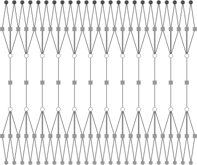
Figure 7: Protograph of spatially-coupled protograph-based (4,2,2,12)-MN codes. The lower protograph with gray circle nodes corresponds to the code used at $\mathsf{S}$, and the upper protograph with dark circle nodes corresponds to the code used at $\mathsf{R}$. The lower and upper protographs will be connected at $\mathsf{D}$ for jointly BP decoding. The channel parameters of the gray circle nodes are $\epsilon_{\mbox{\tiny\sf SD}}$ and those of the dark circle nodes are $\epsilon_{\mbox{\tiny\sf RD}}$.

Figure 8: Achievable erasure probability region of spatially-coupled protograph-based (4,2,2,128)-MN codes at $\mathsf{S}$ and $\mathsf{R}$. The black dashed line represents the theoretical limit Eq. (1) for design rate 0.49609375 and the gray dotted line represents the theoretical limit Eq. (1) for rate 0.5. The achievable region is very close to the theoretical limit. However there still remains a very small gap less than $10^{-4}$ between the boundary of the region and the theoretical limit. This gap is due to wiggles [2].

VI Conclusion

We have designed spatially-coupled protograph-based LDPC and MN codes for erasure relay channels. It is observed that spatially-coupled protograph-based MN codes approach the theoretical limit. We expect that spatially-coupled protograph-based MN codes approach the capacity over the relay channels also with other channel impairments, such that the binary symmetric relay channels and the Gaussian relay channels.

In the future work, we propose spatially-coupled protograph-based MN codes for Gaussian relay channels and prove the rate achievability of the spatially-coupled protographs-based MN codes to the theoretical limit.

References

- [1] A. J. Felström and K. S. Zigangirov, “Time-varying periodic convolutional codes with low-density parity-check matrix,” IEEE Trans. on Inform. Theory, vol. 45, no. 6, pp. 2181–2191, 1999.
- [2] S. Kudekar, T. Richardson, and R. Urbanke, “Threshold saturation via spatial coupling: Why convolutional LDPC ensembles perform so well over the BEC,” IEEE Transactions on Information Theory, vol. 57, no. 2, pp. 803–834, February 2011.
- [3] S. Kudekar, C. Méasson, T. J. Richardson, and R. Urbanke, “Threshold saturation on BMS channels via spatial coupling,” in The 6th International Symposium on Turbo Codes and Related Topics, September 2010, pp. 319–323, brest France.
- [4] E. Arıkan, “Channel polarization: A method for constructing capacity-achieving codes for symmetric binary-input memoryless channels,” IEEE Transactions on Information Theory, vol. 55, no. 7, pp. 3051–3073, 2009.
- [5] T. J. Richardson, M. Shokrollahi, and R. Urbanke, “Design of capacity-approaching irregular low-density parity-check codes,” IEEE Trans. on Inform. Theory, vol. 47, pp. 619–637, 2001.
- [6] S. Kudekar and K. Kasai, “Threshold saturation on channels with memory via spatial coupling,” in IEEE International Symposium on Information Theory (ISIT), August 2011, saint-Petersburg, Russia.
- [7] ——, “Spatially coupled codes over the multiple access channel,” in IEEE International Symposium on Information Theory (ISIT), August 2011, saint-Petersburg, Russia.
- [8] D. MacKay, “Good error-correcting codes based on very sparse matrices,” vol. 45, no. 2, pp. 399 –431, Mar. 1999.
- [9] T. J. Richardson and R. Urbanke, “Multi-edge type LDPC codes,” 2004, http://citeseerx.ist.psu.edu/viewdoc/summary?doi=10.1.1.106.7310.
- [10] T. Murayama, Y. Kabashima, D. Saad, and R. Vicente, “Statistical physics of regular low-density parity-check error-correcting codes,” Phys. Rev. E, vol. 62, no. 2, pp. 1577–1591, 2000.
- [11] T. Tanaka and D. Saad, “Typical performance of regular low-density parity-check codes over general symmetric channels,” J. Phys. A: Math. Gen. , vol. 36, no. 43, pp. 11 143–11 157, 2003.
- [12] K. Kasai and K. Sakaniwa, “Spatial coupling of capacity-achieving codes with bounded density,” in Information Theory and Applications, February 2011, san Diego, USA.
- [13] R. Khalili and K. Salamatian, “On the achievability of cut-set bound for a class of erasure relay channels the non degraded case,” in International Symposium on Information Theory and its Applications (ISITA), October 2004, pp. 269–274, parma, Italy.
- [14] D. Sridhara and C. A. Kelley, “LDPC coding for the three-terminal erasure relay channel,” in IEEE International Symposium on Information Theory (ISIT), 2006, pp. 1229–1233, seattle USA.
- [15] P. Razaghi and W. Yu, “Bilayer low-density parity-check codes for decode-and-forward in relay channels,” IEEE Transactions on Information Theory, vol. 53, no. 10, pp. 3723–3739, 2007.
- [16] T. V. Nguyen, A. Nosratinia, and D. Divsalar, “Bilayer protograph codes for half-duplex relay channels,” in IEEE International Symposium on Information Theory (ISIT), 2010, pp. 948–952.
- [17] V. Savin, “Split-extended LDPC codes for coded cooperation,” in International Symposium on Information Theory and its Applications (ISITA), 2010, pp. 151–156.
- [18] J. Thorpe, “Low Density Parity Check (LDPC) Codes Constructed from Protographs,” JPL IPN Progress Report 42-154, August 2003.
- [19] D. Divsalar, S. Dolinar, C. R. Jones, and K. Andrews, “Capacity-approaching protograph codes.” IEEE Journal on Selected Areas in Communications, vol. 27, no. 6, pp. 876–888, 2009.
- [20] M. Lentmaier, G. Fettweis, K. S. Zigangirov, and D. Costello, “Approaching capacity with asymptotically regular LDPC codes,” in Information Theory and Applications, February 2009, pp. 173–177, san Diego, USA.
- [21] T. J. Richardson and R. Urbanke, Modern Coding Theory. Cambridge University Press, 2008.
- [22] D. Divsalar, C. Jones, S. Dolinar, and J. Thorpe, “Protograph Based LDPC Codes with Minimum Distance Linearly Growing with Block Size,” in IEEE Global Telecommunications Conference (GLOBECOM), November 2005, pp. 1152–1156, st. Louis USA.