Two state scattering problem to Multi-channel scattering problem: Analytically solvable model

Abstract

Starting from few simple examples we have proposed a general method for finding an exact analytical solution for the two state scattering problem in presence of a delta function coupling. We have also extended our model to deal with general one dimensional multi-channel scattering problems.

I Introduction:

Nonadiabatic transition due to potential curve crossing is one of the most important mechanisms to effectively induce electronic transitions in collisions Naka1 . This is a very interdisciplinary concept and appears in various fields of physics and chemistry and even in biology Naka2 ; Naka3 ; Nikitin ; Niki ; Child ; Book . The theory of non-adiabatic transitions dates back to $1932$, when the pioneering works for curve-crossing and non-crossing were published by Landau Landau , Zener Zener and Stueckelberg Stueckelberg and by Rosen and Zener Rosen respectively. Osherov and Voronin solved the case where two diabatic potentials are constant with exponential coupling Voronin . C. Zhu solved the case where two diabatic potentials are exponential with exponential coupling Nikitinmodel . In this paper we consider the case of two or more diabatic potentials with Dirac Delta couplings. The Dirac Delta coupling model has the advantage that it can be exactly solved AniThesis ; AniBook ; Ani1 ; Ani2 ; Ani3 ; Ani4 if the uncoupled diabatic potential has an exact solution.

II Our model:

We consider two diabatic curves, crossing each other. There is a coupling between the two curves, which cause transitions from one curve to another. This transition would occur in the vicinity of the crossing point. In particular, it will occur in a narrow range of x, given by

$$V_{1}(x)-V_{2}(x)\simeq V_{12}(x_{c}),$$ (1)

where $x$ denotes the nuclear coordinate and $x_{c}$ is the crossing point. $V_{1}$ and $V_{2}$ are determined by the shape of the diabatic curves and $V_{12}$ represents the coupling between them. Therefore it is interesting to analyse a model where coupling is localized in space near $x_{c}$. Thus we put

$$V_{12}(x)=K_{0}\delta(x-x_{c}),$$ (2)

where $K_{0}$ is a constant.

Three simple examples

We start with a particle moving on any of the two diabatic curves and the problem is to calculate the probability that the particle will still be on that diabatic curve after a time $t$. We write the probability amplitude for the particle as

$$\Psi(x)=\left(\begin{array}[]{c}\psi_{1}(x)\\ \psi_{2}(x)\end{array}\right),$$ (3)

where $\psi_{1}(x,t)$ and $\psi_{2}(x,t)$ are the probability amplitude for the two states. The Hamiltonian is given by

$$H=\left(\begin{array}[]{cc}H_{11}(x)&V_{12}(x)\\ V_{21}(x)&H_{22}(x)\end{array}\right),$$ (4)

where $H_{1}(x)$, $H_{2}(x)$ and $V_{12}(x)$ are defined by

$$H_{11}(x)=-\frac{1}{2m}\frac{\partial^{2}}{\partial x^{2}}+V_{1}(x),$$ (5)

$$H_{22}(x)=-\frac{1}{2m}\frac{\partial^{2}}{\partial x^{2}}+V_{2}(x)\;\;\text{and}$$

$$V_{12}(x)=V_{21}(x)=K_{0}\delta(x-x_{c}).$$

The above $V_{1}(x)$ and $V_{2}(x)$ are determined by the shape of that diabatic curve. $V(x)$ is a coupling function which we assume to be a Dirac delta function. The time-independent Schr$\stackrel{{\scriptstyle..}}{{o}}$dinger equation is writen in the matrix form

$$\left(\begin{array}[]{cc}H_{11}(x)&V_{12}(x)\\ V_{21}(x)&H_{22}(x)\end{array}\right)\left(\begin{array}[]{c}\psi_{1}(x)\\ \psi_{2}(x)\end{array}\right)=E\left(\begin{array}[]{c}\psi_{1}(x)\\ \psi_{2}(x)\end{array}\right).$$ (6)

This is equivalent to

$$H_{11}(x)\psi_{1}(x)+K_{0}\delta(x-x_{c})\psi_{2}(x)=E\psi_{1}(x)\;\;\;\text{and}$$ (7)

$$K_{0}\delta(x-x_{c})\psi_{1}(x)+H_{22}(x)\psi_{2}(x)=E\psi_{2}(x).$$

Integrating the above two equations from $x_{c}-\eta$ to $x_{c}+\eta$ (where $\eta\rightarrow 0$) we get we get the following two boundary conditions

$$-\frac{\hbar^{2}}{2m}\left[\frac{d\psi_{1}(x)}{dx}\right]_{x_{c}-\eta}^{x_{c}+\eta}+K_{0}\psi_{2}(x_{c})=0\;\;\;\text{and}$$ (8)

$$-\frac{\hbar^{2}}{2m}\left[\frac{d\psi_{2}(x)}{dx}\right]_{x_{c}-\eta}^{x_{c}+\eta}+K_{0}\psi_{1}(x_{c})=0.$$

Also we have two more boundary condition

$$\psi_{1}(x_{c}-\eta)=\psi_{1}(x_{c}+\eta)\;\;\;\;\text{and}$$ (9)

$$\psi_{2}(x_{c}-\eta)=\psi_{2}(x_{c}+\eta).$$

Using the above four boundary conditions we derive the transition probability from one diabatic potential to the other, in the case of coupling between (a) two constant potentials, (b) two linear potentials and (c) two exponential potential.

Exact analytical solution for constant potential case:

In region 1 $(x<x_{c})$, the time-independent Schr$\stackrel{{\scriptstyle..}}{{o}}$dinger equation for the first potential is given by

$$-\frac{1}{2m}\frac{\partial^{2}\psi_{1}(x)}{\partial x^{2}}=E\psi_{1}(x).$$ (10)

The above equation has the following solution

$$\psi_{1}(x)=Ae^{ik_{1}x}+Be^{-ik_{1}x},$$ (11)

where $k_{1}=\sqrt{\frac{2m}{\hbar^{2}}E}$. In region 2 $(x>x_{c})$, the time-independent Schr$\stackrel{{\scriptstyle..}}{{o}}$dinger equation for the first potential is given by

$$-\frac{1}{2m}\frac{\partial^{2}\psi_{1}(x)}{\partial x^{2}}=E\psi_{1}(x)_{1}(x)$$ (12)

Physically acceptable solution of the above equation is given by

$$\psi_{1}(x)=Ce^{ik_{1}x}.$$ (13)

In region 1 $(x<x_{c})$, the time independent Schr$\stackrel{{\scriptstyle..}}{{o}}$dinger equation for the second potential is given by

$$-\frac{1}{2m}\frac{\partial^{2}\psi_{2}(x)}{\partial x^{2}}+V_{2}\psi_{2}(x)=E\psi_{2}(x).$$ (14)

Physically acceptable solution is given by

$$\psi_{2}(x)=De^{-ik_{2}x},$$ (15)

where $k_{2}=\sqrt{\frac{2m}{\hbar^{2}}(E-V_{2})}$. In region 2 $(x>x_{c})$, the time-independent Schr$\stackrel{{\scriptstyle..}}{{o}}$dinger equation for the second potential is given by

$$-\frac{1}{2m}\frac{\partial^{2}\psi_{2}(x)}{\partial x^{2}}+V_{2}\psi_{2}(x)=E\psi_{2}(x).$$ (16)

Physically acceptable solution is given by

$$\psi_{2}(x)=Fe^{ik_{2}x}.$$ (17)

Here we put $x_{c}=0$. Now using four boundary conditions we calculate

$$\left|\frac{F}{A}\right|^{2}=\left|\frac{imK_{0}k_{1}\hbar^{2}}{(k_{1}k_{2}\hbar^{4}+m^{2}K_{0}^{2})}\right|^{2}.$$ (18)

and

$$\left|\frac{D}{A}\right|^{2}=\left|\frac{imK_{0}k_{1}\hbar^{2}}{(k_{1}k_{2}\hbar^{4}+m^{2}K_{0}^{2})}\right|^{2}.$$ (19)

So, the transition probability is given by

$$T=2\frac{k_{2}}{k_{1}}\left|\frac{imK_{0}k_{1}\hbar^{2}}{(k_{1}k_{2}\hbar^{4}+m^{2}K_{0}^{2})}\right|^{2}.$$ (20)

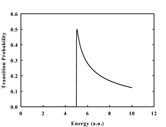
Figure 1: The plot of transition probability from one constant potential to another constant potential as a function of energy of incident particle ($K_{0}$=1.0).

In our numerical calculation we use atomic units so that $\hbar=1$. In the atomic units, we set $V_{1}(x)=0$, $V_{2}(x)=5$, $K_{0}=1.0$ and $m=1.0$. The result of our calculation is shown in Fig. 1.

Exact analytical solution for Linear potential case:

The time-independent Schr$\stackrel{{\scriptstyle..}}{{o}}$dinger equation for the case where a linear potential coupled to another linear potential through a Dirac delta interaction is given below (see Fig. 2).

$$\left(\begin{array}[]{cc}-\frac{1}{2m}\frac{\partial^{2}}{\partial x^{2}}+p_{1}x&K_{0}\delta(x-x_{c})\\ K_{0}\delta(x-x_{c})&-\frac{1}{2m}\frac{\partial^{2}}{\partial x^{2}}-p_{2}x\end{array}\right)\left(\begin{array}[]{c}\psi_{1}(x)\\ \psi_{2}(x)\end{array}\right)=E\left(\begin{array}[]{c}\psi_{1}(x)\\ \psi_{2}(x)\end{array}\right).$$ (21)

The Eq. (21) can be split into two equations

Figure 2: Schematic diagram of the two state problem, where one linear potential is coupled to another linear potential in the diabatic representation.

$$\left(-\frac{1}{2m}\frac{\partial^{2}}{\partial x^{2}}+p_{1}x\right)\psi_{1}(x)+K_{0}\delta(x)\psi_{2}(x)=E\psi_{1}(x)\;\;\;\text{and}$$ (22)

$$\left(-\frac{1}{2m}\frac{\partial^{2}}{\partial x^{2}}-p_{2}x\right)\psi_{2}(x)+K_{0}\delta(x)\psi_{1}(x)=E\psi_{2}(x).$$

In our calculation, we use $p_{1}=p_{2}=1$. The Time-independent Schr$\stackrel{{\scriptstyle..}}{{o}}$dinger equation for the first diabatic potential is given below,

$$\left(-\frac{1}{2m}\frac{\partial^{2}}{\partial x^{2}}+x\right)\psi_{1}(x)=E\psi_{1}(x).$$ (23)

In region 1 ( $x<x_{c}$) the physically acceptable solution is given below

$$\psi_{1}(x)=(A+B)A_{i}\left[2^{\frac{1}{3}}(-E+x)\right]+i(A-B)A_{i}\left[2^{\frac{1}{3}}(-E+x)\right].$$ (24)

Here $A_{i}[z]$ and $B_{i}[z]$ represent the Airy functions. In the above expression $A$ denotes the probability amplitude for motion along the positive direction and $B$ denotes the probability amplitude for motion along the negative direction Ani5 . The physically acceptable solution in region 2 ( $x>x_{c}$), is given by

$$\psi_{1}(x)=CA_{i}\left[2^{\frac{1}{3}}(-E+x)\right].$$ (25)

In this region the net flux is zero Ani5 .

The time-independent Schr$\stackrel{{\scriptstyle..}}{{o}}$ dinger equation for the second diabatic potential is given below

$$\left(-\frac{1}{2m}\frac{\partial^{2}}{\partial x^{2}}-x\right)\psi_{2}(x)=E\psi_{2}(x).$$ (26)

In region1 ( $x<x_{c}$) the physically acceptable solution is

$$\psi_{2}(x)=DA_{i}\left[2^{\frac{1}{3}}(-E-x)\right].$$ (27)

In this region the net flux is zero Ani5 . In region 2 ( $x>x_{c}$) the physically acceptable solution is

$$\psi_{2}(x)=F\left(A_{i}\left[2^{\frac{1}{3}}(-E-x)\right]-iB_{i}\left[2^{\frac{1}{3}}(-E-x)\right]\right).$$ (28)

Using the four boundary conditions mentioned above (here we put $x_{c}=0$), we have derived an analytical expression for the transition probability from one diabatic potential to the other diabatic potential and the final expression is given below

$$T=16\times 2^{2/3}\left|\frac{N}{D}\right|^{2},$$ (29)

where

$$N=Ai\left[-2^{1/3}E\right]^{2}\left(-Ai^{\prime}\left[-2^{1/3}E\right]Bi\left[-2^{1/3}E\right]+Ai\left[-2^{1/3}E\right]Bi^{\prime}\left[-2^{1/3}E\right]\right)$$ (30)

and

$$D=-8iAi\left[-2^{1/3}E\right]^{3}Bi\left[-2^{1/3}E\right]+2^{2/3}Ai^{\prime}\left[-2^{1/3}E\right]^{2}Bi\left[-2^{1/3}E\right]^{2}$$ (31)

$$+4Ai\left[-2^{1/3}E\right]^{4}-22^{2/3}Ai\left[-2^{1/3}E\right]Ai^{\prime}\left[-2^{1/3}E\right]Bi\left[-2^{1/3}E\right]Bi^{\prime}\left[-2^{1/3}E\right]$$

$$+Ai\left[-2^{1/3}E\right]^{2}\left(-4Bi\left[-2^{1/3}E\right]^{2}+2^{2/3}Bi^{\prime}\left[-2^{1/3}E\right]^{2}\right).$$

In our numerical calculation we set $p_{1}=1$, $p_{2}=1$, $K_{0}=1$ and $m=1$ in atomic units. The result of our calculation is shown in Fig. 3.

Figure 3: The plot of transition probability from one linear potential to another linear potential, as a function of energy of incident particle ($K_{0}$=1.0).

Exact analytical solution for exponential potential case:

We start with the time-independent Schr$\stackrel{{\scriptstyle..}}{{o}}$dinger equation for a two state system

$$\left(\begin{array}[]{cc}-\frac{1}{2m}\frac{\partial^{2}}{\partial x^{2}}+V_{0}e^{ax}&K_{0}\delta(x-x_{c})\\ K_{0}\delta(x-x_{c})&-\frac{1}{2m}\frac{\partial^{2}}{\partial x^{2}}+V_{0}e^{-ax}\end{array}\right)\left(\begin{array}[]{c}\psi_{1}(x)\\ \psi_{2}(x)\end{array}\right)=E\left(\begin{array}[]{c}\psi_{1}(x)\\ \psi_{2}(x)\end{array}\right).$$ (32)

Eq. (32) can be split into the following two equations

$$\left(-\frac{1}{2m}\frac{\partial^{2}}{\partial x^{2}}+V_{0}e^{ax}\right)\psi_{1}(x)+K_{0}\delta(x-x_{c})\psi_{2}(x)=E\psi_{1}(x)\;\;\;\text{and}$$ (33)

$$\left(-\frac{1}{2m}\frac{\partial^{2}}{\partial x^{2}}+V_{0}e^{-ax}\right)\psi_{2}(x)+K_{0}\delta(x-x_{c})\psi_{1}(x)=E\psi_{2}(x).$$

In our calculation we took $V_{0}=1.0$ and $a=1$. Using the time-independent Schr$\stackrel{{\scriptstyle..}}{{o}}$dinger equation the first diabatic potential is given below

Figure 4: Schematic diagram of the two state problem, where one exponential potential is coupled to another exponential potential in the diabatic representation.

$$\left(-\frac{1}{2m}\frac{\partial^{2}}{\partial x^{2}}+V_{0}e^{ax}\right)\psi_{1}(x)=E\psi_{1}(x).$$ (34)

In the region $x<x_{c}$, the solution of the above equation is given below

$$\psi_{1}(x)=A\,I_{(2\,i\,\sqrt{2E}\,)}(2\,\sqrt{2e^{x}})\,+B\,I_{(-2\,i\,\sqrt{2E}\,)}(2\,\sqrt{2e^{x}})\,.$$ (35)

Here $I_{n}(z)$ represent the modified Bessel function of the first kind. In the above expression $A$ denotes the probability amplitude for motion along the positive direction and $B$ denotes the probability amplitude for motion along the negative direction Ani5 . In the region, where $x>x_{c}$, the physically acceptable solution is

$$\psi_{1}(x)=CK_{(-2\,i\,\sqrt{2E}\,)}(2\,\sqrt{2e^{x}}).$$ (36)

Here $K_{n}(z)$ represent the modified Bessel function of the second kind. In this region the net flux is zero Ani3 .

For the second diabatic potential, the time-independent Schr$\stackrel{{\scriptstyle..}}{{o}}$dinger equation is given below

$$\left(-\frac{1}{2m}\frac{\partial^{2}}{\partial x^{2}}+V_{0}e^{-ax}\right)\psi_{2}(x)=E\psi_{2}(x).$$ (37)

In the region, where $x>x_{c}$, the physically acceptable solution is

$$\psi_{2}(x)=F\,I_{(-2\,i\,\sqrt{2E}\,)}(2\,\sqrt{2e^{-x}}).$$ (38)

In the region, where $x<x_{c}$, the physically acceptable solution is

$$\psi_{2}(x)=DK_{(-2\,i\,\sqrt{2E}\,)}(2\,\sqrt{2e^{x}}).$$ (39)

In this region the net flux is zero Ani3 . Using four boundary conditions and putting $x_{c}=0$, as mentioned before, we derive an expression for transition probability from one exponential potential to the other exponential potential. In our numerical calculation we use atomic unit. The value of $K_{0}=0.1$ and $m=1$. The result of our calculation is shown in Fig. 5.

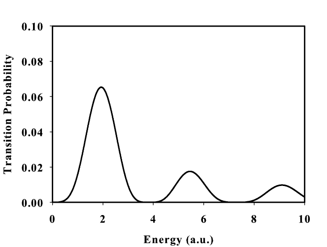
Figure 5: The plot of transition probability from one exponential potential to the other as a function of energy of incident particle ($K_{0}$=0.1).

III Formulation of general solution for two state scattering problem using our model

We start with the time-independent Schr$\stackrel{{\scriptstyle..}}{{o}}$dinger equation for a two state system

$$\left(\begin{array}[]{cc}H_{11}(x)&V_{12}(x)\\ V_{21}(x)&H_{22}(x)\end{array}\right)\left(\begin{array}[]{c}\psi_{1}(x)\\ \psi_{2}(x)\end{array}\right)=E\left(\begin{array}[]{c}\psi_{1}(x)\\ \psi_{2}(x)\end{array}\right).$$ (40)

This equation can be written in the following form

$$\psi_{2}(x)=V_{12}(x)^{-1}\left[E-H_{11}(x)\right]\psi_{1}(x)\;\;\;\text{and}$$ (41)

$$\psi_{2}(x)=\left[E-H_{22}(x)\right]^{-1}V_{21}(x)\psi_{1}(x).$$

Eliminating $\psi_{2}(x)$ from the above two equations we get

$$\left[E-H_{11}(x)\right]\psi_{1}(x)-V_{12}(x)\left[E-H_{22}(x)\right]^{-1}V_{21}(x)\psi_{1}(x)=0.$$ (42)

The above equations simplify considerably if $V_{12}(x)$ and $V_{21}(x)$ are Dirac Delta function at $x_{c}$, which in operator notation may be written as $V=$ $K_{0}S=K_{0}$ $|x_{c}\rangle$ $\langle x_{c}|$. The above equation now become

$$\left(\left[E-H_{11}(x)\right]-K_{0}^{2}|x_{c}\rangle\langle x_{c}|\left[E-H_{22}(x)\right]^{-1}|x_{c}\rangle\langle x_{c}|\right)\psi_{1}(x)=0.$$ (43)

This may be written as

$$\left[H_{11}(x)+K_{0}^{2}\delta(x-x_{c})G_{2}^{0}(x_{c},x_{c};E)\right]\psi_{1}(x)=E\psi_{1}(x).$$ (44)

The above equation can be written in the following form

$$\left[E-H_{11}\right]\psi_{1}(x)=K_{0}^{2}\delta(x-x_{c})G_{2}^{0}(x_{c},x_{c};E)\psi_{1}(x),$$ (45)

where the right hand side is considered as an inhomogeneous term. The general solution of this equation can be written as

$$\psi_{1}(x)=\psi_{0}(x)+K_{0}^{2}G_{1}^{0}(x,x_{c};E)G_{2}^{0}(x_{c},x_{c};E)\psi_{1}(x_{c}),$$ (46)

where $\psi_{0}(x)$ is a solution of the homogeneous equation

$$\left[E-H_{11}\right]\psi_{0}(x)=0\;\;\;\text{and}$$ (47)

$$\left[E-H_{11}\right]G_{1}^{0}(x,x^{\prime};E)=\delta(x-x^{\prime}).$$

In the above equation

$$\psi_{1}(x)=\int\limits_{-\infty}^{\infty}dx^{\prime}G(x,x^{\prime};E)\psi_{0}(x^{\prime})\;\;\;\text{and}$$ (48)

$$\psi_{0}(x)=\int\limits_{-\infty}^{\infty}dx^{\prime}G_{1}^{0}(x,x^{\prime};E)\psi_{0}(x^{\prime}).$$

So Eq. (46) can be written as

$$\begin{array}[]{c}\int\limits_{-\infty}^{\infty}dx^{\prime}G(x,x^{\prime};E)\psi_{0}(x^{\prime})=\int\limits_{-\infty}^{\infty}dx^{\prime}G_{1}^{0}(x,x^{\prime};E)\psi_{0}(x^{\prime})\\ +K_{0}^{2}G_{1}^{0}(x,x_{c};E)G_{2}^{0}(x_{c},x_{c};E)\int\limits_{-\infty}^{\infty}dx^{\prime}G(x_{c},x^{\prime};E)\psi_{0}(x^{\prime}).\end{array}$$ (49)

The solution in terms of Green’s function is as follows

$$G(x,x^{\prime};E)=G_{1}^{0}(x,x^{\prime};E)+K_{0}^{2}G_{1}^{0}(x,x_{c};E)G_{2}^{0}(x_{c},x_{c};E)G(x_{c},x^{\prime};E).$$ (50)

In the above equation we put $x=x_{c}$

$$G(x_{c},x^{\prime};E)=G_{1}^{0}(x_{c},x^{\prime};E)+K_{0}^{2}G_{1}^{0}(x_{c},x_{c};E)G_{2}^{0}(x_{c},x_{c};E)G(x_{c},x^{\prime};E).$$ (51)

After simplification, we get

$$G(x_{c},x^{\prime};E)=\frac{G_{1}^{0}(x_{c},x^{\prime};E)}{1-K_{0}^{2}G_{1}^{0}(x_{c},x_{c};E)G_{2}^{0}(x_{c},x_{c};E)},$$ (52)

so that

$$G(x,x^{\prime};E)=G_{1}^{0}(x,x^{\prime};E)+\frac{K_{0}^{2}G_{1}^{0}(x,x_{c};E)G_{2}^{0}(x_{c},x_{c};E)G_{1}^{0}(x_{c},x^{\prime};E)}{1-K_{0}^{2}G_{1}^{0}(x_{c},x_{c};E)G_{2}^{0}(x_{c},x_{c};E)}.$$ (53)

In the above expression, we have the Green’s function for two state scattering problem using delta function coupling model. Using the expression of $G(x,x^{\prime};E)$ one can calculate wave function and from the wave function one can easily calculate the transition probability from one diabatic potential to the other.

Three channel scattering problem using our model

We start with a particle moving on any of the three diabatic curves and the problem is to calculate the probability that the particle will still be in that diabatic curve after a time $t$. We write the probability amplitude for the particle as

$$\Psi(x)=\left(\begin{array}[]{c}\psi_{1}(x)\\ \psi_{2}(x)\\ \psi_{3}(x)\end{array}\right).$$ (54)

Where $\psi_{1}(x,t)$, $\psi_{2}(x,t)$ and $\psi_{3}(x)$ are the probability amplitude for the three states. The Hamiltonian matrix of this system is given by

$$H=\left(\begin{array}[]{ccc}H_{11}(x)&V_{12}(x)&V_{13}(x)\\ V_{21}(x)&H_{22}(x)&0\\ V_{31}(x)&0&H_{33}(x)\end{array}\right),$$ (55)

where $H_{1}(x)$, $H_{2}(x)$, $H_{3}(x)$, $V_{12}(x)$, $V_{21}(x)$, $V_{31}(x)$ and $V_{13}(x)$ are defined by

$$H_{11}(x)=-\frac{1}{2m}\frac{\partial^{2}}{\partial x^{2}}+V_{1}(x),$$ (56)

$$H_{22}(x)=-\frac{1}{2m}\frac{\partial^{2}}{\partial x^{2}}+V_{2}(x),$$

$$H_{33}(x)=-\frac{1}{2m}\frac{\partial^{2}}{\partial x^{2}}+V_{3}(x),$$

$$V_{12}(x)=V_{21}(x)=K_{0}\delta(x-x_{c})\;\;\;\text{and}$$

$$V_{13}(x)=V_{31}(x)=K_{0}\delta(x-x_{c}).$$

In the above equation $V_{1}(x)$, $V_{2}(x)$ and $V_{3}(x)$ are determined by the shape of that diabatic curve. The time-independent Schr$\stackrel{{\scriptstyle..}}{{o}}$dinger equation for this problem is given by

$$\left(\begin{array}[]{ccc}H_{11}(x)&K_{0}\delta(x-x_{c})&K_{0}\delta(x-x_{c})\\ K_{0}\delta(x-x_{c})&H_{22}(x)&0\\ K_{0}\delta(x-x_{c})&0&H_{33}(x)\end{array}\right)\left(\begin{array}[]{c}\psi_{1}(x)\\ \psi_{2}(x)\\ \psi_{3}(x)\end{array}\right)=E\left(\begin{array}[]{c}\psi_{1}(x)\\ \psi_{2}(x)\\ \psi_{3}(x)\end{array}\right).$$ (57)

This matrix representation is equivalent to the following three equations

$$H_{11}(x)\psi_{1}(x)+K_{0}\delta(x-x_{c})\psi_{2}(x)+K_{0}\delta(x-x_{c})\psi_{3}(x)=E\psi_{1}(x),$$ (58)

$$K_{0}\delta(x-x_{c})\psi_{1}(x)+H_{22}(x)\psi_{2}(x)=E\psi_{2}(x)\;\;\text{and}$$

$$K_{0}\delta(x-x_{c})\psi_{1}(x)+H_{33}(x)\psi_{3}(x)=E\psi_{3}(x).$$

Integrating the above three equations from $x_{c}-\eta$ to $x_{c}+\eta$ (where $\eta\rightarrow 0$) we get the following three boundary conditions

$$-\frac{\hbar^{2}}{2m}\left[\frac{d\psi_{1}(x)}{dx}\right]_{x_{c}-\eta}^{x_{c}+\eta}+K_{0}\psi_{2}(x_{c})+K_{0}\psi_{3}(x_{c})=0,$$ (59)

$$-\frac{\hbar^{2}}{2m}\left[\frac{d\psi_{2}(x)}{dx}\right]_{x_{c}-\eta}^{x_{c}+\eta}+K_{0}\psi_{1}(x_{c})=0\;\;\text{and}$$

$$-\frac{\hbar^{2}}{2m}\left[\frac{d\psi_{3}(x)}{dx}\right]_{x_{c}-\eta}^{x_{c}+\eta}+K_{0}\psi_{1}(x_{c})=0.$$

Also we have three more boundary conditions

$$\psi_{1}(x_{c}-\eta)=\psi_{1}(x_{c}+\eta)$$ (60)

$$\psi_{2}(x_{c}-\eta)=\psi_{2}(x_{c}+\eta)\;\;\text{and}$$

$$\psi_{3}(x_{c}-\eta)=\psi_{3}(x_{c}+\eta).$$

Using the above six boundary conditions we derive analytical expressions for transition probability from one diabatic potential to the other in the case of coupling between (a) three constant potentials, (b) three linear potentials and (c) three exponential potentials.

IV Formulation of general solution for multi-channel scattering problem using our model

We start with the time-independent Schr$\stackrel{{\scriptstyle..}}{{o}}$dinger equation for a three state system, given by

$$\left(\begin{array}[]{ccc}H_{11}(x)&V_{12}(x)&V_{13}(x)\\ V_{21}(x)&H_{22}(x)&0\\ V_{31}(x)&0&H_{33}(x)\end{array}\right)\left(\begin{array}[]{c}\psi_{1}(x)\\ \psi_{2}(x)\\ \psi_{3}(x)\end{array}\right)=E\left(\begin{array}[]{c}\psi_{1}(x)\\ \psi_{2}(x)\\ \psi_{3}(x)\end{array}\right),$$ (61)

where

$$H_{11}(x)=-\frac{1}{2m}\frac{\partial^{2}}{\partial x^{2}}+V_{1}(x),$$ (62)

$$H_{22}(x)=-\frac{1}{2m}\frac{\partial^{2}}{\partial x^{2}}+V_{2}(x)\;\;\text{and}$$

$$H_{33}(x)=-\frac{1}{2m}\frac{\partial^{2}}{\partial x^{2}}+V_{3}(x).$$

This above matrix equation can be written in the following form

$$\left[H_{11}(x)-E\right]\psi_{1}(x)+V_{12}(x)\psi_{2}(x)+V_{13}(x)\psi_{3}(x)=0,$$ (63)

$$\left[H_{22}(x)-E\right]\psi_{2}(x)+V_{21}(x)\psi_{1}(x)=0\;\;\text{and}$$

$$\left[H_{33}(x)-E\right]\psi_{3}(x)+V_{31}(x)\psi_{1}(x)=0.$$

The above equation after rearranging is given below

$$\left[E-H_{11}(x)\right]\psi_{1}(x)-V_{12}(x)\psi_{2}(x)-V_{13}(x)\psi_{3}(x)=0,$$ (64)

$$\psi_{2}(x)=\left[E-H_{22}(x)\right]^{-1}V_{21}(x)\psi_{1}(x)\;\;\text{and}$$ (65)

$$\psi_{3}(x)=\left[E-H_{33}(x)\right]^{-1}V_{31}(x)\psi_{1}(x).$$ (66)

After eliminating both $\psi_{2}(x)$ and $\psi_{3}(x)$ from Eq. (97) we get

$$\left(\left[E-H_{11}(x)\right]-V_{12}(x)\left[E-H_{22}(x)\right]^{-1}V_{21}(x)-V_{13}(x)\left[E-H_{33}(x)\right]^{-1}V_{31}(x)\right)\psi_{1}(x)=0.$$ (67)

The above equations are true for any general $V_{12}$, $V_{21}$, $V_{13}$ and $V_{31}$. The above equation simplify considerably if $V_{12}$, $V_{13}$, $V_{31}$ and $V_{21}$ are Dirac Delta functions, which we write in operator notation as $V_{12}=V_{21}=K_{2}S=K_{2}|x_{2}\rangle\langle x_{2}|$ and $V_{13}=V_{31}=K_{3}S=K_{3}|x_{3}\rangle\langle x_{3}|$. The above equation now becomes

$$\left(\left[E-H_{11}(x)\right]-K_{2}^{2}\delta(x-x_{2})G_{2}^{0}(x_{2},x_{2};E)-K_{3}^{2}\delta(x-x_{3})G_{2}^{0}(x_{3},x_{3};E)\right)\psi_{1}(x)=0.$$ (68)

This may be written as

$$\left(\left[E-H_{12}(x)\right]-K_{3}^{2}\delta(x-x_{3})G_{3}^{0}(x_{3},x_{3};E)\right)\psi_{1}(x)=0,$$ (69)

where

$$H_{12}(x)=H_{11}(x)+K_{2}^{2}\delta(x-x_{2})G_{2}^{0}(x_{2},x_{2};E).$$ (70)

For $H_{12}(x)$, one can find the corresponding Green’s function $G_{12}(x,x^{\prime};E)$ using the method as we have used in two state case.

$$\left[E-H_{11}\right]\psi_{1}(x)=K_{2}^{2}\delta(x-x_{2})G_{2}^{0}(x_{2},x_{2};E)\psi_{1}(x),$$ (71)

where the right hand side is considered as an inhomogeneous term. The general solution of this equation can be written as

$$\psi_{1}(x)=\psi_{0}(x)+\int\limits_{-\infty}^{\infty}dxG_{1}^{0}(x,x^{\prime};E)K_{2}^{2}\delta(x^{\prime}-x_{2})G_{2}^{0}(x_{2},x_{2};E)\psi_{1}(x^{\prime}),$$ (72)

where $\psi_{0}(x)$ is a solution of the homogeneous equation

$$(E-H_{11})\psi_{0}(x)=0,$$ (73)

where

$$(E-H_{11})G_{1}^{0}(x,x^{\prime};E)=\delta(x-x^{\prime}).$$ (74)

So

$$\psi_{1}(x)=\psi_{0}(x)+K_{2}^{2}G_{1}^{0}(x,x_{2};E)G_{2}^{0}(x_{2},x_{2};E)\psi_{1}(x_{2}).$$ (75)

In the above expression

$$\psi_{1}(x)=\int\limits_{-\infty}^{\infty}dx^{\prime}G_{12}(x,x^{\prime};E)\psi_{0}(x^{\prime})\;\;\text{and}$$ (76)

$$\psi_{0}(x)=\int\limits_{-\infty}^{\infty}dx^{\prime}G_{1}^{0}(x,x^{\prime};E)\psi_{0}(x^{\prime}).$$

So Eq. (108) can be written as
$\int\limits_{-\infty}^{\infty}dx^{\prime}G_{12}(x,x^{\prime};E)\psi_{0}(x^{\prime})$=

$$\int\limits_{-\infty}^{\infty}dx^{\prime}G_{1}^{0}(x,x^{\prime};E)\psi_{0}(x^{\prime})+K_{2}^{2}G_{1}^{0}(x,x_{2};E)G_{2}^{0}(x_{2},x_{2};E)\int\limits_{-\infty}^{\infty}dx^{\prime}G_{12}(x_{2},x^{\prime};E)\psi_{0}(x^{\prime}).$$ (77)

The solution in terms of Green’s function, extracted from last equation

$$G_{12}(x,x^{\prime};E)=G_{1}^{0}(x,x^{\prime};E)+K_{2}^{2}G_{1}^{0}(x,x_{2};E)G_{2}^{0}(x_{2},x_{2};E)G_{12}(x_{2},x^{\prime};E).$$ (78)

In the above equation we put $x=x_{2}$ to get

$$G_{12}(x_{2},x^{\prime};E)=G_{1}^{0}(x_{2},x^{\prime};E)+K_{2}^{2}G_{2}^{0}(x_{2},x_{2};E)G_{1}^{0}(x_{2},x_{2};E)G_{12}(x_{2},x^{\prime};E).$$ (79)

So after simplification we get

$$G_{12}(x_{2},x^{\prime};E)=\frac{G_{1}^{0}(x_{2},x^{\prime};E)}{1-K_{2}^{2}G_{1}^{0}(x_{2},x_{2};E)G_{2}^{0}(x_{2},x_{2};E)},$$ (80)

so that

$$G_{12}(x,x^{\prime};E)=G_{1}^{0}(x,x^{\prime};E)+\frac{K_{2}^{2}G_{1}^{0}(x,x_{2};E)G_{2}^{0}(x_{2},x_{2};E)G_{1}^{0}(x_{2},x^{\prime};E)}{1-K_{2}^{2}G_{1}^{0}(x_{2},x_{2};E)G_{2}^{0}(x_{2},x_{2};E)}$$ (81)

Now we will incorporate the effect of third state which is coupled to first state only, i.e. we will solve Eq. (102) in terms of Greens function.

$$G_{13}(x,x^{\prime};E)=G_{12}(x,x^{\prime};E)+\frac{K_{2}^{2}G_{12}(x,x_{3};E)G_{2}^{0}(x_{3},x_{3};E)G_{12}(x_{3},x^{\prime};E)}{1-K_{2}^{2}G_{12}(x_{3},x_{3};E)G_{2}^{0}(x_{3},x_{3};E)}$$ (82)

So after incorporating $N$-th state, where all states are coupled to the first one only we will get

$$((E-H_{1[N-1]}(x))-K_{N}^{2}\delta(x-x_{N})G_{N}^{0}(x_{N},x_{N};E))\psi_{1}(x)=0,$$ (83)

where

$$H_{1[N-1]}(x)=H_{11}(x))+\sum\limits_{n=2}^{N-1}K_{n}^{2}\delta(x-x_{n})G_{n}^{0}(x_{n},x_{n};E).$$ (84)

In this case, one can find the Green’s function $G_{1N}(x,x^{\prime};E)$ using the method as we have already used.

$$G_{1N}(x,x^{\prime};E)=G_{1[N-1]}(x,x^{\prime};E)+\frac{K_{2}^{2}G_{1[N-1]}(x,x_{N};E)G_{N}^{0}(x_{N},x_{N};E)G_{1[N-1]}(x_{N},x^{\prime};E)}{1-K_{2}^{2}G_{1[N-1]}(x_{N},x_{N};E)G_{N}^{0}(x_{N},x_{N};E)}.$$ (85)

In this case we can calculate $G_{1N}(x,x_{0};E)$ if we know $G_{1(N-1)}(x,x_{0};E)$. So using $G_{1N}(x,x_{0};E)$, one can calculate wave function explicitely and from the wave function one can easily calculate transition probability from one diabatic potential to all other diabatic potentials.

V Conclusions:

Starting from few simple examples, we have proposed a general method for finding the exact analytical solution for the two state quantum scattering problem in presence of a delta function coupling. Our solution is quite general and is valid for any potential. We have also extended our model to deal with general one dimensional multi-channel scattering problems. The same procedure is also applicable to the case where $S$ is a non-local operator and may be represented by $S\equiv|f\rangle$ $K_{0}$ $\langle g|$, where $f$ and $g$ are arbitrary acceptable functions. Choosing both of them to be Gaussian should be an improvement over the delta function coupling model. $S$ may even be a linear combination of such operators.

VI Acknowledgments:

It is a pleasure to thank Prof. K. L. Sebastian for suggesting this problem. The author would like to thank Prof. M. S. Child for his kind interest, suggestions and encouragement.

References

- (1) H. Nakamura, Int. Rev. Phys. Chem., 10, 123 (1991).
- (2) H. Nakamura, in Theory, Advances in Chemical Physics, edited by M. Bayer and C. Y. Ng (John Wiley and Sons, New York, 1992).
- (3) H. Nakamura, Nonadiabatic Transition, (World Scientific, Singapore, 2002).
- (4) E. E. Nikitin and S. Ia. Umanskii, Theory of Slow Atomic Collisions, (Springer, Berlin, 1984).
- (5) E. E. Nikitin, Ann. Rev. Phys. Chem. 50, 1 (1999).
- (6) M. S. Child, Molecular Collision Theory, (Dover, Mineola, NY, 1996).
- (7) E.S. Medvedev and V.I. Osherov, Radiationless Transitions in Polyatomic Molecules, (Springer, New York, 1994).
- (8) L. D. Landau, Phys. Zts. Sowjet., 2,46 (1932).
- (9) C. Zener, Proc. Roy. Soc. A, 137, (1932) 696.
- (10) E. C. G. Stuckelberg, Helv. Phys. Acta, 5,369 (1932) .
- (11) N. Rosen and C. Zener, Phys. Rev., 40,502 (1932).
- (12) V. I. Osherov and A. I. Veronin, Phys. Rev. A, 49,265 (1994).
- (13) C. Zhu, J. Phys. A, 29,1293(1996).
- (14) A. Chakraborty, Ph.D. Thesis, (Indian Institute of Science, India, 2004).
- (15) A. Chakraborty, Nano Devices, 2D Electron Solvation and Curve Crossing Problems: Theoretical Model Investigations, (LAMBERT Academic Publishing, Germany, 2010).
- (16) A. Chakraborty, Mol. Phys. 107, 165 (2009).
- (17) A. Chakraborty, Mol. Phys. 107, 2459 (2009).
- (18) A. Chakraborty, Mol. Phys. 109, 429 (2011).
- (19) A. Chakraborty, Mol. Phys. (under revision) (2011).
- (20) A. Chakraborty, (unpublished).