On the thermalization of a Luttinger liquid after a sequence of sudden interaction quenches

Abstract

We present a comprehensive analysis of the relaxation dynamics of a Luttinger liquid subject to a sequence of sudden interaction quenches. We express the critical exponent $\beta$ governing the decay of the steady-state propagator as an explicit functional of the switching protocol. At long distances $\beta$ depends only on the initial state while at short distances it is also history dependent. Continuous protocols of arbitrary complexity can be realized with infinitely long sequences. For quenches of finite duration we prove that there exist no protocol to bring the initial non-interacting system in the ground state of the Luttinger liquid. Nevertheless memory effects are washed out at short-distances. The adiabatic theorem is then investigated with ramp-switchings of increasing duration, and several analytic results for both the propagator and the excitation energy are derived.

I Introduction

The on-going experimental activities on ultracold atoms are continuously challenging our understanding of many-body quantum systems.new Laser- or evaporative-cooled below the $\mu$K, atoms crystallize in artificial latticesrev thus providing nearly ideal realizations of bosonicopt1 ; opt11 ; opt1a ; opt1b and fermionicopt22 ; opt2a ; opt2b model Hamiltonians. The possibility of tuning the model parameters in real time brought the attention back to a fundamental issue in quantum statistical physics: does a non-interacting bulk system relax toward the correlated ground-state upon the switch-on of the interaction?

“Sudden quench” is the nomenclature coined for the sudden change of a parameter like, e.g., the convexity of a parabolic trap or the interaction strength, in an equilibrium system.koll ; man During the last five years experimental and theoretical investigations on the relaxation properties of quenched ultracold atoms enlightened the intriguing phenomenon of the thermalization breakdown:thermb either the system does not reach a steady state or, if it does, the steady state is not the ground state of the quenched Hamiltonian. A sufficient criterion for the occurrence of a steady-state has been found, so far, only for integrable modelsbs.2008 ; stef ; s.2007 ; c.2009 and it has been argued that steady-state values are calculable by averaging over a generalized, initial-state dependent Gibbs ensemble.rigol1

The thermalization breakdown poses questions which are certainly conceptual in nature but may also be relevant to the growing field of optimal control theory:wg.2007 ; bcr.2010 ; rc.2010 what is the steady-state dependence on the initial state? and on the switching protocol? how the adiabatic limit is recovered? In this paper we provide a comprehensive analysis of the behavior of a Luttinger Liquid (LL) subject to arbitrary interaction quenches. We extend the study of Cazalilla for a sudden quenchcazalilla to a sequence of $N$ sudden quenches using a recently proposed recursive method.perfetto Continuous quenches of duration $T$ are then obtained in the limit $N\to\infty$ and allow us to address the adiabatic limit by making $T$ larger and larger. We calculate the equal-time one-particle propagator $G^{[N]}(x,t)$ as well as the excitation energy. At long and short distances the steady-state $G^{[N]}(x,t)\sim x^{-\beta}$ and in both cases we are able to write the critical exponent $\beta$ as an explicit functional of the switching protocol. In the limit of continuous quenches ($N\to\infty$) the propagator at short distances thermalizes whereas at long distances does not. An analytic formula for ramp-like switchings of duration $T$ valid for all $x$ is derived and is shown that $G^{[\infty]}$ and the ground state propagator are the same up to a critical distance that diverges for $T\to\infty$. The recovery of the adiabatic limit is further illustrated from energy balance considerations. The calculation of the excitation energy $\Delta E(T)$ is reduced to the solution of a simple differential equation that can be used to find the optimal switching protocol of duration $T$ that minimizes $\Delta E(T)$. We prove that $\Delta E(T)>0$ (strictly positive) for all switching protocols of finite duration and provide an analytic expression for ramp-like switchings.

The paper is organized as follows. In the next Section we introduce the model and the recursive procedure to calculate $G$ and $\Delta E$. Results for arbitrary sequences of sudden quenches are here illustrated. The limit of continuous switching protocol is carried on in Section III along with the derivation of several analytic formulas. A summary of the main findings is finally drawn in Section IV.

II Sequential quench in a Luttinger Liquid

The sudden interaction quench in a LL has been addressed in a series of papers.cazalilla ; perfetto1 ; cazalilla2 ; uhrig ; zhou ; zhou2 ; dhz.2010 At the distance $x$ the propagator $G^{[1]}(x,t)$ exhibits the “light-cone” effect, i.e., a crossover between Fermi liquid behavior for times $t\ll x/2v$ ($v$ being the quasiparticle velocity) and nonthermal LL behavior in the long time limit. Sequential quenches yield an even richer phenomenology since additional time (and hence length) scales appear in the problem. We will show that different steady-state regimes emerge by probing the system at distances shorter or longer than the quenching time (in units of $v$) and that their nature depends on the switching protocol.

The LL Hamiltonian describes interacting spinless electrons confined in a 1D wire of length $\mathcal{L}$ and reads

$$H = \frac{1}{2}\sum_{\alpha=R,L}\int_{-\mathcal{L}/2}^{\mathcal{L}/2}dx[-2i\epsilon_{\alpha}v_{F}\,\psi^{\dagger}_{\alpha}(x)\partial_{x}\psi_{\alpha}(x)$$ (1)

$$+ g_{4}\rho^{2}_{\alpha}(x)+g_{2}\rho_{\alpha}(x)\rho_{\bar{\alpha}}(x)],$$

where $\alpha$ denotes the chirality of the electrons with Fermi velocity $\epsilon_{\alpha}v_{F}$ ($\epsilon_{R/L}=\pm 1$) and density $\rho_{\alpha}=:\psi^{\dagger}_{\alpha}\psi_{\alpha}:$, “$:\;\;:$” being the normal ordering. The coupling constants $g_{2(4)}$ refer to forward scattering processes between electrons of opposite(identical) chirality. We consider the system noninteracting ($g_{2}=g_{4}=0$) and in the ground state before a series of $N$ interaction quenches at times $0\equiv t_{0}<t_{1},\ldots<t_{N-1}\equiv T$ takes place. Let $g_{in}$ be the value of the couplings $g_{i=2,4}$ between $t_{n-1}$ and $t_{n}$ and $H_{n}$ the corresponding LL Hamiltonian. Each $H_{n}$ can be bosonizedgiamarchi in terms of the scalar fields $\phi_{\alpha}$ defined from $\psi_{\alpha}(x)=\frac{\kappa_{\alpha}}{\sqrt{2\pi a}}e^{i\sqrt{\pi}\phi_{\alpha}(x)}$, with $\kappa_{\alpha}$ the anticommuting Klein factors and $a$ a short-distance cutoff. The result is a simple quadratic form

$$H_{n}=\frac{v_{n}}{2}\int_{-\infty}^{\infty}dx[K_{n}^{-1}(\partial_{x}\phi(x))^{2}+K_{n}(\partial_{x}\theta(x))^{2}],$$ (2)

where $\phi=\phi_{R}+\phi_{L}$ and $\theta=\phi_{R}-\phi_{L}$ are conjugated fields, $v_{n}=\sqrt{(2\pi v_{F}+g_{4n})^{2}-g^{2}_{2n})}/2\pi$ is the renormalized velocity and the parameter $K_{n}=\sqrt{(2\pi v_{F}+g_{4n}-g_{2n})/(2\pi v_{F}+g_{4n}+g_{2n})}$ measures the interaction strength. Note that $0<K_{n}\leq 1$ for repulsive interactions; $K_{n}=1$ corresponds to noninteracting systems while small values of $K_{n}$ indicate a strongly correlated regime. In our case $K_{0}=1$ but no complications arise from arbitrary values of $K_{0}$, which is therefore left unspecified. As we shall see, such freedom permits to address general initial-state dependences.

II.1 Excitation energy

The excitation energy $\Delta E(t)$ is defined as the difference between the energy of the LL at time $t$ and the ground-state energy of the LL Hamiltonian at the same time. Since we are interested in $\Delta E(t)$ after the interaction quench is completed we consider $t>t_{N-1}$ and write

$$\Delta E(t)=\langle\Psi_{0}(t)|H_{N}|\Psi_{0}(t)\rangle-\langle\Psi_{N}|H_{N}|\Psi_{N}\rangle,$$ (3)

where $|\Psi_{0}(t)\rangle=e^{-iH_{N}(t-t_{N-1})}\ldots e^{-iH_{1}(t_{1}-t_{0})}|\Psi_{0}\rangle$ and here and in the following $|\Psi_{n}\rangle$ is the ground-state of $H_{n}$. To calculate $\Delta E(t)$ we expand the scalar fields in $H_{n}$ as $\phi_{\alpha}(x)=\sum_{q>0}\frac{ie^{-\frac{aq}{2}}}{\sqrt{2\mathcal{L}q}}[b^{\dagger}_{\alpha q}e^{-i\epsilon_{\alpha}qx}-b_{\alpha q}e^{i\epsilon_{\alpha}qx}]+\frac{\sqrt{\pi}x}{\mathcal{L}}\mathcal{N}_{\alpha},$ where $\mathcal{N}_{\alpha}$ is the number of electrons with chirality $\alpha$. Then, the Hamiltonian takes the diagonal form

$$H_{n}=\sum_{q>0}\sum_{\alpha}v_{n}q\,b^{{\dagger}}_{\alpha qn}b_{\alpha qn}+E_{n},$$ (4)

with $E_{n}$ the zero point energy and $b^{(\dagger)}_{\alpha qn}$ the annihilation (creation) operators for elementary excitations of chirality $\alpha$ and momentum $q$ of $H_{n}$. These operators are related to the non-interacting $b^{(\dagger)}_{\alpha q}$ of the $\phi_{\alpha}$ expansion via the Bolgoliubov transformations $b_{\alpha qn}=b_{\alpha q}\cosh\varphi_{n}+b^{\dagger}_{\bar{\alpha}q}\sinh\varphi_{n}$, with $\varphi_{n}=\frac{1}{2}\tanh^{-1}[(1-K_{n}^{2})/(1+K_{n}^{2})]$. Following the bosonization the average over the ground state $|\Psi_{n}\rangle$ is converted into an average over the vacuum of the $b^{\dagger}_{\alpha qn}$-excitations and hence $\Delta E(t)$ takes the form

$$\Delta E(t)=\sum_{q>0}vq\,n_{q}(t),$$ (5)

where $n_{q}(t)$ is the average of the number operator $\sum_{\alpha}b^{{\dagger}}_{\alpha qN-1}b_{\alpha qN-1}$ over $|\Psi_{0}(t)\rangle$. The relation between two consecutive boson operators are easily found and read

$$b_{\alpha q(n+1)}=b_{\alpha qn}\cosh\Delta\varphi_{n}+b^{\dagger}_{\bar{\alpha}qn}\sinh\Delta\varphi_{n},$$ (6)

where $\Delta\varphi_{n}=\varphi_{n+1}-\varphi_{n}$. After a cascade of transformations (6) to express the $b_{\alpha qn}$ in terms of $b_{\alpha q0}$ we obtain $n_{q}(t)\equiv\rho_{q,0}$ as the solution of the recursive system of equations

$$P_{q,n} = (c_{n}^{2}+s_{n}^{2})P_{q,n+1}+2c_{n}s_{n}\mathrm{Re}[Q_{q,n+1}e^{-i\epsilon_{q}\Delta t_{n}}],$$

$$Q_{q,n} = 2c_{n}s_{n}P_{q,n+1}$$

$$+ c_{n}^{2}Q_{q,n+1}e^{-i\epsilon_{q}\Delta t_{n}}+s_{n}^{2}Q^{*}_{q,n+1}e^{i\epsilon_{q}\Delta t_{n}},$$

$$\rho_{q,n} = \rho_{q,n+1}+2s_{n}^{2}P_{q,n+1}+2c_{n}s_{n}\mathrm{Re}[Q_{q,n+1}e^{-i\epsilon_{q}\Delta t_{n}}],$$

with $\Delta t_{n}=t_{n+1}-t_{n}$, $t_{N}\equiv t$, $c_{n}=\cosh\Delta\varphi_{n}$, $s_{n}=\sinh\Delta\varphi_{n}$, $\epsilon_{q}=2vq$ and boundary conditions $P_{q,N}=1$, $Q_{q,N}=\rho_{q,N}=0$. In Eq. (LABEL:recrelexe) we assumed that $v_{n}=v$ for all $n$; the general recursive scheme is simply obtained by replacing $vt_{n}\to v_{n}t_{n}$.

In Fig. 1 we plot $n_{q}(t)$ as a function of $q$ (for $t>t_{N-1}=T$ there is no dependence on $t$ since the switching protocol finishes at $T$) for a series of $N=4,\,6,\,7$ and $\infty$ quenches at times $t_{n}=nT/(N-1)$ with $K_{n}=1-0.35n/N$ and $T=1$. The distribution of $q$-excitations is peaked at $q=0$ but for any finite $N$ there is a revival every time $q/[2\pi(N-1)]$ is an integer. In the next Section we derive an analytic result for $N\to\infty$ and show that $n_{q}$ vanishes exponentially at large $q$. As $n_{q}$ is not identically zero the LL does not thermalize. Below we show how the thermalization breakdown is reflected on the equal-time one-particle propagator.

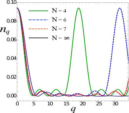
Figure 1: Excitation number $n_{q}$ versus $q$ for $N=4,\,6,\,7$ and $\infty$ quenches at times $t_{n}=nT/(N-1)$ with $K_{n}=1-0.35n/N$ and $T=1$. Momentum $q$ is in units of $1/a$ and time in units of $a/v$.

II.2 The equal-time propagator

The equal-time one-particle propagator is defined as

$$G^{[N]}(x,t)=\langle\Psi_{0}(t)|\psi_{R}(x)\psi^{{\dagger}}_{R}(0)|\Psi_{0}(t)\rangle,$$ (8)

where the superscript $N$ specifies the number of sudden quenches of the switching protocol. To calculate $G^{[N]}$ we express the fermion fields in terms of the boson fields, expand the latter in elementary excitations and exploit the transformations (6) between two consecutive $b$ operators. We then obtain

$$G^{[N]}(x,t)=\frac{1}{2\pi a}e^{\sum_{q>0}e^{-aq}\frac{\pi}{\mathcal{L}q}\left(2i\sin qx-|F_{Rq,0}|^{2}-|F_{Lq,0}|^{2}\right)},$$ (9)

where the functions $F_{\alpha q,0}(x,t)$ are solutions of the recursive relations

$$F_{\alpha q,n}=F_{\alpha q,n+1}e^{-ivq\Delta t_{n}}c_{n}-F_{\bar{\alpha}q,n+1}^{\ast}e^{ivq\Delta t_{n}}s_{n},$$ (10)

with boundary conditions $F_{Rq,N}=(e^{iqx}-1)\cosh\varphi_{N}$, $F_{Lq,N}=(e^{-iqx}-1)\sinh\varphi_{N}$. Like in Eq. (LABEL:recrelexe) the general recursive scheme is obtain by replacing $vt_{n}\to v_{n}t_{n}$.

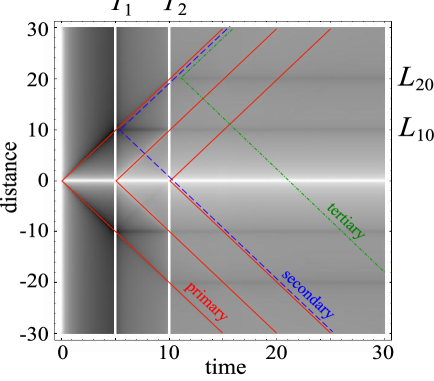
Figure 2: Density plot of $\ln|G^{[N]}(x,t)|$ (arbitrary units) for $N=3$ as a function of time and distance. The parameters are $K_{0}=1,\,K_{1}=0.1,\,K_{2}=0.5,\,K_{3}=0.9$ and $T_{0}=0,\,T_{1}=5,\,T_{2}=10$. Time is in units of $10a/v$ and distance is in units of $10a$.

The full analytic expression of $G^{[N]}$ grows in complexity with increasing $N$. To illustrate the typical features of $G^{[N]}$ in Fig. 2 we report the contour plot of $\ln|G^{[N]}(x,t)|$ for $N=3$. The propagator has a Fermi liquid exponent in the light-cone region $t<x/2v$, in agreement with Refs. cazalilla, ; cardy, . At the quenching times $t_{n}$ the propagator exhibits a time-derivative discontinuity due to the sudden change of the interaction which, being a global perturbation, instantaneously affects the whole system. The $n$-th quench gives rise to incoherent excitations that propagate at a speed $v$ and those at distance $x$ scatter at time $t=t_{n}+x/2v$. When $x=L_{mn}=2v(t_{m}-t_{n})$ the scattering time coincides with the time of the $m$-th quench and a pronounced peak in $\ln|G^{[N]}(x,t)|$ as a function of $x$ develops and persists forever. The peaks are visible as horizontal lines in the contour plot at $x=L_{10}=L_{21}$ and $L_{20}$. Besides the primary light-cone patterns with origin in $x=0$ and $t=t_{n}$ we can see secondary light-cone patterns with origin in $x=L_{mn}$ and $t=t_{m}$ which in turn generate ternary light-cone patterns and so on and so forth in a cascade that grows like $2^{N}$.

In Fig. 3 we display the steady-state value $\lim_{t\to\infty}G^{[3]}(x,t)$ with spikes at the characteristic length scales $L_{mn}$, in accordance with our previous discussion. The analytic expression of $\lim_{t\to\infty}G^{[N]}(x,t)$ is not a simple power-law. Nevertheless, a power-law behavior $\sim x^{-\beta}$ is recovered at short and long distances (see inset of Fig. 3). By employing the recursive method of Eq. (10) we found for the steady-state behavior of $G^{[N]}$ at short distances

$$\lim_{x\to 0}\lim_{t\to\infty}G^{[N]}(x,t)\approx\frac{i}{2\pi(x+ia)}\left|\frac{a}{x}\right|^{\beta_{\rm sd}[K_{n}]},$$ (11)

with a history and initial-state dependent (through $K_{0}$) exponent

$$\beta_{\rm sd}[K_{n}]=\frac{1+K_{N}^{2}}{2K_{0}}\prod_{n=1}^{N}\frac{1}{2}\left[1+\left(\frac{K_{n-1}}{K_{n}}\right)^{2}\right]-1.$$ (12)

The product structure of this result is similar to that of the exponent $\beta$ in the I-V characteristic $I\propto V^{\beta}$ of an out-of-equilibrium LL subject to a sequence of interaction quenches.perfetto Note that $\beta_{\rm sd}$ only depends on the interaction parameters $K_{n}$ and not on the switching times $t_{n}$.nota2 Equation (12) returns the well-known exponent of a LL in the ground state for $K_{0}=K_{1}\ldots=K_{N}\equiv K$ since $\beta_{\rm sd}=(K+1/K)/2-1$, and the exponent of a LL after a single interaction quench for $K_{0}=K_{1}=\ldots=K_{n}=1$ and $K_{n+1}=\ldots=K_{N}=K$ since $\beta_{\rm sd}=(1+K^{2})^{2}/(4K^{2})-1$, in agreement with Ref. cazalilla, .

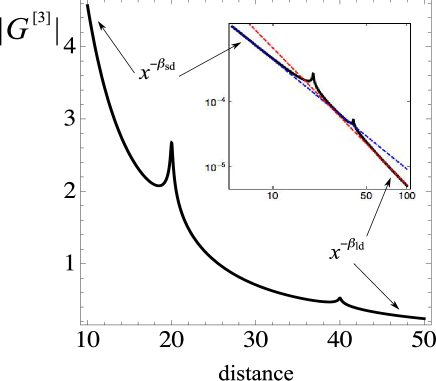
Figure 3: Steady-state value of $|G^{[3]}|$ versus $x$ for $K_{0}=1,\,K_{1}=0.8,\,K_{2}=0.6,\,K_{3}=0.4$ and $T_{0}=0,\,T_{1}=10,\,T_{2}=20$. The crossover between the short and long distance regimes is clearly visible in the inset. Distance is in units of $10a$ and $G^{[3]}$ is in units of $10^{-4}/2\pi a$.

The situation is radically different at long distances. In this limit the dependence on $x$ of the steady-state propagator is again a power-law

$$\lim_{x\to\infty}\lim_{t\to\infty}G^{[N]}(x,t)\approx\frac{i}{2\pi(x+ia)}\left|\frac{R[t_{n},K_{n}]}{x}\right|^{\beta_{\rm ld}[K_{n}]},$$ (13)

but $R[t_{n},K_{n}]$ is a length depending on all intermediate switching times $t_{n}$ and interactions $K_{n}$. As for the exponent $\beta_{\rm ld}$ a striking cancellation of the intermediate $K_{n}$ occurs and we find

$$\beta_{\rm ld}[K_{n}]=\frac{(K_{0}^{2}+K_{N}^{2})(1+K_{N}^{2})}{4K_{0}K_{N}^{2}}-1,$$ (14)

which depends only on the initial state.

To summarize the steady-state propagator does not thermalize for discontinuous switchings, and the thermalization breakdown manifests in different ways at short and long distances. In the next Section we address the evolution of this behavior when the sequential protocol approaches a continuous protocol.

III Continuous quenches

Continuous switching protocols are obtained as a limiting case of a sequential quench. Let us start by analyzing again the excitation energy $\Delta E(t)$. Taking the quenching times $t_{n}=nt/(N-1)$ equally spaced and letting $N\to\infty$ the variable $t_{n}$ becomes a continuous variable between $0$ and $t$ and we can construct the differentiable functions $P_{q}(s)$, $Q_{q}(s)$ and $\varphi(s)$ according to $P_{q}(t_{n})=P_{q,n}$, $Q_{q}(t_{n})=Q_{q,n}$ and $\varphi(t_{n})=\varphi_{n}$. Expanding Eqs. (LABEL:recrelexe) to first order in $\Delta t_{n}=\Delta t=t/(N-1)$ and $\Delta\varphi_{n}$ we find a coupled system of differential equations

$$\frac{dP_{q}}{ds} = -2\mathrm{Re}[Q_{q}]\frac{d\varphi}{ds},$$

$$\frac{dQ_{q}}{ds} = -2P_{q}\frac{d\varphi}{ds}+2ivqQ_{q},$$ (15)

that should be solved with boundary conditions $P_{q}(t)=1$ and $Q_{q}(t)=0$. The average occupation number $n_{q}(t)$ is then simply given by $1-P_{q}(0)$. The most popular continuous protocol is the ramp-switchingtanteramps $\varphi(s)=\bar{\varphi}s/t$ with $0<s<t$. In this case the system (15) can be solved exactly and we find

$$n_{q}(t)=\frac{\bar{\varphi}t}{v}\times\frac{1-\cos[\frac{2v}{t}\sqrt{q^{2}-(\frac{\bar{\varphi}t}{v})^{2}}]}{q^{2}-(\frac{\bar{\varphi}t}{v})^{2}},$$ (16)

which correctly approaches zero for $t\to\infty$ (adiabatic limit), whereas for any finite $t$ is exponentially suppressed at large $q$, see the curve $N\to\infty$ in Fig. 1. We also checked that inserting Eq. (16) into Eq. (5) and taking the long-time limit $t\to\infty$ and the weak-coupling limit $\bar{\varphi}\ll va/t$ the excitation energy vanishes as

$$\lim_{t\to\infty}\Delta E(t)\sim\mathcal{L}\frac{\ln t}{t^{2}},\quad\quad\bar{\varphi}\ll va/t,$$ (17)

in agreement with Ref. dhz.2010, . It is interesting to observe that the dependence of $\Delta E\sim\delta^{2}\ln\delta$ on the ramp rate $\delta=\bar{\varphi}/t$ is not a simple power-law $\delta^{\nu}$ and, therefore, does not belong to the non-analytic regimes contemplated in Ref. ramp, .

The system of differential equations (15) is exact (non-perturbative) and we now exploit it to prove that there exist no switching protocol of finite duration capable to drive the initial non-interacting system in the interacting ground state of a LL. Since $\Delta E(t)$ is the sum of non-negative $n_{q}$’s it is sufficient to show that $n_{0}(t)=1-P_{0}(0)$ cannot be zero. The optimal switching protocol $\varphi(s)$ that reproduces a target $P_{0}(s)$ follows from Eqs. (15) with $q=0$; in this case $\varphi(s)$ depends only on the instantaneous value of $P_{0}(s)$, and reads

$$\varphi(s)=\bar{\varphi}-\frac{1}{2}\cosh^{-1}P_{0}(s),$$ (18)

where $\bar{\varphi}$ is the value of the correlation angle at the end of the quench. Thus, $P_{0}(0)=1$ only provided that the initial and final strength of the interaction is the same, $\varphi(0)=\bar{\varphi}$. In particular $n_{0}(t)>0$ for all switching protocols that connect an initial interaction strength $K_{0}$ to a final interaction strength $K\neq K_{0}$.

Analytic results can be obtained for the one-particle propagator as well. Let us start by analyzing the exponents $\beta$ of the long- and short-distance power-law behavior of $G^{[N]}$. For a continuous switching we can construct the differentiable function $K(s)$ according to $K(t_{n})=K_{n}$, with $K(0)=K_{0}$ and $K(t)=K$. Approximating $K(t_{n-1})=K(t_{n}-\frac{T}{N})\approx K(t_{n})-\frac{T}{N}K^{\prime}(t_{n})$ and taking the logarithm of Eq. (12) we find

$$\ln\left[\frac{2K_{0}(\beta_{\rm sd}+1)}{1+K^{2}}\right] = \lim_{N\to\infty}\sum_{n=1}^{N}\log\left[1-\frac{T}{N}\frac{K^{\prime}(t_{n})}{K(t_{n})}\right]$$

$$= -\int_{0}^{t}ds\frac{K^{\prime}(s)}{K(s)}=\ln\frac{K_{0}}{K},$$

and hence

$$\beta_{\rm sd}[K(s)]=\frac{1}{2}\left(K+\frac{1}{K}\right)-1,$$ (19)

which coincides with the exponent of a ground-state LL. Therefore, at short distances the initial-state dependence as well as the history dependence are washed out by differentiable switchings and the propagator thermalizes. Discontinuous switchingsnota do, instead, introduce a history dependence through the ratio between the values of $K(s)$ across the discontinuity. To the contrary the long-distance exponent $\beta_{\rm ld}$ in Eq. (14) is always history independent and the steady-state propagator does never thermalize. Our conclusions agree with recent perturbative results by Dòra et al. in Ref. dhz.2010, .

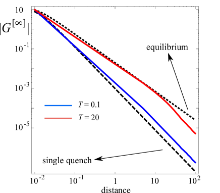
Figure 4: Steady-state propagator $|G^{[\infty]}|$ versus $x$ for two different ramp switching-times (in units of $10^{2}a/v$) $T=0.1$ (blue solid) and $T=20$ (red solid) and $\bar{\varphi}=0.46$. For comparison the equilibrium propagator with exponent $\beta_{\rm{sd}}$ (dotted) and the sudden quench propagator with exponent $\beta_{\rm{ld}}$ (dashed) are also shown. Distances are in units of $10^{2}a$ and $|G^{[\infty]}|$ is in units of $10^{-2}/a$.

To study the crossover from short to long distances we must calculate the steady-state propagator at all $x$. For continuous switching the recursive system of Eq. (10) reduces to a system of differential equations

$$\frac{d}{ds}F_{\alpha q}=ivqF_{\alpha q}+F^{*}_{\bar{\alpha}q}\frac{d\varphi}{ds},$$ (20)

that should be solved with boundary conditions $F_{Rq}(t)=(e^{iqx}-1)\cosh\varphi(t)$ and $F_{Lq}(t)=(e^{-iqx}-1)\sinh\varphi(t)$. The equal-time propagator $G^{[\infty]}(x,t)$ can then be calculated from Eq. (9) with $F_{\alpha q,0}=F_{\alpha q}(0)$. In the special case of a ramp protocol $\varphi(s)=\bar{\varphi}s/T$ for $s<T$ and $\varphi(s)=\bar{\varphi}$ for $T<s<t$ the system of equations (20) can be solved analytically and we get

$$F_{Rq}(0)\!\! = \!\!\frac{(1-e^{iqx})\sinh\gamma_{q}}{\gamma_{q}}[e^{ivq(t-T)}\bar{\varphi}\sinh\bar{\varphi}$$ (21)

$$+ \!\!e^{-ivq(t-T)}(iqvT-\gamma_{q}\frac{e^{2\gamma_{q}}+1}{e^{2\gamma_{q}}-1})\cosh\bar{\varphi}],$$

where $\gamma_{q}=\sqrt{\bar{\varphi}^{2}-(vqT)^{2}}$; the function $F^{*}_{Lq}(0)$ is obtained from $F_{Rq}(0)$ simply by exchanging $\sinh\bar{\varphi}\leftrightarrow\cosh\bar{\varphi}$ and by replacing $v\to-v$. In Fig. 4 we plot the steady-state propagator $|G^{[\infty]}|$ as a function of the distance $x$ for two different ramp switching-times and $\bar{\varphi}=0.46$, which corresponds to the LL parameter $K=0.4$. The results clearly agree with the scenario outlined above: at distances smaller than the characteristic length $2vT$ the steady-state propagator behaves thermally while at large distances it behaves like the sudden-quench (nonthermal) propagator of Ref. cazalilla, , albeit shifted upwards by a history-dependent constant (see also Ref. dhz.2010, ).

The long-to-short distance crossover is particularly transparent in the weak coupling limit $\bar{\varphi}\ll 1$. In this case we can expand $F_{\alpha q}(0)$ to second order in $\bar{\varphi}$, perform the sum over $q$ and find the steady-state propagator $G^{[\infty]}$ at all $x$

$$\lim_{t\to\infty}G^{[\infty]}(x,t) \approx \frac{i}{2\pi(x+ia)}\left|\frac{a^{2}}{x^{2}-(2vT)^{2}}\right|^{\bar{\varphi}^{2}}\left|\frac{2vT}{x}\right|^{2\bar{\varphi}^{2}}$$ (22)

$$\times \left|\frac{x^{2}}{x^{2}-(2vT)^{2}}\right|^{\frac{x^{2}\bar{\varphi}^{2}}{4v^{2}T^{2}}}\left|\frac{x-2vT}{x+2vT}\right|^{\frac{x\bar{\varphi}^{2}}{v}}\!\!\!\!,$$

with power-law exponents depending on $x$. Equation (22) reproduces with remarkable accuracy the long-to-short distance crossover, which in the same approximation read

$$\lim_{x\to 0}\lim_{t\to\infty}G^{[\infty]}(x,t) \approx \frac{i}{2\pi(x+ia)}\left|\frac{a}{x}\right|^{2\bar{\varphi}^{2}},$$ (23)

$$\lim_{x\to\infty}\lim_{t\to\infty}G^{[\infty]}(x,t) \approx \frac{i}{2\pi(x+ia)}\left|\frac{R}{x}\right|^{4\bar{\varphi}^{2}},$$ (24)

$R=\sqrt{2vTa}$ being a history-dependent length [cfr. Eq.(13)]. The high accuracy stems from the fact that the correlation angle $\varphi$ remains small also in the intermediate coupling regime characterized by $g_{2}\approx g_{4}\approx v_{F}$ for which $\varphi\approx 0.1$.

Finally we observe that from Fig. 4 and Eq. (22) the adiabatic limit is recovered when the switching time $T\to\infty$. As $T$ increases the steady-state propagator equals the equilibrium propagator up to larger and larger values of $x$.

IV Conclusions

We provided a comprehensive analysis of the relaxation dynamics of a LL after the quenching of the electron-electron interaction for different switching protocols. The bosonization method is combined with a recursive procedure to address arbitrary sequences of sudden quenches and hence, as a limiting case, continuous protocols. The approach allows us to evaluate the excitation energy $\Delta E$ and the equal-time one-particle propagator $G$. We found that for a sequence of sudden quenches $\Delta E$ is always larger than zero. The thermalization breakdown has a dramatic impact on the propagator both at finite times and at the steady-state. In particular the steady-state $G$ exhibits a power-law behavior $|x|^{-\beta}$ with different exponents at long and short distances. Remarkable we are able to express $\beta$ as explicit functionals of the switching protocol. We found that at long distances $\beta=\beta_{\rm ld}$ carries informations on the initial state but not on the history of the switching protocol, and coincides with the exponent of a sudden quench.cazalilla At short distances $\beta=\beta_{\rm sd}$ is, instead, both initial-state and history dependent; it is only for continuous protocols that memory is washed out and $\beta_{\rm sd}$ equals the exponent of a LL in equilibrium.

The continuous limit of the recursive procedure leads to a simple system of differential equations that can be solved numerically. For the excitation energy $\Delta E$ we proved that there exist no switching protocols of finite duration capable to bring a system from a non-interacting ground-state to the ground state of a LL. It is only in the adiabatic limit that thermalization occurs. These results may be relevant to design the optimal switching protocol that minimizes the total excitation energy or the energy a of given $q$-excitation. For the propagator $G$ we clarify how the adiabatic limit is attained by studying ramp-switching protocols of increasing duration $T$. At weak coupling we derive an explicit expression for $G(x,t\to\infty)$ that is valid for all $x$ and around the crossover distance $x\approx 2vT$ is dominated by a power-law $|x-2vT|^{-\beta(x)}$ with a $x$-dependent exponent. The formula further reproduces with remarkable accuracy the different power-laws at long and short distances. Our predictions could be experimentally confirmed by measurements in ultracold fermionic atoms loaded in optical lattices, recently proposedllopt1 ; llopt2 as candidates to realize highly controllable and tunable LLs.

References

- (1) T. Kinoshita, T. Wenger, and D. S. Weiss, Nature 440, 900 (2006).
- (2) I. Bloch, J. Dalibard, and W. Zwerger, Rev. Mod. Phys. 80, 885 (2008).
- (3) M. Greiner, O. Mandel, T. Esslinger, T. W. Hänsch, and I. Bloch, Nature 415, 39 (2002).
- (4) T. Stöferle, H. Moritz, C. Schori, M. Köhl, and T. Esslinger, Phys. Rev. Lett. 92, 130403 (2004).
- (5) K. Winkler, G. Thalhammer, F. Lang, R. Grimm, J. Hecker Denschlag, A. J. Daley, A. Kantian, H. P. Büchler, and P. Zoller, Nature 441, 853 (2006).
- (6) I. B. Spielman, W. D. Phillips, and J. V. Porto, Phys. Rev. Lett. 98, 080404 (2007).
- (7) M. Köhl, H. Moritz, T. Stöferle, K. Günter, and T. Esslinger, Phys. Rev. Lett. 94, 080403 (2005).
- (8) R. Jördens, N. Strohmaier, K. Günter, H. Moritz, and T. Esslinger, Nature 455, 204 (2008).
- (9) U. Schneider, L. Hackermüller, S. Will, T. Best, I. Bloch, T. A. Costi, R. W. Helmes, D. Rasch, and A. Rosch, Science 322, 1520 (2008).
- (10) C. Kollath, A. M. Läuchli, and E. Altman, Phys. Rev. Lett. 98, 180601 (2007).
- (11) S.R. Manmana, S. Wessel, R. M. Noack, and A. Muramatsu, Phys. Rev. Lett. 98, 210405 (2007).
- (12) M. Rigol, Phys. Rev. Lett. 103, 100403 (2009).
- (13) T. Barthel and U. Schollwöck, Phys. Rev. Lett. 100, 100601 (2008).
- (14) G. Stefanucci and C-O Almbladh, Phys. Rev. B 69 195318 (2004); Eur. Phys. Lett. 67 14 (2004).
- (15) G. Stefanucci, Phys. Rev. B 75, 195115 (2007).
- (16) H. D. Cornean et al., Ann. H Poincarè 10, 61 (2009).
- (17) M Rigol, V. Dunjko, V. Yurovsky, and M. Olshanii, Phys. Rev. Lett. 98, 050405 (2007).
- (18) J. Werschnik and E. K. U. Gross, J. Phys. B: At. Mol. Opt. Phys. 40, R175 (2007).
- (19) C. Brif, R. Chakrabarti and H. Rabitz, New J. Phys. 12, 075008 (2010).
- (20) A. Rahmani and C. Chamon, arXiv:1011.3061v2
- (21) M. A. Cazalilla, Phys. Rev. Lett. 97, 156403 (2006).
- (22) E. Perfetto, G. Stefanucci and M. Cini, Phys. Rev. Lett. 105, 156802 (2010).
- (23) E. Perfetto, Phys. Rev. B. 74,205123 (2006).
- (24) A. Iucci and M. A. Cazalilla, Phys. Rev. A. 80, 063619 (2009).
- (25) G. S. Uhrig, Phys. Rev. A 80, 061602(R) (2009).
- (26) Zhou Zong-Li and Lou Ping, Commun. Theor. Phys. 51 1139 (2009).
- (27) Zhou Zong-Li, Zhang Guo-Shun and Lou Ping, Chinese Phys. Lett. 27, 067305 (2010).
- (28) B. Dóra, M. Haque and G. Zaránd, arXiv:1011.6655v1.
- (29) T. Giamarchi, Quantum Physics in One Dimension (Clarendon, Oxford, 2004).
- (30) P. Calabrese and J. Cardy, Phys. Rev. Lett. 96, 136801 (2006).
- (31) It is possible to show that the critical exponents and are independent of the value of the renormalized velocities .
- (32) For memory effects to be detectable it is enough that changes on a time scale faster than .
- (33) M. Eckstein and M. Kollar, New J. Phys. 12, 055012, (2010); T. Hikichi, S. Suzuki, and K. Sengupta, Phys. Rev. B 82, 174305 (2010); T. Venumadhav, M. Haque, R. Moessner, Phys. Rev. B 81, 054305 (2010).
- (34) A. Polkovnikov and V. Gritsev, Nature Physics 4, 477 (2008).
- (35) K. Günter, T. Stöferle, H. Moritz, M. Köhl and T. Esslinger, Phys. Rev. Lett. 95, 230401 (2005).
- (36) P. Pedri, S. De Palo, E. Orignac, R. Citro and M. L. Chiofalo, Phys. Rev. A 77, 015601 (2008).