Minimizing the sum of many rational functions

Abstract

We consider the problem of globally minimizing the sum of many rational functions over a given compact semialgebraic set. The number of terms can be large (10 to 100), the degree of each term should be small (up to 10), and the number of variables can be large (10 to 100) provided some kind of sparsity is present. We describe a formulation of the rational optimization problem as a generalized moment problem and its hierarchy of convex semidefinite relaxations. Under some conditions we prove that the sequence of optimal values converges to the globally optimal value. We show how public-domain software can be used to model and solve such problems.

Keywords: rational optimization; global optimization; semidefinite relaxations; sparsity.
AMS MSC 2010: 46N10, 65K05, 90C22, 90C26.

1 Introduction

Consider the optimization problem

$$f^{*}\,:=\,\displaystyle\inf_{\mathbf{x}\in\mathbf{K}}\>\sum_{i=1}^{N}f_{i}(\mathbf{x})$$ (1)

over the basic semi-algebraic set

$$\mathbf{K}\,:=\,\{\mathbf{x}\in\mathbb{R}^{n}\>:\>g_{j}(\mathbf{x})\,\geq\,0,\>j=1,\ldots,m\>\},$$ (2)

for given polynomials $g_{j}\in\mathbb{R}[\mathbf{x}]$, $j=1,\ldots,m$, and where each term $f_{i}:\mathbb{R}^{n}\to\mathbb{R}$ is a rational function

$$\mathbf{x}\mapsto f_{i}(\mathbf{x}):=\frac{p_{i}(\mathbf{x})}{q_{i}(\mathbf{x})},$$

with $p_{i},q_{i}\in\mathbb{R}[\mathbf{x}]$ and $q_{i}>0$ on $\mathbf{K}$, for each $i=1,\ldots,N$.

Problem (1) is a fractional programming problem of a rather general form. Nevertheless, we assume that the degree of each $f_{i}$ and $g_{j}$ is relatively small (up to 10), but the number of terms $N$ can be quite large (10 to 100). For dense data the number of variables $n$ should also be small (up to 10). However, this number can be also quite large (10 to 100) provided that the problem data feature some kind of sparsity (to be specified later). Even though problem (1) is of self-interest, our initial motivation came from some applications in computer vision, where such problems are typical. These applications will be described elsewhere.

In such a situation, fractional programming problem (1) is quite challenging. Indeed, we make no assumption on the polynomials $p_{i},q_{i}$ whereas even with a relatively small number of fractions and under convexity (resp. concavity) assumptions on $p_{i}$ (resp. $q_{i}$), problem (1) is hard to solve (especially if one wants to compute the global minimum); see for example the survey [10] and references therein.

We are interested in solving problem (1) globally, in the sense that we do not content ourselves with a local optimum satisfying first order optimality conditions, as typically obtained with standard local optimization algorithms such as Newton’s method or its variants. If problem (1) is too difficult to solve globally (because of ill-conditioning and/or too large a number of variables or terms in the objective function), we would like to have at least a valid lower bound on the global minimum, since upper bounds can be obtained with local optimization algorithms.

One possible approach is to reduce all fractions $p_{i}/q_{i}$ to same denominator and obtain a single rational fraction to minimize. Then one may try to apply the hierarchy of semidefinite programming (SDP) relaxations defined in [6], see also [9, Section 5.8]. But such a strategy is not appropriate because the degree of the common denominator is potentially large and even if $n$ is small, one may not even implement the first relaxation of the hierarchy, due to the present limitations of SDP solvers. Moreover, in general this strategy also destroys potential sparsity patterns present in the original formulation (1), and so precludes from using an appropriate version (for the rational fraction case) of the sparse semidefinite relaxations introduced in [11] whose convergence was proved in [7] under some conditions on the sparsity pattern, see also [9, Sections 4.6 and 5.3.4].

Another possibility is to introduce additional variables $r_{i}$ (that we may call liftings) with associated constraints

$$\frac{p_{i}(\mathbf{x})}{q_{i}(\mathbf{x})}\leq r_{i},\>i=1,\ldots,N,$$

and solve the equivalent problem:

$$f^{*}\,:=\,\displaystyle\inf_{(\mathbf{x},\mathbf{r})\in\widehat{\mathbf{K}}}\>\sum_{i=1}^{N}r_{i}$$ (3)

which is now a polynomial optimization problem in the new variables $(\mathbf{x},\mathbf{r})\in\mathbb{R}^{n}\times\mathbb{R}^{N}$, and where the new feasible set $\widehat{\mathbf{K}}=\mathbf{K}\times\{(\mathbf{x},\mathbf{r})\in\mathbb{R}^{n+N}\>:\>r_{i}q_{i}(\mathbf{x})-p_{i}(\mathbf{x})\geq 0\}$ is modeling the epigraphs of the rational terms. The sparsity pattern is preserved and if $\mathbf{K}$ is compact one may in general obtain upper and lower bounds $\overline{r}_{i},\underline{r}_{i}$ on the $r_{i}$ so as to make $\widehat{\mathbf{K}}$ compact by adding the quadratic (redundant) constraints $(r_{i}-\underline{r}_{i})(\overline{r}_{i}-r_{i})\geq 0$, $i=1,\ldots,N$, and apply the sparse semidefinite relaxations. However, in doing so one introduces $N$ additional variables, and this may have an impact on the overall performance, especially if $N$ is large. In the sequel this approach is referred to as the epigraph approach.

The goal of the present paper is to circumvent all above difficulties in the following two situations: either $n$ is relatively small, or $n$ is potentially large but some sparsity is present, i.e., each $f_{i}$ and each $g_{j}$ in (1) is concerned with only a small subset of variables. In the approach that we propose, we do not need the epigraph liftings. The idea is to formulate (1) as an equivalent infinite-dimensional linear problem which a particular instance of the generalized moment problem (GMP) as defined in [8], with $N$ unknown measures (where each measure is associated with a fraction $p_{i}/q_{i}$). In turn this problem can be easily modeled and solved with our public-domain software GloptiPoly 3 [5], a significant update of GloptiPoly 2 [4]. In the sequel this approach is referred to as the GMP approach.

The outline of the paper is as follows. In Section 2 we introduce the SDP relaxations first in the case that $n$ is small and the data are dense polynomials. Then in Section 3 we extend the SDP relaxations to the case that $n$ is large but sparsity is present. In Section 4 we show how the GMP formulation can be exploited to model the SDP relaxations of problem (1) easily with GloptiPoly 3. We also provide a collection of numerical experiments showing the relevance of our GMP approach, especially in comparison with the epigraph approach.

2 Dense SDP relaxations

In this section we assume that $n$, the number of variables in problem (1), is small, say up to 10.

2.1 GMP formulation

Consider the infinite dimensional linear problem

$$\begin{array}[]{rl}\hat{f}\,:=\,\displaystyle\inf_{\mu_{i}\in\mathcal{M}(\mathbf{K})}&\displaystyle\sum_{i=1}^{N}\int_{\mathbf{K}}p_{i}\,d\mu_{i}\\ \mbox{s.t.}&\displaystyle\int_{\mathbf{K}}q_{1}d\mu_{1}=1\\ &\\ &\displaystyle\int_{\mathbf{K}}\mathbf{x}^{\mathbf{\alpha}}q_{i}d\mu_{i}=\displaystyle\int_{\mathbf{K}}\mathbf{x}^{\mathbf{\alpha}}q_{1}d\mu_{1},\quad\forall\mathbf{\alpha}\in\mathbb{N}^{n},\>i=2,\ldots,N,\end{array}$$ (4)

where $\mathcal{M}(\mathbf{K})$ is the space of finite Borel measures supported on $\mathbf{K}$.

Theorem 2.1

Let $\mathbf{K}\subset\mathbb{R}^{n}$ in (2) be compact, and assume that $q_{i}>0$ on $\mathbf{K}$, $i=1,\ldots,N$. Then $\hat{f}=f^{*}$.

Proof: We first prove that $f^{*}\geq\hat{f}$. As $f=\sum_{i}p_{i}/q_{i}$ is continuous on $\mathbf{K}$, there exists a global minimizer $\mathbf{x}^{*}\in\mathbf{K}$ with $f(\mathbf{x}^{*})=f^{*}$. Define $\mu_{i}:=q_{i}(\mathbf{x}^{*})^{-1}\delta_{\mathbf{x}^{*}}$, $i=1,\ldots,N$, where $\delta_{\mathbf{x}^{*}}$ is the Dirac measure at $\mathbf{x}^{*}$. Then obviously, the measures $(\mu_{i})$, $i=1,\ldots,N$, are feasible for (4) with associated value

$$\sum_{i=1}^{N}\int_{\mathbf{K}}p_{i}d\mu_{i}\,=\,\sum_{i=1}^{N}p_{i}(\mathbf{x}^{*})/q_{i}(\mathbf{x}^{*})=f(\mathbf{x}^{*})=f^{*}.$$

Conversely, let $(\mu_{i})$ be a feasible solution of (4). For every $i=1,\ldots,N$, let $d\nu_{i}$ be the measure $q_{i}d\mu_{i}$, i.e.

$$\nu_{i}(B):=\int_{\mathbf{K}\cap B}q_{i}(\mathbf{x})d\mu_{i}(\mathbf{x})$$

for all sets $B$ in the Borel $\sigma$-algebra of $\mathbb{R}^{n}$, and so the support of $\nu_{i}$ is $\mathbf{K}$. As measures on compact sets are moment determinate, the moments constraints of (4) imply that $\nu_{i}=\nu_{1}$, for every $i=2,\ldots,N$, and from $\int_{\mathbf{K}}q_{1}d\mu_{1}=1$ we also deduce that $\nu_{1}$ is a probability measure on $\mathbf{K}$. But then

$$\sum_{i=1}^{N}\int_{\mathbf{K}}p_{i}d\mu_{i} = \sum_{i=1}^{N}\int_{\mathbf{K}}\frac{p_{i}}{q_{i}}q_{i}d\mu_{i}=\sum_{i=1}^{N}\int_{\mathbf{K}}\frac{p_{i}}{q_{i}}d\nu_{1}$$

$$= \int_{\mathbf{K}}\left(\sum_{i=1}^{N}\frac{p_{i}}{q_{i}}\right)\,d\nu_{1}\,=\,\int_{\mathbf{K}}fd\nu_{1}\geq\int_{\mathbf{K}}f^{*}d\nu_{1}\,=\,f^{*},$$

where we have used that $f\geq f^{*}$ on $\mathbf{K}$ and $\nu_{1}$ is a probability measure on $\mathbf{K}$. $\Box$

We next make the following assumption meaning that set $\mathbf{K}$ admits an algebraic certificate of compactness.

Assumption 2.1

The set $\mathbf{K}\subset\mathbb{R}^{n}$ in (2) is compact and the quadratic polynomial $\mathbf{x}\mapsto M-\|\mathbf{x}\|^{2}$ can be written as

$$M-\|\mathbf{x}\|^{2}=\sigma_{0}+\sum_{j=1}^{m}\sigma_{j}\,g_{j},$$

for some polynomials $\sigma_{j}\in\mathbb{R}[\mathbf{x}]$, all sums of squares of polynomials.

2.2 A hierarchy of dense SDP relaxations

Let $\mathbf{y}_{i}=(y_{i\mathbf{\alpha}})$ be a real sequence indexed in the canonical basis $(\mathbf{x}^{\mathbf{\alpha}})$ of $\mathbb{R}[\mathbf{x}]$, $i=1,\ldots,N$, and for every $k\in\mathbb{N}$, let $\mathbb{N}^{n}_{k}:=\{\alpha\in\mathbb{N}^{n}:\sum_{j}\alpha_{j}\leq k\}$.

Define the moment matrix $M_{k}(\mathbf{y}_{i})$ of order $k$, associated with $\mathbf{y}$, whose entries indexed by multi-indices $\beta$ (rows) and $\gamma$ (columns) read

$$[M_{k}(\mathbf{y}_{i})]_{\beta,\gamma}:=y_{i(\beta+\gamma)},\quad\forall\,\beta,\,\gamma\in\mathbb{N}^{n}_{k},$$

and so are linear in $\mathbf{y}_{i}$. Similarly, given a polynomial $g(\mathbf{x})=\sum_{\alpha}g_{\alpha}\mathbf{x}^{\alpha}$, define the localising matrix $M_{k}(g\mathbf{y}_{i})$ of order $k$, associated with $\mathbf{y}$ and $g$, whose entries read

$$[M_{k}(g\,\mathbf{y}_{i})]_{\beta,\gamma}:=\sum_{\alpha}g_{\alpha}y_{i(\alpha+\beta+\gamma)},\quad\forall\,\beta,\gamma\in\mathbb{N}^{n}_{k}.$$

In particular, matrix $M_{0}(g\mathbf{y}_{i})$ is identical to $L_{\mathbf{y}_{i}}(g)$ where for every $i$, $L_{\mathbf{y}_{i}}:\mathbb{R}[\mathbf{x}]\to\mathbb{R}$ is the linear functional defined by:

$$g\>\mapsto\>L_{\mathbf{y}_{i}}(g)\,:=\,\sum_{\alpha\in\mathbb{N}^{n}}g_{\alpha}y_{i\alpha},\qquad\forall g\in\mathbb{R}[\mathbf{x}].$$

Let $u_{i}:=\lceil({\rm deg}\,q_{i})/2\rceil$, $i=1,\ldots,N$, $r_{j}:=\lceil({\rm deg}\,g_{j})/2\rceil$, $j=1,\ldots,m$, and with no loss of generality assume that $u_{1}\leq u_{2}\leq\ldots\leq u_{N}$. Consider the hierarchy of semidefinite programming (SDP) relaxations:

$$\begin{array}[]{rll}f^{*}_{k}=\displaystyle\inf_{\mathbf{y}_{i}}&\displaystyle\sum_{i=1}^{N}L_{\mathbf{y}_{i}}(p_{i})&\\ \mbox{s.t.}&M_{k}(\mathbf{y}_{i})\succeq 0,&i=1,\ldots,N\\ &M_{k-r_{j}}(g_{j}\mathbf{y}_{i})\succeq 0,&i=1,\ldots,N,\>j=1,\ldots,m\\ &L_{\mathbf{y}_{1}}(q_{1})\,=\,1\\ &L_{\mathbf{y}_{i}}(\mathbf{x}^{\mathbf{\alpha}}q_{i})=L_{\mathbf{y}_{1}}(\mathbf{x}^{\mathbf{\alpha}}q_{1}),&\forall\mathbf{\alpha}\in\mathbb{N}^{n}_{2(k-u_{i})},\,i=2,\ldots,N.\end{array}$$ (5)

Theorem 2.2

Let Assumption 2.1 hold and consider the hierarchy of SDP relaxations (5). Then it follows that

1. $f^{*}_{k}\uparrow f^{*}$ as $k\to\infty$.

2. Moreover, if $(\mathbf{y}_{i}^{k})$ is an optimal solution of (5), and if

   $${\rm rank}\,M_{k}(\mathbf{y}_{i}^{k})\,=\,{\rm rank}\,M_{k-u_{i}}(\mathbf{y}_{i}^{k})\,=:\,R,\quad i=1,\ldots,N$$

   then $f^{*}_{k}=f^{*}$ and one may extract $R$ global minimizers.

Proof: The proof of (a) is classical. One first prove that if $(\mathbf{y}_{i}^{k})$ is a nearly optimal solution of (5), i.e.

$$f^{*}_{k}\leq\sum_{i=1}^{N}L_{\mathbf{y}_{i}^{k}}(p_{i})\leq f^{*}_{k}+\frac{1}{k},$$

then there exists a subsequence $(k_{\ell})$ and a sequence $\mathbf{y}_{i}$, $i=1,\ldots,N$, such that

$$\lim_{\ell\to\infty}\,y^{k_{\ell}}_{i\mathbf{\alpha}}\,=\,y_{i\mathbf{\alpha}},\quad\forall\mathbf{\alpha}\in\mathbb{N}^{n},i=1,\ldots,N.$$

From this pointwise convergence it easily follows that for every $i=1,\ldots,N$ and $j=1,\ldots,m$,

$$M_{k}(\mathbf{y}_{i})\succeq 0,\>M_{k}(g_{j}\mathbf{y}_{i})\succeq 0,\quad k=0,1,\ldots$$

By Putinar’s theorem [9, Theorem 2.14] this implies that the sequence $\mathbf{y}_{i}$ has a representing measure supported on $\mathbf{K}$, i.e., there exists a finite Borel measure $\mu_{i}$ on $\mathbf{K}$ such that

$$L_{\mathbf{y}_{i}}(f)\,=\,\int_{\mathbf{K}}fd\mu_{i},\qquad\forall\,f\in\mathbb{R}[\mathbf{x}].$$

Moreover, still by pointwise convergence,

$$L_{\mathbf{y}_{i}}(q_{i}\mathbf{x}^{\mathbf{\alpha}})\,=\,\int_{\mathbf{K}}\mathbf{x}^{\mathbf{\alpha}}q_{i}(\mathbf{x})d\mu_{i}\,=\,L_{\mathbf{y}_{1}}(q_{1}\mathbf{x}^{\mathbf{\alpha}})\,=\,\int_{\mathbf{K}}\mathbf{x}^{\mathbf{\alpha}}q_{1}(\mathbf{x})d\mu_{1},\quad\forall\mathbf{\alpha}\in\mathbb{N}^{n}.$$ (6)

Therefore, let $d\nu_{i}:=q_{i}(\mathbf{x})d\mu_{i}$ which is a probability measure supported on $\mathbf{K}$. As $\mathbf{K}$ is compact, by (6), $\nu_{i}=\nu_{1}$ for every $i=1,\ldots,N$. Finally, again by pointwise convergence:

$$f^{*}\geq\lim_{\ell\to\infty}f^{*}_{k_{\ell}} = \lim_{\ell\to\infty}\sum_{i=1}^{N}L_{\mathbf{y}^{k_{\ell}}_{i}}(p_{i})=\sum_{i=1}^{N}\int_{\mathbf{K}}p_{i}d\mu_{i}$$

$$= \sum_{i=1}^{N}\int_{\mathbf{K}}\frac{p_{i}}{q_{i}}q_{i}d\mu_{i}=\sum_{i=1}^{N}\int_{\mathbf{K}}\frac{p_{i}}{q_{i}}d\nu_{1}$$

$$= \int_{\mathbf{K}}\left(\sum_{i=1}^{N}\frac{p_{i}}{q_{i}}\right)d\nu_{1}\geq f^{*}$$

which proves (a) because $f^{*}_{k}$ is monotone non-decreasing. In addition, $\nu_{1}$ is an optimal solution of (4) with optimal value $f^{*}=\hat{f}$.

Statement (b) follows from the flat extension theorem of Curto and Fialkow [9, Theorem 3.7] and each $\mathbf{y}_{i}$ has an atomic representing measure supported on $R$ points of $\mathbf{K}$. $\Box$

3 Sparse SDP relaxations

In this section we assume that $n$, the number of variables in problem (1), is large, say from 10 to 100, and moreover that some sparsity pattern is present in the polynomial data.

3.1 GMP formulation

Let $I_{0}:=\{1,\ldots,n\}=\cup_{i=1}^{N}I_{i}$ with possible overlaps, and let $\mathbb{R}[x_{k}:k\in I_{i}]$ denote the ring of polynomials in the variables $x_{k},\>k\in I_{i}$. Denote by $n_{i}$ the cardinality of $I_{i}$.

One will assume that $\mathbf{K}\subset\mathbb{R}^{n}$ in (2) is compact, and one knows some $M>0$ such that $\mathbf{x}\in\mathbf{K}\Rightarrow M-\|\mathbf{x}\|^{2}\geq 0$. For every $i\leq N$, introduce the quadratic polynomial $\mathbf{x}\mapsto g_{m+i}(\mathbf{x})=M-\sum_{k\in I_{i}}x_{k}^{2}$. The index set $\{1,\ldots,m+N\}$ has a partition $\cup_{i=1}^{N}J_{i}$ with $J_{i}\neq\emptyset$ for every $i=1,\ldots,N$. In the sequel we assume that for every $i=1,\ldots,N$, $p_{i},q_{i}\in\mathbb{R}[x_{k}:k\in I_{i}]$ and for every $j\in J_{i}$, $g_{j}\in\mathbb{R}[x_{k}:k\in I_{i}]$. Next, for every $i=1,\ldots,N$, let

$$\mathbf{K}_{i}\,:=\,\{\mathbf{z}\in\mathbb{R}^{n_{i}}\>:\>g_{k}(\mathbf{z})\geq 0,\>k\in J_{i}\}$$

so that $\mathbf{K}$ in (2) has the equivalent characterization

$$\mathbf{K}\,=\,\{\mathbf{x}\in\mathbb{R}^{n}\>:\>(x_{k},k\in I_{i})\in\mathbf{K}_{i},\>i=1,\ldots,N\}.$$

Similarly, for every $i,j\in\{1,\ldots,N\}$ such that $i\neq j$ and $I_{i}\cap I_{j}\neq\emptyset$,

$$\mathbf{K}_{ij}\,=\,\mathbf{K}_{ji}\,:=\,\{(x_{k},\,k\in I_{i}\cap I_{j})\>:\>(x_{k},\,k\in I_{i})\in\mathbf{K}_{i};\>(x_{k},\,k\in I_{j})\in\mathbf{K}_{j}\>\}.$$

Let $\mathcal{M}(\mathbf{K})$ be the space of finite Borel measures on $\mathbf{K}$, and for every $i=1,\ldots,N$, let $\pi_{i}:\mathcal{M}(\mathbf{K})\to\mathcal{M}(\mathbf{K}_{i})$ denote the projection on $\mathbf{K}_{i}$, that is, for every $\mu\in\mathcal{M}(\mathbf{K})$:

$$\pi_{i}\mu(B)\,:=\,\mu(\{\mathbf{x}\>:\>\mathbf{x}\in\mathbf{K};\>(x_{k},k\in I_{i})\in B\}),\quad\forall B\in\mathcal{B}(\mathbf{K}_{i})$$

where $\mathcal{B}(\mathbf{K}_{i})$ is the usual Borel $\sigma$-algebra associated with $\mathbf{K}_{i}$.

For every $i,j\in\{1,\ldots,N\}$ such that $i\neq j$ and $I_{i}\cap I_{j}\neq\emptyset$, the projection $\pi_{ij}:\mathcal{M}(\mathbf{K}_{i})\to\mathcal{M}(\mathbf{K}_{ij})$ is also defined in an obvious similar manner. For every $i=1,\ldots,N-1$ define the set:

$$U_{i}\,:=\,\{\,j\in\{i+1,\ldots,N\}\,:\>I_{i}\cap I_{j}\neq\emptyset\,\},$$

and consider the infinite dimensional problem

$$\begin{array}[]{rl}\hat{f}\,:=\,\displaystyle\inf_{\mu_{i}\in\mathcal{M}(\mathbf{K}_{i})}&\displaystyle\sum_{i=1}^{N}\int_{\mathbf{K}_{i}}p_{i}\,d\mu_{i}\\ \mbox{s.t.}&\displaystyle\int_{\mathbf{K}_{i}}q_{i}d\mu_{i}=1,\quad i=1,\ldots,N\\ &\\ &\pi_{ij}(q_{i}d\mu_{i})\,=\,\pi_{ji}(q_{j}d\mu_{j}),\quad\forall j\in U_{i},\,i=1,\ldots,N-1.\end{array}$$ (7)

Definition 3.1

Sparsity pattern $(I_{i})_{i=1}^{N}$ satisfies the running intersection property if for every $i=2,\ldots,N$:

$$I_{i}\,\bigcap\,\left(\bigcup_{k=1}^{i-1}I_{k}\right)\,\subseteq\,I_{j},\quad\mbox{ for some }j\leq i-1.$$

Theorem 3.1

Let $\mathbf{K}\subset\mathbb{R}^{n}$ in (2) be compact. If the sparsity pattern $(I_{i})_{i=1}^{N}$ satisfies the running intersection property then $\hat{f}=f^{*}$.

Proof: That $\hat{f}\leq f^{*}$ is straightforward. As $\mathbf{K}$ is compact and $q_{i}>0$ on $\mathbf{K}$ for every $i=1,\ldots,N$, $f^{*}=\sum_{i=1}^{N}f_{i}(\mathbf{x}^{*})$ for some $\mathbf{x}\in\mathbf{K}$. So let $\mu$ be the Dirac measure $\delta_{\mathbf{x}^{*}}$ at $\mathbf{x}^{*}$ and let $\nu_{i}$ be the projection $\pi_{i}\mu$ of $\mu$ on $\mathbf{K}_{i}$. That is $\nu_{i}=\delta_{(x^{*}_{k},k\in I_{i})}$, the Dirac measure at the point $(x^{*}_{k},k\in I_{i})$ of $\mathbf{K}_{i}$. Next, for every $i=1,\ldots,N$, define the measure $d\mu_{i}:=q_{i}(\mathbf{x}^{*})^{-1}d\nu_{i}$. Obviously, $(\mu_{i})$ is a feasible solution of (7) because $\mu_{i}\in\mathcal{M}(\mathbf{K}_{i})$ and $\int q_{i}d\mu_{i}=1$, for every $i=1,\ldots,N$, and one also has:

$$(x^{*}_{k},\,k\in I_{i}\cap I_{j})\,=\,\pi_{ij}\mu_{i}=\pi_{ji}\mu_{j},\quad\forall j\neq i\>\mbox{such that }I_{j}\cap I_{i}\neq\emptyset.$$

Finally, its value satisfies

$$\sum_{i=1}^{N}\int_{\mathbf{K}_{i}}p_{i}d\mu_{i}\,=\,\sum_{i=1}^{N}p_{i}(\mathbf{x}^{*})/q_{i}(\mathbf{x}^{*})\,=\,f^{*},$$

and so $\hat{f}\leq f^{*}$.

We next prove the converse inequality $\hat{f}\geq f^{*}$. Let $(\mu_{i})$ be an arbitrary feasible solution of (7), and for every $i=1,\ldots,N$, denote by $\nu_{i}$ the probability measure on $\mathbf{K}_{i}$ with density $q_{i}$ with respect to $\mu_{i}$, that is,

$$\nu_{i}(B)\,:=\,\int_{\mathbf{K}_{i}\cap B}q_{i}(\mathbf{x})\,d\mu_{i}(\mathbf{x}),\qquad\forall B\in\mathcal{B}(\mathbf{K}_{i}).$$

By definition of the linear program (7), $\pi_{ij}\nu_{i}=\pi_{ji}\nu_{j}$ for every couple $j\neq i$ such that $I_{j}\cap I_{i}\neq\emptyset$. Therefore, by [9, Lemma B.13] there exists a probability measure $\nu$ on $\mathbf{K}$ such that $\pi_{i}\nu=\nu_{i}$ for every $i=1,\ldots,N$. But then

$$\displaystyle\sum_{i=1}^{N}\int_{\mathbf{K}_{i}}p_{i}\,d\mu_{i}=\displaystyle\sum_{i=1}^{N}\int_{\mathbf{K}_{i}}\frac{p_{i}}{q_{i}}\,d\nu_{i} = \displaystyle\sum_{i=1}^{N}\int_{\mathbf{K}_{i}}\frac{p_{i}}{q_{i}}\,d\nu$$

$$= \displaystyle\int_{\mathbf{K}}\left(\sum_{i=1}^{N}\frac{p_{i}}{q_{i}}\right)\,d\nu\geq f^{*}$$

and so $\hat{f}\geq f^{*}$. $\Box$

3.2 A hierarchy of sparse SDP relaxations

Let $\mathbf{y}=(y_{\mathbf{\alpha}})$ be a real sequence indexed in the canonical basis $(\mathbf{x}^{\mathbf{\alpha}})$ of $\mathbb{R}[\mathbf{x}]$. Define the linear functional $L_{\mathbf{y}}:\mathbb{R}[\mathbf{x}]\to\mathbb{R}$, by:

$$f\>\left(=\sum_{\alpha\in\mathbb{N}^{n}}f_{\alpha}\mathbf{x}^{\alpha}\right)\>\mapsto\>\sum_{\alpha\in\mathbb{N}^{n}}f_{\alpha}y_{\alpha},\qquad\forall f\in\mathbb{R}[\mathbf{x}].$$

For every $i=1,\ldots,N$, let

$$\mathbb{N}^{(i)}\,:=\,\{\>\mathbf{\alpha}\in\mathbb{N}^{n}\>:\>\alpha_{k}=0\mbox{ if }k\not\in I_{i}\>\};\quad\mathbb{N}^{(i)}_{k}\,:=\,\{\>\mathbf{\alpha}\in\mathbb{N}^{(i)}\>:\>\sum_{i}\alpha_{i}\leq k\>\}.$$

An obvious similar definition of $\mathbb{N}^{(ij)}$ ($=\mathbb{N}^{(ji)}$) and $\mathbb{N}^{(ij)}_{k}$ ($=\mathbb{N}^{(ji)}_{k}$) applies when considering $I_{j}\cap I_{i}\neq\emptyset$.

Let $\mathbf{y}=(y_{\mathbf{\alpha}})$ be a given sequence indexed in the canonical basis of $\mathbb{R}[\mathbf{x}]$. For every $i=1,\ldots,N$, the sparse moment matrix $M_{k}(\mathbf{y},I_{i})$ associated with $y$, has its rows and columns indexed in the canonical basis $(\mathbf{x}^{\mathbf{\alpha}})$ of $\mathbb{R}[x_{k}\,:\,k\in I_{i}]$, and with entries:

$$M_{k}(\mathbf{y},I_{i})_{\alpha,\beta}=L_{\mathbf{y}}(\mathbf{x}^{\alpha+\beta})=y_{\alpha+\beta},\qquad\forall\,\alpha,\beta\in\mathbb{N}^{(i)}_{k}.$$

Similarly, for a given polynomial $h\in\mathbb{R}[x_{k}\,:\,k\in I_{i}]$, the sparse localizing matrix $M_{k}(h\,\mathbf{y},\,I_{i})$ associated with $\mathbf{y}$ and $h$, has its rows and columns indexed in the canonical basis $(\mathbf{x}^{\mathbf{\alpha}})$ of $\mathbb{R}[x_{k}\,:\,k\in I_{i}]$, and with entries:

$$M_{k}(h\,\mathbf{y},I_{i})_{\alpha,\beta}=L_{\mathbf{y}}(h\,\mathbf{x}^{\alpha+\beta})=\sum_{\gamma\in\mathbb{N}^{(i)}}h_{\gamma}y_{\alpha+\beta+\gamma},\qquad\forall\,\alpha,\beta\in\mathbb{N}^{(i)}_{k}.$$

With $\mathbf{K}\subset\mathbb{R}^{n}$ defined in (2), let $r_{j}:=\lceil({\rm deg}g_{j})/2\rceil$, for every $j=1,\ldots,m+N$. Consider the hierarchy of semidefinite relaxations:

$$\begin{array}[]{rll}f^{*}_{k}=\displaystyle\inf_{\mathbf{y}}&\displaystyle\sum_{i=1}^{N}L_{\mathbf{y}}(p_{i})&\\ \mbox{s.t.}&M_{k}(\mathbf{y},I_{i})\succeq 0,&i=1,\ldots,N\\ &M_{k-r_{j}}(g_{j}\mathbf{y},I_{i})\succeq 0,&\forall j\in J_{i},\>i=1,\ldots,N\\ &L_{\mathbf{y}}(q_{i})\,=\,1,&i=1,\ldots,N\\ &L_{\mathbf{y}}(\mathbf{x}^{\mathbf{\alpha}}q_{i})=L_{\mathbf{y}}(\mathbf{x}^{\mathbf{\alpha}}q_{j})=0,&\forall\alpha\in\mathbb{N}^{(ij)},\,\forall j\in U_{i},\>i=1,\ldots,N-1\\ &&\mbox{with }|\alpha|+\max[{\rm deg}q_{i},{\rm deg}q_{j}]\leq 2k.\end{array}$$ (8)

Theorem 3.2

Let $\mathbf{K}\subset\mathbb{R}^{n}$ in (2) be compact. Let the sparsity pattern $(I_{i})_{i=1}^{N}$ satisfy the running intersection property, and consider the hierarchy of semidefinite relaxations defined in (8). Then:

(a) $f^{*}_{k}\uparrow f^{*}$ as $k\to\infty$.

(b) If an optimal solution $\mathbf{y}^{*}$ of (8) satisfies

$${\rm rank}\,\mathbf{M}_{k}(\mathbf{y}^{*},I_{i})\,=\,{\rm rank}\,\mathbf{M}_{k-v_{i}}(\mathbf{y}^{*},I_{i})\,=:\,R_{i},\qquad\forall i=1,\ldots,N,$$

(where $v_{i}=\max_{j\in J_{i}}[r_{j}]$), and

$${\rm rank}\,\mathbf{M}_{k}(\mathbf{y}^{*},I_{i}\cap I_{j})\,=\,1,\qquad\forall j\in U_{i},\>=1,\ldots,N-1,$$

then $f^{*}_{k}=f^{*}$ and one may extract finitely many global minimizers.

Proof: The proof is similar to that of Theorem 2.2 and also to that of [9, Theorem 4.7]. One first prove that if $(\mathbf{y}^{k})$ is a nearly optimal solution of (5), i.e.

$$f^{*}_{k}\leq\sum_{i=1}^{N}L_{\mathbf{y}^{k}}(p_{i})\leq f^{*}_{k}+\frac{1}{k},$$

then there exists a subsequence $(k_{\ell})$ and a sequence $\mathbf{y}$, such that

$$\lim_{\ell\to\infty}\,y^{k_{\ell}}_{\mathbf{\alpha}}\,=\,y_{\mathbf{\alpha}},\quad\forall\mathbf{\alpha}\in\mathbb{N}^{(i)},i=1,\ldots,N.$$

From this pointwise convergence it easily follows that for every $i=1,\ldots,N$ and $j\in J_{i}$,

$$M_{k}(\mathbf{y},I_{i})\succeq 0,\>M_{k}(g_{j}\,\mathbf{y},I_{i})\succeq 0,\quad j\in J_{i};\,i=1,\ldots,N.$$

Now observe that each set $\mathbf{K}_{i}\subset\mathbb{R}^{n_{i}}$ satisfies Assumption 2.1. Therefore, by Putinar’s theorem [9, Theorem 2.14] the sequence $\mathbf{y}^{i}=(y_{\mathbf{\alpha}})$, $\alpha\in\mathbb{N}^{(i)}$ (a subsequence of $\mathbf{y}$), has a representing measure $\mu_{i}$ supported on $\mathbf{K}_{i}$. For every $(i,j)$ with $j\in U_{i}$, denote by $\mathbf{y}^{ij}$ the sequence $(y_{\mathbf{\alpha}})$, $\alpha\in\mathbb{N}^{(ij)}$. Again, by pointwise convergence, $L_{\mathbf{y}}(q_{i})=1$, $i=1,\ldots,N$, and

$$L_{\mathbf{y}}(q_{i}\mathbf{x}^{\mathbf{\alpha}})\,=\,\int_{\mathbf{K}_{i}}\mathbf{x}^{\mathbf{\alpha}}q_{j}(\mathbf{x})d\mu_{j}\,=\,\int_{\mathbf{K}_{j}}\mathbf{x}^{\mathbf{\alpha}}q_{j}(\mathbf{x})d\mu_{j},\quad\forall\mathbf{\alpha}\in\mathbb{N}^{(ij)},\>\forall j\in U_{i}.$$ (9)

Therefore, for every $i=1,\ldots,N$, $d\nu_{i}:=q_{i}(\mathbf{x})d\mu_{i}$ is a finite Borel probability measure supported on $\mathbf{K}_{i}$. As measures on compact sets are moment determinate, (9) yields:

$$\pi_{ij}\nu_{i}\,=\,\pi_{ji}\nu_{j},\qquad\forall(i,j),\,j\in U_{i}.$$

Therefore, by [9, Lemma B.13] there exists a probability measure $\nu$ on $\mathbf{K}$ such that $\pi_{i}\nu=\nu_{i}$ for every $i=1,\ldots,N$. But then

$$f^{*}\geq\lim_{\ell\to\infty}f^{*}_{k_{\ell}} = \lim_{\ell\to\infty}\sum_{i=1}^{N}L_{\mathbf{y}^{k_{\ell}}_{i}}(p_{i})=\sum_{i=1}^{N}\int_{\mathbf{K}}p_{i}d\mu_{i}$$

$$= \sum_{i=1}^{N}\int_{\mathbf{K}}\frac{p_{i}}{q_{i}}q_{i}d\mu_{i}=\sum_{i=1}^{N}\int_{\mathbf{K}}\frac{p_{i}}{q_{i}}d\nu_{i}$$

$$= \int_{\mathbf{K}}\left(\sum_{i=1}^{N}\frac{p_{i}}{q_{i}}\right)d\nu\geq f^{*}.$$

As the converging subsequence was arbitrary, and $(f^{*}_{k})$ is monotone non decreasing, we finally get $f^{*}_{k}\uparrow f^{*}$. In addition, $\nu$ is an optimal solution of (7) with optimal value $f^{*}=\hat{f}$.

The proof of (b) is as in [7] and uses the flat extension theorem of Curto and Fialkow [9, Theorem 3.7] from which, the sequence $\mathbf{y}^{*}_{i}=(y^{*}_{\alpha})$, $\alpha\in\mathbb{N}^{(i)}$, has an atomic representing measure supported on $R_{i}$ points of $\mathbf{K}_{i}$, for every $i=1,\ldots,N$. $\Box$

4 GloptiPoly and examples

In this section we show that the generalized moment problem (GMP) formulation of rational optimization problem (1) has a straightforward Matlab implementation when using our software GloptiPoly 3 [5]. Rather than explaining the approach in full generality with awkward notations, we describe three simple examples.

4.1 Wilkinson-like rational function

Consider the elementary univariate rational optimization problem

$$f^{*}=\sup_{x\in\mathbb{R}}f(x),\quad f(x)=\sum_{i=1}^{N}\frac{p_{i}(x)}{q_{i}(x)}=\sum_{i=1}^{N}\frac{1}{x^{2}+i}$$

with $N$ an integer. The only real critical point is $x=0$, at which the objective function takes its maximum

$$f^{*}=f(0)=\sum_{i=1}^{N}\frac{1}{i}.$$

Reducing to the same denominator

$$f(x)=\frac{\sum_{i}\prod_{j\neq i}(x^{2}+j)}{\prod_{i}(x^{2}+i)}=\frac{p(x^{2})}{q(x^{2})}$$

yields the well-known Wilkinson polynomial $q$ whose squared root moduli are the integers from $1$ to $N$. This polynomial was described in the mid 1960s by James H. Wilkinson to illustrate the difficulty of finding numerically the roots of polynomials. If we choose e.g. $N=20$, reduction to the same denominator is hopeless since the constant coefficient in monic polynomial $q$ is $20!=2432902008176640000$. The GMP formulation (4) of this problem reads (up to replacing $\inf$ with $\sup$ in the objective function):

$$\begin{array}[]{ll}\sup_{\mu_{i}\in{\mathcal{M}}(\mathbb{R})}&\sum_{i=1}^{N}\int_{\mathbb{R}}p_{i}d\mu_{i}\\ \mathrm{s.t.}&\int_{\mathbb{R}}q_{1}d\mu_{1}=1\\ &\int_{\mathbb{R}}x^{\alpha}q_{i}d\mu_{i}=\int_{\mathbb{R}}x^{\alpha}q_{1}d\mu_{1},\quad\forall\alpha\in{\mathbb{N}}^{n},\>i=1,\ldots,N.\end{array}$$

Our Matlab script to model and solve this problem is as follows:

N = 20; mpol(’x’,N); % create variables
q = cell(N,1); % problem data
mu = cell(N,1); % measures
for i = 1:N, q{i} = i+x(i)^2; mu{i} = meas(x(i)); end
% model GMP
k = 0; % relaxation order
f = mass(mu{1}); % objective function
e = [mom(q{1}) == 1]; % moment contraints
for i = 2:N
 f = f + mass(mu{i});
 e = [e; mom(mmon(x(1),k)*q{1}) == mom(mmon(x(i),k)*q{i})];
end
% model SDP relaxation of GMP
P = msdp(max(f),e);
% solve SDP relaxation
[stat,obj] = msol(P)

Instructions mpol, meas, mass, mom, mmon, msdp, max and msol are GloptiPoly 3 commands, see the user’s guide [5] for more information. For readers who are not familiar with this package, variable f is the objective function to be maximized. Since $p_{i}=1$ for all $i=1,\ldots,N$, it is the sum of masses of measures $\mu_{i}$. Vector e stores the linear moment constraints and the instruction mmon(x,k) generates all monomials of variable x up to degree k. Finally, instruction msdp generates the SDP relaxation of the GMP, and msol solves the SDP problem with the default conic solver (SeDuMi 1.3 in our case).

At the first SDP relaxation (i.e. for k=0) we obtain a rank-one moment matrix corresponding to a Dirac at $x^{*}=0$:

>> [stat,obj] = msol(P)
Global optimality certified numerically
stat =
     1
obj =
    3.5977

which is consistent with Maple’s

> f := sum(1/(x^2+i), i=1..20);
> evalf(subs(x = 0, f));
    3.5977

Note that for this example Assumption 2.1 is violated, since we optimize over the non-bounded set $\mathbf{K}={\mathbb{R}}$. In spite of this, we could solve the problem globally.

4.2 Relevance of the compactness assumption

With this elementary example we would like to emphasize the practical relevance of Assumption 2.1 on the existence of an algebraic certificate of compactness of set $\mathbf{K}$. Consider the univariate problem

$$f^{*}=\inf_{x\in\mathbf{K}}f(x),\quad f(x)=\frac{1+x+x^{2}}{1+x^{2}}+\frac{1+x^{2}}{1+2x^{2}}.$$ (10)

First let $\mathbf{K}={\mathbb{R}}$. The numerator of the gradient of $f(x)$ has two real roots, one of which being the global minimum located at $x^{*}=-1.4215$ for which $f^{*}=1.1286$. The following GloptiPoly script models and solves the SDP relaxations of orders $k=0,\ldots,9$ of the GMP formulation of this problem:

mpol x1 x2
f1 = 1+x1+x1^2; g1 = 1+x1^2; f2 = 1+x2^2; g2 = 1+2*x2^2;
mu1 = meas(x1); mu2 = meas(x2);
bounds = [];
for k = 0:9
 P = msdp(min(mom(f1)+mom(f2)), ...
     mom(mmon(x1,k)*g1) == mom(mmon(x2,k)*g2), mom(g1) == 1);
 [stat, obj] = msol(P);
 bounds = [bounds; obj];
end
bounds

In vector bounds we retrieve the following monotically increasing sequence of lower bounds $f^{*}_{k}$ (up to 5 digits) obtained by solving the SDP relaxations (5):

order $k$	bound $f^{*}_{k}$	order $k$	bound $f^{*}_{k}$
0	1.0000	5	1.0793
1	1.0000	6	1.1264
2	1.0170	7	1.1283
3	1.0220	8	1.1286
4	1.0633	9	1.1286

Table 1: Lower bounds for SDP relaxations of problem (10).

At SDP relaxation $k=9$, GloptiPoly certifies global optimality and extracts the global minimizer. Table 1 shows that the convergence of the hierarchy of SDP relaxations is rather slow for this very simple example. This is due to the fact that Assumption 2.1 is violated, since we optimize over the non-bounded set $\mathbf{K}={\mathbb{R}}$.

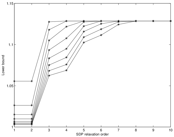
Figure 1: Lower bounds for SDP relaxations of problem (10) on bounded sets $K=[-R,\>R]$ for $R=2$ (top curve) to $R=9$ (bottom curve).

On Figure 1 we report the sequences of lower bounds obtained by solving the SDP relaxations of problem (10) on compact sets $\mathbf{K}=[-R,\>R]$ for $R=2,3,\ldots,9$.

4.3 Exploiting sparsity with GloptiPoly

Even though version 3 of GloptiPoly is designed to exploit problem sparsity, there is no illustration of this feature in the software user’s guide [5]. In this section we provide such a simple example. Note also that GloptiPoly is not able to detect sparsity in a given problem, contrary to SparsePOP which uses a heuristic to find chordal extensions of graphs [12]. However, SparsePOP is not designed to handle directly rational optimization problems.

Consider the elementary example of [7, Section 3.2]:

$$\begin{array}[]{ll}\inf_{\mathbf{x}\in\mathbb{R}^{4}}&x_{1}x_{2}+x_{1}x_{3}+x_{1}x_{4}\\ \mathrm{s.t.}&x^{2}_{1}+x^{2}_{2}\leq 1\\ &x^{2}_{1}+x^{2}_{3}\leq 2\\ &x^{2}_{1}+x^{2}_{4}\leq 3\end{array}$$

for which the variable index subsets $I_{1}=\{1,2\}$, $I_{2}=\{1,3\}$, $I_{3}=\{1,4\}$ satisfy the running intersection property of Definition 3.1. Note that this problem is a particular case of (1) with a polynomial objective function.

Without exploiting sparsity, the GloptiPoly script to solve this problem is as follows:

mpol x1 x2 x3 x4
Pdense = msdp(min(x1*x2+x1*x3+x1*x4), ...
         x1^2+x2^2<=1,x1^2+x3^2<=2,x1^2+x4^2<=3,2);
[stat,obj] = msol(Pdense);

GloptiPoly certifies global optimality with a moment matrix of size 15, and 3 localizing matrices of size 5. And here is the script exploiting sparsity, splitting the variables into several measures $\mu_{i}$ consistently with subsets $I_{i}$:

mpol x1 3
mpol x2 x3 x4
mu(1) = meas([x1(1) x2]); % first measure on x1 and x2
mu(2) = meas([x1(2) x3]); % second measure on x1 and x3
mu(3) = meas([x1(3) x4]); % third measure on x1 and x4
f = mom(x1(1)*x2)+mom(x1(2)*x3)+mom(x1(3)*x4); % objective function
k = 3; % SDP relaxation order
m1 = mom(mmon(x1(1),k)); % moments of first measure
m2 = mom(mmon(x1(2),k)); % moments of second measure
m3 = mom(mmon(x1(3),k)); % moments of third measure
K = [x1(1)^2+x2^2<=1, x1(2)^2+x3^2<=2, x1(3)^2+x4^2<=3]; % supports
Psparse = msdp(min(f),m1==m2,m3==m2,K,mass(mu)==1);
[stat,obj] = msol(Psparse);

GloptiPoly certifies global optimality with 3 moment matrices of size 6, and 3 localizing matrices of size 3.

4.4 Comparison with the epigraph approach

In most of the examples we have processed, the epigraph approach described in the Introduction (consisting of introducing one lifting variable for each rational term in the objective function) was less efficient than the GMP approach. Typically, the order of the SDP relaxation (and hence its size) required to certify global optimality is typically larger with the epigraph approach.

When evaluating the epigraph approach, we also observed that it is numerically preferable to replace the inequality constraints $r_{i}q_{i}(\mathbf{x})-p_{i}(\mathbf{x})\geq 0$ with equality constraints $r_{i}q_{i}(\mathbf{x})-p_{i}(\mathbf{x})=0$ in the definition of semi-algebraic set $\hat{\mathbf{K}}$ in (3). For the example of Section 4.1 the epigraph approach with inequalities certifies global optimality at order $k=5$, whereas the epigraph approach with equalities requires $k=1$.

As a typical illustration of the issues faced with the epigraph approach consider the example with eighth-degree terms

$$\inf_{\mathbf{x}\in\mathbb{R}^{2}}f(x)=\sum_{i=1}^{10}\frac{(x_{1}+x_{2})(x^{2}_{1}+x^{2}_{1}x^{2}_{2}+x^{4}_{2}+i^{2})-(ix^{2}_{2}+1)(x^{4}_{1}+x^{2}_{2}+2i)}{(x^{4}_{1}+x^{2}_{2}+2i)(x^{2}_{1}+x^{2}_{1}x^{2}_{2}+x^{4}_{2}+i^{2})}$$ (11)

which is cooked up to have several local optima and sufficiently high degree to prevent reduction to the same denominator. After a suitable scaling to make critical points fit within the box $[-1,1]^{2}$, as required by the moment SDP relaxations formulated in the power basis [4, Section 6.5], the GMP approach yields a certificate of global optimality with $x^{*}_{1}=-0.60450$, $x^{*}_{2}=-2.2045$, $f^{*}=-6.2844$ at order $k=6$ in a few seconds on a standard PC. In contrast, the epigraph approach does not provide a certificate for an order as high as $k=10$, requiring more than one minute of CPU time.

4.5 Shekel’s foxholes

Consider the modified Shekel foxholes rational function minimization problem [2]

$$\min_{x\in{\mathbb{R}}^{n}}\sum_{i=1}^{N}\frac{1}{\sum_{j=1}^{n}(x_{j}-a_{ij})^{2}+c_{i}}$$ (12)

whose data $a_{ij}$, $c_{i}$, $i=1,\ldots,N$, $j=1,\ldots,n$ can be found in [1, Table 16]. This function is designed to have many local minima, and we know the global minimum in the case $n=5$, see [1, Table 17]. After a suitable scaling to make critical points fit within the box $[0,1]^{5}$, and after addition of a Euclidean ball constraint centered in the box, the GMP approach yields a certificate of global optimality at order $k=3$ in less than one minute on a standard PC. The extracted minimizer is $x^{*}_{1}=8.0254$, $x^{*}_{2}=9.1483$, $x^{*}_{3}=5.1138$, $x^{*}_{4}=7.6213$, $x^{*}_{5}=4.5638$, which matches with the known global minimizer to four significant digits. This point can be refined if given an initial guess for a local optimization method. If we use a standard quasi-Newton BFGS algorithm, we obtain after a few iterations a point matching the known global minimizer to eight significant digits.

In the case $n=10$, for which the global minimum is given in [1, Table 17], the GMP approach yields a certificate of global optimality at order $k=2$ in about 750 seconds of CPU time. Here too, we observe that the extracted minimizer $x^{*}_{1}=8.0249$, $x^{*}_{2}=9.1518$, $x^{*}_{3}=5.1140$, $x^{*}_{4}=7.6209$, $x^{*}_{5}=4.5640$, $x^{*}_{6}=4.7110$, $x^{*}_{7}=2.996$, $x^{*}_{8}=6.1259$, $x^{*}_{9}=0.73424$, $x^{*}_{1}0=4.9820$ is a good approximation to the minimizer, with four correct significant digits. If necessary, this point can be used as an initial guess for refining with a local solver.

Note that it is not possible to exploit problem sparsity in this case, since all the variables appear in each term in sum (12).

4.6 Rosenbrock’s function

Consider the rational optimization problem

$$f^{*}=\max_{x\in{\mathbb{R}}^{n}}\sum_{i=1}^{n-1}\frac{1}{100(x_{i+1}-x^{2}_{i})^{2}+(x_{i}-1)^{2}+1}$$ (13)

which has the same critical points as the well-known Rosenbrock problem

$$\min_{x\in{\mathbb{R}}^{n}}\sum_{i=1}^{n-1}(100(x_{i+1}-x^{2}_{i})^{2}+(x_{i}-1)^{2})$$

whose geometry is troublesome for local optimization solvers. It can been easily shown that the global maximum $f^{*}=1$ of problem (13) is achieved at $x^{*}_{i}=1$, $i=1,\ldots,n$. Our experiments with local optimization algorithms reveal that standard quasi-Newton solvers or functions of the Optimization toolbox for Matlab, called repeatedly with random initial guesses, typically yield local maxima quite far from the global maximum.

With our GMP approach, after exploiting sparsity and adding bound constraints $x^{2}_{i}\leq 16$, $i=1,\ldots,n$, we could solve problem (13) with a certificate of global optimality for $n$ up to $1000$. Typical CPU times range from 10 seconds for $n=100$ to 500 seconds for $n=1000$.

5 Conclusion

The problem of minimizing the sum of many low-degree (typically non-convex) rational fractions on a (typically non-convex) semi-algebraic set arises in several important applications, and notably in computer vision (triangulation, estimation of the fundamental matrix in epipolar geometry) and in systems control ($H_{2}$ optimal control with a fixed-order controller of a linear system subject to parametric uncertainty). These engineering problems motivated our work, but the application of our techniques to computer vision and systems control will be described elsewhere. These fractional programming problems being non convex, local optimization approaches yield only upper bounds on the optimum.

In this paper we were interested in computing the global minimum (and possibly global minimizers) or at least, computing valid lower bounds on the global minimum, for fractional programs involving a sum with many terms. We have used a semidefinite programming (SDP) relaxation approach by formulating the rational optimization problem as an instance of the generalized moment problem (GMP). In addition, problem structure can be sometimes exploited in the case where the number of variables is large but sparsity is present. Numerical experiments with our public-domain software GloptiPoly interfaced with off-the-shelf semidefinite programming solvers indicate that the approach can solve problems that can be challenging for state-of-the-art global optimization algorithms. This is consistent with the experiments made in [3] where the (dense) SDP relaxation approach was first applied to (polynomial) optimization problems of computer vision.

For larger and/or ill-conditioned problems, it can happen that GloptiPoly extracts from the moment matrix a minimizer which is not very accurate. It can also happen that GloptiPoly is not able to extract a minimizer, in which case first-order moments approximate the minimizer (provided it is unique, which is generically true for rational optimization). The approximate minimizer can be then input to any local optimization algorithm as an initial guess.

A comparison of our approach with other techniques of global optimization (reported e.g. on Hans Mittelmann’s or Arnold Neumaier’s webpages) is out of the scope of this paper. We believe however that such a comparison would be fair only if no expert tuning is required for alternative algorithms. Indeed, when using GloptiPoly the only assumption we make is that we know a ball containing the global optimizer. Besides this, our results are fully reproducible (Matlab files reproducing our examples are available upon request) and our SDP relaxations are solved with general-purpose semidefinite programming solvers.

References

• [1] M. M. Ali, C. Khompatraporn, Z. B. Zabinsky. A numerical evaluation of several stochastic algorithms on selected continuous global optimization test problems. J. Global Optim., 31(4):635-672, 2005.
• [2] H. Bersini, M. Dorigo, S. Langerman, G. Seront, L. Gambardella. Results of the first international contest on evolutionary optimisation. IEEE Intl. Conf. Evolutionary Computation, Nagoya, Japan, 1996.
• [3] F. Kahl, D. Henrion. Globally optimal estimates for geometric reconstruction problems. IEEE Intl. Conf. Computer Vision, Beijing, China, 2005.
• [4] D. Henrion, J. B. Lasserre. GloptiPoly: global optimization over polynomials with Matlab and SeDuMi. ACM Trans. Math. Software, 29:165–194, 2003.
• [5] D. Henrion, J. B. Lasserre, J. Löfberg. GloptiPoly 3: moments, optimization and semidefinite programming. Optim. Methods and Software, 24:761–779, 2009.
• [6] D. Jibetean, E. de Klerk. Global optimization of rational functions: a semidefinite programming approach. Math. Programming, 106:93-109, 2006.
• [7] J. B. Lasserre. Convergent SDP relaxations in polynomial optimization with sparsity. SIAM J. Optim., 17:822-843, 2006.
• [8] J. B. Lasserre. A semidefinite programming approach to the generalized problem of moments. Math. Programming, 112:65-92, 2008.
• [9] J. B. Lasserre. Moments, positive polynomials and their applications, Imperial College Press, London, 2009.
• [10] S. Schaible, J. Shi. Fractional programming: the sum-of-ratios case. Optim. Methods Software, 18(2):219–229, 2003.
• [11] S. Waki, S. Kim, M. Kojima, M. Muramatsu. Sums of squares and semidefinite programming relaxations for polynomial optimization problems with structured sparsity. SIAM J. Optim., 17:218-242, 2006.
• [12] H. Waki, S. Kim, M. Kojima, M. Muramatsu, H. Sugimoto. SparsePOP: a sparse semidefinite programming relaxation of polynomial optimization problems. ACM Trans. Math. Software, 35:1-13, 2008.