(2+1)D surface solitons at the interface between a linear medium and a nonlocal nonlinear medium

Abstract

We address (2+1)D surface solitons occurring at the interface between a linear medium and a nonlocal nonlinear medium whose nonlinear contribution to the refractive index has a initial value at the interface. We find that there exist stable single and dipole surface solitons which do not exhibit a power threshold. The properties of the surface solitons can be affected by the initial value and the degree of nonlocality. When a laser beam is launched away from the interface, the beam will be periodic oscillations.

I Introduction

Nonlocal spatial solitons have been investigated for decades both theoretically and experimentally. Spatially nonlocality is a generic property in different materials including the photorefractive media ref1 ; ref2 , thermal nonlinear media ref3 ; ref4 ; ref5 ; ref6 ; ref7 , liquid crystals ref8 ; ref9 ; ref10 ; ref11 ; ref12 ; ref12-1 , and so on. Nonlocality can lead to new kinds of waves that would have been otherwise impossible in local nonlinear media. Especially, for two-dimensional media with different types of nonlocal response, they can support stationary multipoles ref13 ; ref14 ; ref15 ; ref16 ; ref17 ; ref18 , stable vortices ref19 ; ref20 ; ref21 ; ref22 ; ref23 , and rotating ref24 ; ref25 and spiraling ref5 ; ref26 soliton states.

Surface waves localized at the interface of two different optical materials have many novel properties, which have been studied in nonlocal media recently. The light beam trajectory can be strongly affected by the presence of interfaces, because beams propagating in nonlocal media cause refractive index changes in regions far exceeding the beam width. Under proper conditions, stationary surface waves can propagate along the interface in both local nonlinear media ref27 ; ref28 ; ref29 ; ref30 and nonlocal nonlinear media ref31 ; ref32 ; ref33 ; ref34 ; ref35 ; ref36 ; ref37 ; ref38 .

Thermal media ref33 ; ref34 ; ref37 and photorefractive crystals ref38 have been also utilized to demonstrate (2+1)D surface solitons. In this paper, we will study (2+1)D surface solitons occurring at the interface between a linear medium and a nonlocal nonlinear medium whose nonlinear contribution to the refractive index has a initial value at the interface. We find that there exist single surface solitons at the edge and the corner of the two 2D media and dipole surface solitons at the edge of the two 2D media. These stable solitons do not exhibit a power threshold. The positions of the peak values and full width at half maximum(FWHM) of the surface solitons can be affected by the degree of nonlocality. However, the initial value can only influence the positions of the peak values of the surface solitons. In addition, when a laser beam is launched away from the interface, the beam will be periodic oscillations, even if the launch position is far away from the interface.

II Theoretical Model

Considering a laser beam propagating along the interface between a nonlocal nonlinear medium and a linear medium, the complex amplitude $E(X,Y,Z)$ of the light field satisfies the scalar wave equation ref31 ; ref33 ; ref38

$$\nabla_{XY}^{2}E+\frac{\partial^{2}E}{\partial Z^{2}}+k_{0}^{2}n^{2}E=0,$$ (1)

where $k_{0}=2\pi/\lambda$ is the wave number in vacuum, and $n=n_{L}+\Delta n$ for the nonlinear medium($X\leq 0$) and $n=n_{0}$ for the linear medium($X\geq 0$). $\Delta n$ represents the nonlinear contribution to the refractive index and may originate from any diffusive nonlinear effect, which can be written by ref31

$$w_{m}^{2}\nabla_{XY}^{2}\Delta n-\Delta n+n_{2}|E|^{2}=0,$$ (2)

where $w_{m}$ is the characteristic length of the nonlinear response and $n_{2}$ is the nonlinear index coefficient. For the local case, $w_{m}\rightarrow 0$, we have $\Delta n=n_{2}|E|^{2}$.

Let us put $E(X,Y,Z)=E_{0}(X,Y,Z)\exp(i\beta Z)$ and submit into the equation (1) and (2). Then, using the slowly varying envelope approximation and introducing the normalized variables $x=X/w_{0},y=Y/w_{0},z=Z/(\beta w_{0}^{2}),a=k_{0}w_{0}\sqrt{n_{2}n_{L}}E_{0}$ and $\phi=k_{0}^{2}w_{0}^{2}n_{L}\Delta n$, we get

$$\frac{1}{2}\nabla_{\bot}^{2}a+i\partial_{z}a+\beta_{1}a+\phi a=0\quad\textrm{for}\quad x\leq 0,$$ (3a)

$$\frac{1}{2}\nabla_{\bot}^{2}a+i\partial_{z}a+\beta_{2}a=0\quad\textrm{for}\quad x\geq 0,$$ (3b)

and

$$d^{2}\nabla_{\bot}^{2}\phi-\phi+|a|^{2}=0\quad\textrm{for}\quad x\leq 0,$$ (4)

where $\nabla_{\bot}^{2}=\partial_{x}^{2}+\partial_{y}^{2}$, $\beta_{1}=w_{0}^{2}(k_{0}^{2}n_{L}^{2}-\beta^{2})/2$, $\beta_{2}=w_{0}^{2}(k_{0}^{2}n_{0}^{2}-\beta^{2})/2$, $\beta$ is the wave number in the media, $w_{0}$ is the beam width, and $d=w_{m}/w_{0}$ stands for the degree of nonlocality of the nonlinear response. For $x\leq 0$, the equations describe a local nonlinear response as $d\rightarrow 0$ and a strongly nonlocal response as $d\rightarrow\infty$.

We search for stationary soliton solutions of Eqs. (3) and (4) numerically in the form $a(x,y,z)=u(x,y)\exp(ibz)$, where $u$ is the real function and $b$ is a real propagation constant of spatial solitons in the normalized system.

$$\frac{1}{2}\nabla_{\bot}^{2}u-bu+\beta_{1}u+\phi u=0\quad\textrm{for}\quad x\leq 0,$$ (5a)

$$\frac{1}{2}\nabla_{\bot}^{2}u-bu+\beta_{2}u=0\quad\textrm{for}\quad x\geq 0,$$ (5b)

and

$$d^{2}\nabla_{\bot}^{2}\phi-\phi+|u|^{2}=0\quad\textrm{for}\quad x\leq 0.$$ (6)

III Numerical results

III.1 Single surface solitons

We firstly talk about new surface-wave soliton solutions at the edge of the two 2D media. Here, we assume that the normalized nonlinear contribution to the refractive index at the interface($y=0$) has a initial value $\phi_{d}(\phi_{d}>0)$. The boundary conditions for the fields at the interface are the continuity of the transverse field($a(y\rightarrow 0_{-})=a(y\rightarrow 0_{+})$) and its derivative($da(y\rightarrow 0_{-})/dy=da(y\rightarrow 0_{+})/dy$). Because the width of the surface solitons is much smaller than the sample width, $a$ and $\phi$ vanishes at the other boundary.

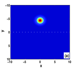
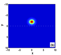
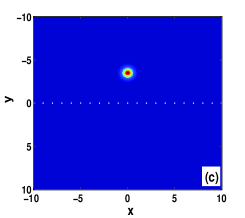
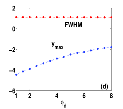
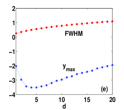
Figure 1: Sketch of 2D single surface solitons at the edge of the interface with (a) $\phi_{d}=1$, $d=20$, (b) $\phi_{d}=7$, $d=20$ and (c) $\phi_{d}=7$, $d=5$. The positions of the peak values $y_{max}$ and FWHM versus (d) the boundary value $\phi_{d}$ and (e) the nonlocal degree $d$. White dashed line indicates interface position. All quantities are plotted in arbitrary dimensionless units.

Three different solitons are separately shown in Fig. 1(a), (b) and (c). We can easily see that the soliton is closely attached to the interface with $\phi_{d}=7$ and $d=20$ in Fig. 1(b), but the solitons are farther detached from the interface with $\phi_{d}=1$ and $d=20$ in Fig. 1(a) or $\phi_{d}=7$ and $d=5$ in Fig. 1(c). Obviously, $\phi_{d}$ and $d$ influence the position or shape of the solitons. To further explain this point, we see that the positions of the peak values($y_{max}$) and FWHM of the surface wave solitons versus the boundary value $\phi_{d}$(Fig. 1(d)) at the interface or the degree of nonlocality $d$(Fig. 1(e)). From Fig. 1(d), we can see that, under the condition($d=20$), the soliton will be attracted to the interface and more and more significant part of their optical power residing in the linear meidium as $\phi_{d}$ increases. That is to say, $\phi_{d}$ is larger, the larger a “surface force” exerted on the beam by the interface. However, $\phi_{d}$ cannot influence the beam width of solitons. From Fig. 1(e), at $\phi_{d}=7$, the changing of the refractive index of the nonlocal nonlinear medium induced by $d$ results in the changing of FWHM and $y_{max}$ of the solitons. Because of the changing of FWHM, $y_{max}$ changes intricately, though a force exerted on the beam by the degree of nonlocality increases all the while.

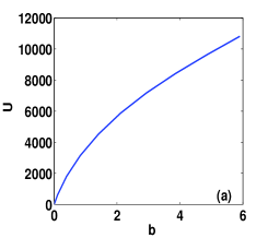
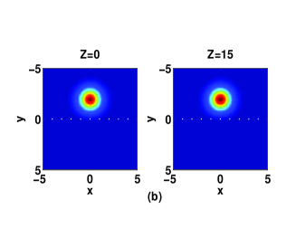
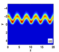
Figure 2: (a) Energy flow $U$ versus the propagation constant $b$ with $d=20$ and $\phi_{d}=7$. (b) Stable propagation of surface solitons in Fig.1(b)with noise $\sigma^{2}_{noise}=0.05$ for a distance of 15 diffraction lengths. (c) Trajectories of the incident beam with the beam center coordinates $y=-1.99\mu m$. White dashed line indicates interface position. All quantities are plotted in arbitrary dimensionless units.

Fig. 2(a) shows that the energy flow $U=\int_{-\infty}^{\infty}\int_{-\infty}^{\infty}|a|^{2}dxdy$ of the single 2D surface solitons monotonically increases with $b$ where $dU/db>0$. This shows that the solitons are stable ref32 ; ref33 . Here, to further elucidate the stability of the surface solitons, we do the direct numerical simulations of Eqs. (3) and (4) with input conditions $a|_{Z=0}=u(1+\rho)$, where $\rho(x,y)$ is a broadband random perturbation. The fact which is shown in Fig. 2(b) confirms the result of Fig. 2(a). Then we proceed to address the dynamics behavior of the propagation of surface solitons. For convenience, the (1+1)D circumstance is considered. Fig. 2(c) depicts that a narrow beam is launched $y=-1.99\mu m$ away from the interface. The beam maintains a localized shape. However, it is oscillation in a fully periodic fashion in the virtue of the cooperation of the forces exerted by the boundary and the nonlocal nonlinearity, even if the launch position is far away from the opsition of the surface soliton ref33 .

Next, we consider that new soliton solutions at the corner of the two 2D media. Here, we assume that the normalized nonlinear contribution to the refractive index at $x=0$ and $y=0$ have a initial value $\phi=\phi_{d}(\phi_{d}>0)$. The boundary conditions for the fields at the interface meet the continuity conditions.

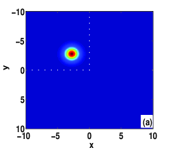
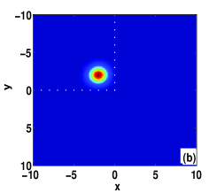
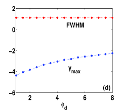
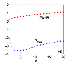
Figure 3: Sketch of 2D single surface solitons at the corner of the interface with (a) $\phi_{d}=5$, $d=20$, (b) $\phi_{d}=10$, $d=20$ and (c) $\phi_{d}=10$, $d=10$. The positions of the peak values $y_{max}$ and FWHM versus (d) the boundary value $\phi_{d}$ and (e) the nonlocal degree $d$. White dashed line indicates interface position. All quantities are plotted in arbitrary dimensionless units.

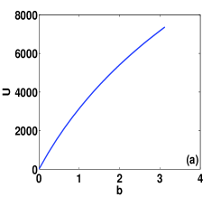
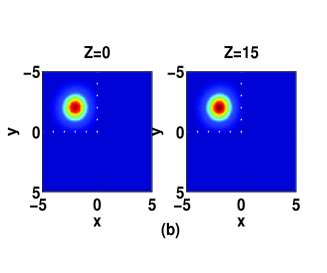
Figure 4: (a) Energy flow $U$ versus the propagation constant $b$ with $d=20$ and $\phi_{d}=10$. (b) Stable propagation of surface solitons in Fig.3(b) with noise $\sigma^{2}_{noise}=0.05$ for a distance of 15 diffraction lengths. White dashed line indicates interface position. All quantities are plotted in arbitrary dimensionless units.

Fig. 3(a), (b) and (c) separately show three different solitons. The soliton is closely attached to the interface with $\phi_{d}=10$ and $d=20$(see Fig. 3(b)), but the solitons are farther detached from the interface with $\phi_{d}=5$ and $d=20$(Fig. 3(a)) or $\phi_{d}=10$ and $d=10$(Fig. 3(c)). To further illustrate the influence of $\phi_{d}$ and $d$ on the solitons, we display that $y_{max}$ and FWHM versus $\phi_{d}$ in Fig. 3(d) or $d$ in Fig. 3(e). The energy flow $U$ monotonically increasing with $b$ shown in Fig. 4(a) and the direct numerical simulations of Eqs. (3) and (4) with noise $\sigma^{2}_{noise}=0.05$ shown in Fig. 4(b) explain that the solitons are stable. The results can be similarly illustrated as the solitons at the edge of the interface.

III.2 Two dimensions dipole surface solitons

In addition to single surface solitons, we also find a 2D stationary dipole surface solitons. The surface solitons are found numerically by a standard relaxation method which converges to a stationary solution after some iterations provided that a suitable guess for initial field distribution. The boundary conditions are the same as the single surface solitons at the edge of the interface.

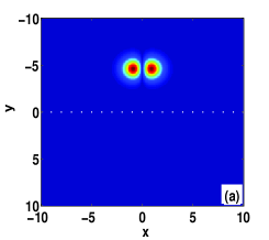
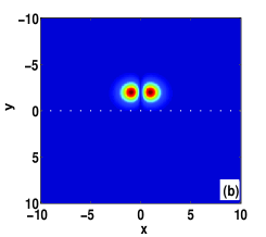
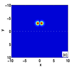
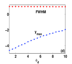
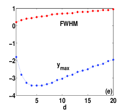
Figure 5: Sketch of 2D dipole surface solitons with (a) $\phi_{d}=1$, $d=20$, (b) $\phi_{d}=10$, $d=20$ and (c) $\phi_{d}=10$, $d=10$. The positions of the peak values $y_{max}$ and FWHM versus (d) the boundary value $\phi_{d}$ and (e) the nonlocal degree $d$. White dashed line indicates interface position. All quantities are plotted in arbitrary dimensionless units.

Fig. 5(b) depicts that the amplitude for a dipole soliton which is closely attached to the interface with $\phi_{d}=10$ and $d=20$. However, the solitons are farther detached from the interface with $\phi_{d}=1$ and $d=20$ in Fig. 5(a) or $\phi_{d}=10$ and $d=10$ in Fig. 5(c). Because the poles of solitons are almost symmetric in the $x$ direction, the changing of $y_{max}$ and FWHM of one pole of the solitons can explain the changing of the position and shape of the dipoles. Fig. 5(d) and (e) shows $y_{max}$ and FWHM as functions of the boundary value $\phi_{d}$ and the degree of nonlocality $d$, respectively.

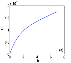
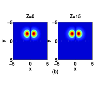
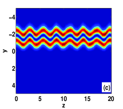
Figure 6: (a) Energy flow $U$ versus the propagation constant $b$ with $d=20$ and $\phi_{d}=10$. (b) Stable propagation of surface solitons in Fig.5(b)with noise $\sigma^{2}_{noise}=0.05$ for a distance of 15 diffraction lengths. (c) Trajectories of the incident beam with the beam center coordinates $y=-1.91\mu m$. White dashed line indicates interface position. All quantities are plotted in arbitrary dimensionless units.

Fig. 6(a) shows that the energy flow monotonically increases with the propagation constant for dipole surface solitons. With increasing energy flow, surface dipoles become more localized, i.e., the distance between poles along the $x$ axis and their widths decrease. To further elucidate the stability of the surface dipoles, we do the direct numerical simulations of Eqs. (3) and (4) with noise $\sigma^{2}_{noise}=0.05$. Particularly, the complex surface solitons are stable in the entire existence domain. Fig. 6(b) depicts a typical evolution dynamic. The considerable input perturbations cannot almost cause oscillations of amplitudes of the two poles forming the dipole, but the dipoles remain their internal structures over huge distances. Contrarily, in a bulk diffusive medium, it is known that weak input perturbations can cause slow but progressively increasing oscillations of the bright spots forming a dipole, resulting specially in their slow decay into fundamental solitons ref34 . So, we think that the presence of a interface possessing a initial value for $\phi$ leads to stabilization of dipole solitons. This is further illustrated by the results of Fig. 6(c). when the beam is launched $y=-1.91\mu m$ away from the interface, the stationary soliton cannot be formed, but it is periodically oscillating. This are very good description of the boundaries of the role of solitons.

IV Conclusion

In conclusion, we have addressed (2+1)D surface solitons occurring at the interface between a linear medium and a nonlocal nonlinear medium whose nonlinear contribution to the refractive index has a initial value at the interface. We find that there exist stable single and dipole surface solitons which do not exhibit a power threshold. The degree of nonlocality have influence on the positions of the peak value and FWHM of the surface solitons, but the initial value can only influence the positions of the peak values of the surface solitons. In addition, when a laser beam is launched away from the interface, the beam will be periodic oscillations, even if the launch position is far away from the interface.

List of Figure Captions

Fig. 1. Sketch of 2D single surface solitons at the edge of the interface with (a) $\phi_{d}=1$, $d=20$, (b) $\phi_{d}=7$, $d=20$ and (c) $\phi_{d}=7$, $d=5$. The positions of the peak values $y_{max}$ and FWHM versus (d) the boundary value $\phi_{d}$ and (e) the nonlocal degree $d$. White dashed line indicates interface position. All quantities are plotted in arbitrary dimensionless units.

Fig. 2. (a) Energy flow $U$ versus the propagation constant $b$ with $d=20$ and $\phi_{d}=7$. (b) Stable propagation of surface solitons in Fig.1(b)with noise $\sigma^{2}_{noise}=0.05$ for a distance of 15 diffraction lengths. (c) Trajectories of the incident beam with the beam center coordinates $y=-1.99\mu m$. White dashed line indicates interface position. All quantities are plotted in arbitrary dimensionless units.

Fig. 3. Sketch of 2D single surface solitons at the corner of the interface with (a) $\phi_{d}=5$, $d=20$, (b) $\phi_{d}=10$, $d=20$ and (c) $\phi_{d}=10$, $d=10$. The positions of the peak values $y_{max}$ and FWHM versus (d) the boundary value $\phi_{d}$ and (e) the nonlocal degree $d$. White dashed line indicates interface position. All quantities are plotted in arbitrary dimensionless units.

Fig. 4. (a) Energy flow $U$ versus the propagation constant $b$ with $d=20$ and $\phi_{d}=10$. (b) Stable propagation of surface solitons in Fig.3(b) with noise $\sigma^{2}_{noise}=0.05$ for a distance of 15 diffraction lengths. White dashed line indicates interface position. All quantities are plotted in arbitrary dimensionless units.

Fig. 5. Sketch of 2D dipole surface solitons with (a) $\phi_{d}=1$, $d=20$, (b) $\phi_{d}=10$, $d=20$ and (c) $\phi_{d}=10$, $d=10$. The positions of the peak values $y_{max}$ and FWHM versus (d) the boundary value $\phi_{d}$ and (e) the nonlocal degree $d$. White dashed line indicates interface position. All quantities are plotted in arbitrary dimensionless units.

Fig. 6. (a) Energy flow $U$ versus the propagation constant $b$ with $d=20$ and $\phi_{d}=10$. (b) Stable propagation of surface solitons in Fig.5(b)with noise $\sigma^{2}_{noise}=0.05$ for a distance of 15 diffraction lengths. (c) Trajectories of the incident beam with the beam center coordinates $y=-1.91\mu m$. White dashed line indicates interface position. All quantities are plotted in arbitrary dimensionless units.

References

- (1) M. Segev, B. Crosignani, A. Yariv, and B. Fischer, “Spatial solitons in photorefractive media,” Phys. Rev. Lett. 68, 923-926 (1992).
- (2) W. Krolikowsky, B. Luther-Davies, and C. Denz, “Photorefractive solitons,” Quantum Electron. 39, 3-12(2003).
- (3) C. Rotschild, O. Cohen, O. Manela, M. Segev, and T. Carmon, “Solitons in nonlinear media with an infinite range of nonlocality: first observation of coherent elliptic solitons and of vortex-ring solitons,” Phys. Rev. Lett. 95, 213904 (2005).
- (4) A. Dreischuh, D. N. Neshev, D. E. Petersen, O. Bang, and W. Krolikowski, “Observation of attraction between dark solitons,” Phys. Rev. Lett. 96, 043901 (2006).
- (5) C. Rotschild, B. Alfassi, O. Cohen, and M. Segev, “Long-range interactions between optical solitons,” Nat. Phys. 2, 769 (2006).
- (6) F. Ye, Bambi. Hu, Y. V. Kartashov, and L. Torner, “Nonlinearity-mediated soliton ejection from trapping potentials in nonlocal media ,” Phys. Rev. A 82, 023822 (2010).
- (7) D. Buccoliero, A. S. Desyatnikov, W. Krolikowski, and Y. S. Kivshar, “Spiraling multivortex solitons in nonlocal nonlinear media,” Opt. Lett. 33, 198-201 (2008).
- (8) C. Conti, M. Peccianti, and G. Assanto, “Observation of optical spatial solitons in a highly nonlocal medium,” Phys. Rev. Lett. 92, 113902 (2004).
- (9) M. Peccianti, K. Brzadkiewicz, and G. Assanto, “Nonlocal spatial soliton interactions in nematic liquid crystals,” Opt. Lett. 27, 1460-1462 (2002).
- (10) M. Peccianti, C. Conti, G. Assanto, A. De Luca, and C. Umeton, “Routing of anisotropic spatial solitons and modulational instability in nematic liquid crystals,” Nature 432, 733 C737 (2004).
- (11) A. Alberucci, M. Peccianti, G. Assanto, A. Dyadyusha, and M. Kaczmarek, “Two-color vector solitons in nonlocal media,” Phys. Rev. Lett. 97, 153903 (2006).
- (12) A. A. Minzoni, N. F. Smyth, and Z. Xu, “Stability of an optical vortex in a circular nematic cell,” Phys. Rev. A 81, 033816 (2010)
- (13) A. Alberucci, A. Piccardi, M. Peccianti, M. Kaczmarek, and G. Assanto, “Propagation of spatial optical solitons in a dielectric with adjustable nonlinearity,” Phys. Rev. A 82, 023806 (2010)
- (14) C. Rotschild, M. Segev, Z. Xu, Y. V. Kartashov, L. Torner, and O. Cohen, “Two-dimensional multipole solitons in nonlocal nonlinear media,” Opt. Lett. 31, 3312-3314(2006).
- (15) S. Skupin, O. Bang, D. Edmundson, and W. Krolikowski,“Stability of two-dimensional spatial solitons in nonlocal nonlinear media ,” Phys. Rev. E 73, 066603(2006).
- (16) A. I. Yakimenko, V. M. Lashkin, and O. O. Prikhodko, “Dynamics of two-dimensional coherent structures in nonlocal nonlinear media,” Phys. Rev. E 73, 066605(2006).
- (17) Y. V. Kartashov, L. Torner, V. A. Vysloukh, and D. Mihalache, “Multipole vector solitons in nonlocal nonlinear media ,” Opt. Lett. 31, 1483-1485(2006).
- (18) D. Buccoliero, A. S. Desyatnikov,W. Krolikowski, and Y. S. Kivshar, “Laguerre and Hermite soliton clusters in nonlocal nonlinear media,” Phys. Rev. Lett. 98, 053901(2007).
- (19) V. M. Lashkin, “Two-dimensional nonlocal vortices, multipole solitons, and rotating multisolitons in dipolar Bose-Einstein condensates,” Phys. Rev. A 75, 043607(2007).
- (20) V. I. Kruglov, Y. A. Logvin, and V. M. Volkov, “The theory of spiral laser beams in nonlinear media,” J. Mod. Opt. 39, 2277-2291(1992).
- (21) D. Briedis, D. Petersen, D. Edmundson, W. Krolikowski, and O. Bang, “Ring vortex solitons in nonlocal nonlinear media,” Opt. Express 13, 435-443(2005).
- (22) A. I. Yakimenko, Y. A. Zaliznyak, and Y. Kivshar, “Stable vortex solitons in nonlocal self-focusing nonlinear media,” Phys. Rev.E 71, 065603(R)(2005).
- (23) C. Rotschild, O. Cohen, O. Manela, M. Segev, and T. Carmon, “Two-dimensional multipole solitons in nonlocal nonlinear media,” Phys. Rev. Lett. 95, 213904(2005).
- (24) Y. V. Kartashov, V. A. Vysloukh, and L. Torner, “Stability of vortex solitons in thermal nonlinear media with cylindrical symmetry,” Opt. Express 23, 9378-9384(2007).
- (25) S. Lopez-Aguayo, A. S. Desyatnikov, Y. S. Kivshar, S. Skupin, W. Krolikowski, and O. Bang, “Stable rotating dipole solitons in nonlocal optical media,” Opt. Lett. 31, 1100-1102(2006).
- (26) S. Lopez-Aguayo, A. S. Desyatnikov, and Y. S. Kivshar, “Azimuthons in nonlocal nonlinear media,” Opt. Express 14, 7903-7908(2006).
- (27) A. Fratalocchi, A. Piccardi, M. Peccianti, and G. Assanto, “Nonlinearly controlled angular momentum of soliton clusters,” Opt. Lett. 32, 1447-1449(2007).
- (28) W. J. Tomlinson, “Surface wave at a nonlinear interface,” Opt. Lett. 5, 323-325 (1980).
- (29) N. N. Akhmediev, V. I. Korneev, and Y. V. Kuz menko, “Excitation of nonlinear surface waves by Gaussian light beams,” Sov. Phys. JETP 61, 62-67 (1985).
- (30) A. D. Boardman. A. A. Maradudin, G. I. Stegeman, T. Twardowski and E. M. Wright, “Exact theory of nonlinear p-polarized optical waves,” Phys. Rev. A. 35, 1159-1164 (1987).
- (31) D. Mihalache, G. Stegeman, C. T. Seaton, R. zanoni, A. D. Boardman and T. Twardowski, “Exact dispersion relations for transverse magnetic polarized guided waves at a nonlinear interface,” Opt. Lett. 12, 187-189 (1987).
- (32) P. Varatharajah, A. Aceves, J. V. Moloney, D. R. Heatley, and E. M. Wright, “Stationary nonlinear surface waves and their stability in diffusive Kerr media,” Opt. Lett. 13, 690-692 (1988).
- (33) Y. V. Kartashov, L. Torner, and V. A. Vysloukh, “Lattice-supported surface solitons in nonlocal nonlinear media,” Opt. Lett. 31, 2595-2597 (2006).
- (34) B. Alfassi, C. Rotschild, O. Manela, M. Segev, and D. N. Christodoulides, “Nonlocal surface-wave solitons,” Phys. Rev. Lett. 98, 213901 (2007).
- (35) F. Ye, Y. V. Kartashov, and L. Torner, “Nonlocal surface dipoles and vortices,” Phys. Rev. A 77, 033829 (2008).
- (36) Y. V. Kartashov, F. Ye, V. A. Vysloukh, and L. Torner, “Surface waves in decofusing thermal media,” Opt. Lett. 32, 2260-2262 (2007).
- (37) Y. V. Kartashov, V. A. Vysloukh, and L. Torner, “Multipole surface solitons in thermal media,” Opt. Lett. 34, 283-285 (2009).
- (38) Y. V. Kartashov, V. A. Vysloukh, and L. Torner, “Ring surface waves in thermal nonlinear media,” Opt. Express 15, 16216-16221 (2007).
- (39) H. Z. Kang, T. H. Zhang, B. H. Wang, C. B. Lou, B. G. Zhu, H. H. Ma, S. M. Liu, J. G. Tian, and J. J. Xu, “(2+1)D surface solitons in virtue of the cooperation of nonlocal and local nonlinearities,” Opt. Lett. 34,3298-3300(2009).