Topological view on magnetic adatoms in graphene

Abstract

We study theoretically the physical properties of a magnetic impurity in graphene. The theory is based on the Anderson model with a very strong Coulomb interaction on the impurity. We start from the Slave-Boson method and introduce a topological picture consisting of a degree of a map and a winding number (WN) to analyze the phase shift and the occupation on the impurity. The occupation is linked to the WN. For a generic normal metal we find a fractional WN. In contrast, the winding is accelerated by the relativistic dispersion of graphene at half-filling in which case an integer occupation is realized. We show that the renormalization that shifts the impurity level is insufficient to invert the sign of the energy level. Consequently, the state at half-filling is stable unless a gate voltage is tuned such that the Fermi level touches the edge of the broadened impurity level. Only in this case the zero field susceptibility is finite and shows a pronounced peak structure when scanning the gate voltage.

I Introduction

Graphene has attracted many theoretical and experimental researches due to its unique properties which are also of relevance for technological applications graphene ; neto . The hallmark of graphene, a monolayer of carbon atoms, is its electronic structure with the valence and the conduction bands touching at two inequivalent points $K_{\pm}$ at the corners of the first Brillouin zone (FBZ). The low energy dispersion around $K_{\pm}$ is relativistic (linear in momentum), with a massless Dirac fermion behavior neto . Of a particular interest is the issue of how the nature of graphene is manifested in the behavior of magnetic adatoms meyer ; cornaglia ; zhuang ; kotov ; uchoa ; ding ; uchoa0906 ; hentschel ; dora ; sengupta ; jacob ; dellanna ; zhu10 ; zhu09 ; zhu10_2 , a topic at the heart of many-body physics, and especially the Kondo effect kotov ; uchoa ; ding ; uchoa0906 ; hentschel ; dora ; sengupta ; jacob ; dellanna ; zhu10 . The Kondo model with a linear dispersion withoff and the Anderson model in $d$-wave superconductors zhang have been investigated already. As detailed below however, for the particular case of magnetic adatoms on graphene some additional features emerge.
The problem of adatoms on graphene was treated within the Hatree-Fock approximation uchoa ; ding ; uchoa0906 . This is only valid at temperatures $T>T_{K}$, where $T_{K}$ is the Kondo temperature. The anisotropic single channel Kondo model hentschel and the Anderson model dora for infinite Coulomb correlation ($U$) were also considered. A Fermi liquid behaviour dora were concluded. In contrast, Ref. sengupta arrives at a two-channel Kondo in graphene due to the valley degeneracy of the Dirac electrons leading to an over-screening and thus to a non-Fermi-liquid-like ground state. In Ref. zhu10 , we conducted a detailed symmetry group analysis to clarify the appropriate physical model and highlighted the various relevant symmetries that are realized depending on whether (A) the adatom is above one carbon atom or (B) this atom is in the center of the honeycomb. The contributions from the two Dirac cones are mixed. For the case B we found generally a multi-channel, multi-flavor Kondo model. While for A we inferred a one-channel, two-flavor behavior. To identify the correct starting Hamiltonian a symmetry analysis is imperative. For example, the detailed symmetry analysis in zhu10 for the A and B cases yields that the realized symmetry groups are $\bar{C}_{3v}$ and $C_{6v}$ point groups. To be consistent with these symmetries, the eigenstates for pure graphene at Dirac points should be recombined as to reflect the modifications imparted by the impurity. As a consequence, a single half spin with zero orbital angular momentum is decoupled from graphene in case B (in contrast Ref. uchoa2011, ).

In this work, we focus on the situation A and consider a two-flavor Anderson model with a relativistic dispersion relation. Therefore, the effect of the gate voltage can be studied in a wide spectrum since the charge fluctuations are already taken into account footnote . We introduce a geometrical picture in form of a winding number (WN) and a degree of a map, to analyze the occupation and the phase shift. It is shown that the occupation takes on the values 0 or 1 when the bare level is respectively above or below the Fermi energy at half-filling. In the presence of a gate voltage, our analytical and the numerical calculations show that the state remains stable only when the edge of the broadened impurity level touches the Fermi energy where a nonzero susceptibility occurs. These findings are traced back mainly to the relativistic dispersion in graphene. In section II, an appropriate formulation is worked out, followed by the topological interpretation in the section III. In section IV, numerical illustrations are displayed for the half-filling case and beyond. In section V, the renormalization of the impurity level and the occupation dependence on the varying gate voltage are calculated. We conclude with a summary of this study.

II Framework

We start from the Anderson Hamiltonian zhu10

$$H=H_{\text{g}}+H_{\text{hyb}}+H_{\text{im}}$$

where the terms $H_{\text{g}}$, $H_{\text{hyb}}$, and $H_{\text{im}}$ describe respectively graphene, the hybridization, and the impurity. The graphene Hamiltonian reads zhu10

$$H_{\text{g}}=\sum_{s\sigma}\int_{-k_{c}}^{k_{c}}dk\varepsilon_{k}c_{sk\sigma}^{\dagger}c_{sk\sigma},$$

where $\varepsilon_{k}=\hbar v_{F}k$, and $v_{F}$ is the Fermi velocity, $s$ and $\sigma$ are valley and spin indices. $k_{c}$ is the cut-off momentum that sets the linear dispersion region. $c_{sk\sigma}$ is an annihilation operator of the one electron state $|sk\sigma\rangle$. The Hamiltonian of the impurity is treated in the $U\rightarrow\infty$ limit, in a standard way hewson ; coleman . We introduce a bosonic field $b$ to guarantee the ($Q$) charge conservation

$$Q=b^{\dagger}b+n_{f}=1,$$

where

$$n_{f}=\sum_{\sigma}f_{\sigma}^{\dagger}f_{\sigma},$$

and $f_{\sigma}$ is the annihilation operator of an electronic state on the impurity with spin $\sigma$. Within the slave-boson (SB) model $H$ reads then

$$H=\tilde{\varepsilon}_{0}n_{f}+H_{\text{g}}+H_{\text{hyb}}+\lambda(b^{\dagger}b-1).$$

Here the normalized impurity energy level is

$$\tilde{\varepsilon}_{0}=\varepsilon_{0}+\lambda.$$

The hybridization Hamiltonian is formulated as

$$H_{\text{hyb}}=v_{0}\sqrt{\pi\Omega_{0}}\sum_{s\sigma}\left(\int\frac{\sqrt{|k|}dk}{2\pi}c_{sk\sigma}^{\dagger}b^{\dagger}f_{\sigma}+h.c.\right).$$ (1)

$v_{0}$ is the hybridization strength, and $\Omega_{0}$ is the area of a unit cell. As usual the bosonic field is assumed to be condensed at the ground state and is described by a renormalization number as

$$\langle b^{\dagger}\rangle=\langle b\rangle=\zeta.$$

$\lambda$ and $\zeta$ are determined by minimizing the free energy which leads to the equations

$$\zeta^{2}=1-\langle n_{f}\rangle$$

and

$$\lambda=-\zeta^{-1}v_{0}\sqrt{\pi\Omega_{0}}\sum_{s\sigma}\int_{-k_{c}}^{k_{c}}dk\frac{\sqrt{|k|}}{2\pi}\langle f_{\sigma}^{\dagger}c_{sk\sigma}\rangle.$$ (2)

The Green’s function associated with the impurity is

$$G_{f\sigma}=z^{-1},\mbox{ where}\quad z=\omega^{+}-\tilde{\varepsilon}_{0}-\zeta^{2}\Sigma_{0}(\omega^{+}),\>\omega^{+}=\omega+i\delta,\;\delta\rightarrow 0^{+}.$$ (3)

The selfenergy is defined as

$$\Sigma_{0}(\omega^{+})=(v_{0}^{2}\Omega_{0}/4\pi)\sum_{s}\int dk|k|(\omega^{+}-\varepsilon_{k})^{-1},$$

and can be given analytically as

$$\Sigma_{0}=-\frac{N_{s}v_{0}^{2}}{2}\left[\rho\ln\frac{|D^{2}-\omega^{2}|}{\omega^{2}}+i\pi|\rho|\theta(D-|\omega|)\right].$$ (4)

The density of state of graphene around the Dirac points reads neto

$$\rho(\omega)=\frac{\Omega_{0}}{2\pi}\frac{\omega}{(\hbar v_{F})^{2}}.$$

Defining the local density of states (LDOS) of the impurity as

$$\mathcal{N}_{f\sigma}=-\frac{\Im}{2\pi}G_{f\sigma},$$

we find

$$\langle n_{f}\rangle=2\int_{-D}^{\varepsilon_{F}}f(\omega)\mathcal{N}_{f\sigma}d\omega,$$ (5)

where $f(\omega)$ is the Fermi function. Following hewson , we derive footnote2

$$\langle n_{f}\rangle=-\frac{1}{\pi}\Im\int_{-D}^{\varepsilon_{F}}d\ln z.$$ (6)

Here we introduced

$$z=r\exp{i[\pi/2-\Theta(\omega,\lambda,\zeta^{2})]},$$

and

$$\Theta(\omega,\lambda,\zeta^{2})=\tan^{-1}\left[\frac{\omega-\tilde{\varepsilon}_{0}-\zeta^{2}\Re\Sigma_{0}}{-\zeta^{2}\Im\Sigma_{0}}\right]$$ (7)

is the phase of $z$ in $(-\pi/2,\pi/2)$. Therefore, the occupation number reads

$$\langle n_{f}\rangle=\frac{1}{2\pi}\int_{-\infty}^{\varepsilon_{F}}d\left(2\Theta(\omega,\lambda,\zeta^{2})\right)=\text{deg(the map)},$$ (8)

which is the Friedel sum rule for an impurity on graphene.

III Topological interpretations

Now we introduce a new picture that allows a topological interpretation by extending the concept of the degree of a map and a WN of a closed curve to an open curve. In Eq. (8), $2\Theta(\omega,\lambda,\zeta^{2})$ defines a map: $O\mapsto P$, where $O$ and $P$ are both 1D manifolds. $O$ stands for the 1D energy region from $-\infty$ to $D$; and the manifold $P$ is ${\cal S}^{1}$. The integral in (8) can be viewed as a winding process by varying the source point $\bar{p}$ (stands for $\varepsilon_{F}$). Simultaneously, the image point $p$ scans in the manifold P shown in Fig. (1a). If $p$ has a cyclic winding, usually an integer for the number of times that the manifold $O$ covers the manifold $P$ is produced and called a WN (similar to the case of a continuous map dubrovin ). Note, our degree of the map $2\Theta$ has the same topological meaning for non-integer WN, it indicates then that the winding process is not complete. We note further, $\Theta$ is the connection in the image manifold $P$, and $\partial\Theta/\partial\omega$ is the curvature of this manifold.

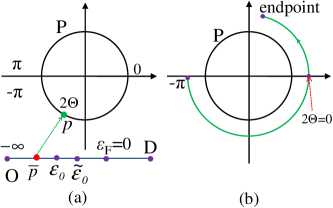
Figure 1: (color online) (a) Schematics of the map from 1D manifold O to P. (b) The winding process for a normal metal.

For a comparison, let us recall the same map for a normal metal with a constant DOS ($\omega\in(-\infty,\varepsilon_{F}]$), i.e.

$$\Theta(\omega)=\tan^{-1}\left((\omega-\varepsilon_{0})/\Delta_{0}\right).$$

When $\bar{p}$ reaches $\varepsilon_{0}$, the image point $p$ attains $\Theta=0$, meaning a half winding of the manifold $P$. When $\bar{p}$ moves over $\varepsilon_{0}$ and approaches the Fermi level $\varepsilon_{F}$, the image point $p$ stops somewhere in the upper branch of the manifold $P$ if $2\Theta\neq\pi$ (see the endpoint in Fig. (1b)). The winding is not completed so that the occupation number is not an integer but a fractional number. In the case that a mean-field SB method is applied and the real part of the selfenergy is ignored, the map reads

$$\Theta(\omega)=\tan^{-1}\left(\frac{\omega-\tilde{\varepsilon}_{0}}{\zeta^{2}\Delta_{0}}\right).$$

If $\zeta$ is not zero, $\varepsilon_{0}$ is renormalized to become $\tilde{\varepsilon}_{0}$ which is mapped onto $\Theta=0$. The $\lambda$ in $\tilde{\varepsilon}_{0}$ gives rise to a shift of the impurity level, and $\zeta^{2}$ changes the winding velocity of the image point.

For the graphene case, we define a function

$$\mathcal{F}(\omega,\lambda,\zeta^{2})=\omega-\zeta^{2}\Re\Sigma_{0}(\omega^{+}),$$ (9)

which is shown in Fig. (2a). The starting point of the winding is fixed at $2\Theta=-\pi$ since $\mathcal{F}\rightarrow-\infty$ as $\omega\rightarrow-\infty$. In Fig. (2a), the solid horizontal line indicates the position of $\tilde{\varepsilon}_{0}$ so that the crossing points with $\mathcal{F}$ indicate the zeros ( $2\Theta=0$ ) of the image points $p$ and the corresponding pre-image points (source points), i.e. $\omega^{*}$s of $\bar{p}$. Counting the number of the pre-image points from the inverse map, generally, there are two points, i.e. $\omega^{*}_{1},\omega_{2}^{*}$, residing closely to $\omega=-D$ in two separated regions, I and II, with opposite countings of the degree of the map. The index of $\omega^{*}_{1}$ ($\omega_{2}^{*}$) is $+1$ ($-1$). The behavior of $\omega=0$ (Dirac point at half-filling) is particularly important for our analysis. As the imaginary part of the selfenergy diminishes, the end of the image point for $\omega=0$ is determined by the relative positions of the function $\mathcal{F}(\omega=0,\lambda,\zeta^{2})$ and $\tilde{\varepsilon}_{0}$. When the former is larger (less) than the latter, the endpoint is $\pi$ ($-\pi$). The linear dispersion around the Dirac points accelerates the phase shift so that the winding process speeds up to the boundary of the manifold $P$.

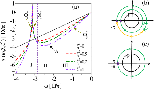
Figure 2: (color online) (a) Numerical graphs for $\mathcal{F}(\omega,\lambda,\zeta^{2})$ and (b) a schematic of the winding process for $\zeta^{2}=1$, $\tilde{\varepsilon}_{0}>0$. In (c) $\zeta^{2}=0$, $\tilde{\varepsilon}_{0}<0$. The energy unit is $D/\pi$. In (a) $\eta=\frac{\Omega_{0}}{2\pi}\frac{v_{0}^{2}}{(\hbar v_{F})^{2}}$ is assumed to be 0.4.

A schematic diagram of such a winding for $\zeta^{2}=1$ and $\tilde{\varepsilon}_{0}>0$ is shown in Fig. (2b). While the first cycle is finished in region (I), in region (II) $p$ comes back from $+\pi$ clockwise to ”A” point, approximately crossing the zero of $2\Theta$ (at $\omega_{2}^{*}$). In region (III), $p$ starts approximately from ”A” winding anticlockwise. However, it does not reach the zero of $2\Theta$ and turns back to $-\pi$ to finish the winding. Hence, a zero winding is concluded for such a case, which is consistent with the condition of minimizing the free energy. Fig. (2c) shows the winding for zero $\zeta^{2}$ and $\tilde{\varepsilon}_{0}<0$ where the WN is 1. We should note that zero $\zeta$ does not mean that there is no effect from graphene to the impurity state. The charge fluctuation still renormalizes the impurity energy level via the parameter $\lambda$ in this case.

It is readily shown that the occupation takes on only the values $0$ or $1$ when $\tilde{\varepsilon}_{0}>0$ or $<0$. For instance, starting initially from $\varepsilon_{0}<0$, $\lambda=0$ and $\zeta^{2}=0$ we obtain the occupation 1. Thus, $\zeta^{2}=0$ is stable against the renormalization process. Starting with $\varepsilon_{0}<0$, $\lambda=0$ and $\zeta^{2}\neq 0$, we find the occupation 1 after one step. This leads to a new $\zeta^{2}=0$. Therefore, we may conclude that the renormalization in graphene is quite different to that in normal metals. When the bare level is below the Fermi level the renormalization effect is small.

IV Numerical illustrations and the case beyond half-filling

Let us consider the effect of a finite gate voltage $v_{\text{g}}$ when the system is away from half-filling. To calculate the susceptibility, we introduce a homogenous, static external magnetic field and let it tend to zero at the end of calculations so that a zero-field susceptibility is obtained. The occupation number and the magnetization of the impurity read

$$\langle n_{f}\rangle=\frac{1}{2\pi}\sum_{\sigma}\int_{-\infty}^{v_{\text{g}}}d\Theta_{\sigma}(\omega,\lambda,\zeta^{2}),$$

and

$$M_{f}=\frac{\mu_{B}}{2\pi}\sum_{\sigma}\int_{-\infty}^{v_{\text{g}}}\sigma d\Theta_{\sigma}(\omega,\lambda,\zeta^{2}),$$

where the phase $\Theta_{\sigma}$ is now spin-dependent containing the spin-dependent $\Sigma_{0\sigma}$, and

$$\tilde{\varepsilon}_{0\sigma}=\tilde{\varepsilon}_{0}-\sigma h,\,h=\frac{1}{2}g\mu_{B}B,$$

where $g$ is the Landé factor, $\mu_{B}$ is the Bohr magneton. To investigate the stability of $\zeta^{2}=0$ at non-half-filling, it is crucial to determine the position of $\lambda$.

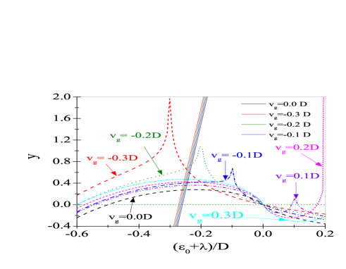
Figure 3: (color online) Determination of $\lambda$. The solid lines correspond to $y_{1}=(\tilde{\varepsilon}_{0}-\varepsilon_{0})/2\eta D-(1+v_{\text{g}}/D)$. The dashed curves are calculated from $\ln$ terms in Eq. (10). The dotted lines are grid lines. The energy unit is $D$. The other parameters are $\varepsilon_{0}=-0.3$ D, $\eta=0.02$.

We find, for $\zeta^{2}=0$,

$$\lambda=\left\{\begin{array}[]{c}\eta\left[2(D+v_{\text{g}})+\sum_{\sigma}\tilde{\varepsilon}_{0}\ln\frac{|v_{\text{g}}-\tilde{\varepsilon}_{0\sigma}|}{\tilde{\varepsilon}_{0\sigma}+D}\right],\\ \eta\left[2(D-v_{\text{g}})+\sum_{\sigma}\tilde{\varepsilon}_{0}\ln\frac{\tilde{\varepsilon}^{2}_{0}}{|\tilde{\varepsilon}_{0\sigma}+D||v_{\text{g}}-\tilde{\varepsilon}_{0\sigma}|}\right],\end{array}\right.$$ (10)

for $v_{\text{g}}+\sigma h\leq 0$, and $>0$ respectively. We solve $\lambda$ graphically, as shown in Fig. 3. The crossing points of the solid lines and the dashed lines deliver the solutions of $\lambda$ for a given gate voltage. The logarithmic terms show an interesting behaviour, the peaks being present at the positions of the gate voltages (i.e. the positions of the Fermi levels). This graph differs substantially from that discussed by Lacroix lacroix for a normal metal. A good approximate solution of $\lambda$ is inferred by replacing the renormalized impurity level in Eq. (10) with $\varepsilon_{0}$. As known, the renormalization to the energy level by the hybridization is unlikely to change the sign of the level. The occupation can not be changed by $\lambda$ alone. As a consequence, $\zeta^{2}=0$ is stable as long as $\tilde{\varepsilon}_{0\sigma}<v_{\text{g}}$. For a finite $\zeta^{2}$ we resort to numerical calculations. We derive the susceptibility (higher orders in $v_{\text{g}}$ are ignored)

$$\chi=\frac{\eta\zeta^{2}\mu^{2}_{\text{B}}}{2}\sum_{\sigma}\frac{\text{sgn}(v_{\text{g}\sigma})\left(\tilde{\varepsilon}_{0}-\eta\zeta^{2}v_{\text{g}\sigma}\right)}{(\eta\zeta^{2}\pi)^{2}v^{2}_{\text{g}\sigma}+(\tilde{\varepsilon}_{0}-v_{\text{g}\sigma}+\zeta^{2}\Re\Sigma_{\sigma})^{2}},$$ (11)

where $v_{\text{g}\sigma}=v_{\text{g}}+\sigma h$. Interestingly $\chi$ changes its sign in accordance with the sign-change of $v_{\text{g}\sigma}$ which reflects the particle-hole nature of the graphene.

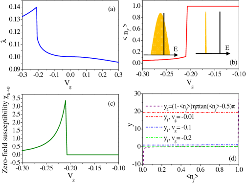
Figure 4: (color online) (a) Numerically calculated $\lambda$, (b) $\langle n_{f}\rangle$, and (c) zero field susceptibility $\chi_{h\rightarrow 0}$. (d) A graphic method to obtain the occupation by setting $\lambda=0.135$. The energy unit is $D/\pi$, $\varepsilon_{0}=-0.34$, $\eta=0.02$. The shaded regions of the insets in (b) indicate the broadened impurity level and the vertical lines indicate the positions of the Fermi level with a gate voltage. The left (right) inset corresponds to lower (higher) occupation. The function in (d) is $y_{1}=\text{sgn}(v_{\text{g}})-\tilde{\varepsilon}_{0}/|v_{\text{g}}|+(1-\langle n_{f}\rangle)\eta\text{sgn}(v_{\text{g}})\ln|\pi^{2}-v_{\text{g}}^{2}|/v_{\text{g}}^{2}$.

Figs. (4a)-(4c) show self-consistent numerical calculations demonstrating our above arguments. In Fig. (4a) $\lambda$ changes only slightly for $v_{\text{g}}>-0.1$, meaning the charge fluctuation is not large when the Fermi level does not reach the impurity level. $\lambda$ increases when a sufficient negative gate voltage is applied. However, its value can not convert the bare impurity level from negative to positive (in the local moment regime in our study). In Fig. (4b), the occupation number varies with $v_{\text{g}}$. For a small negative gate voltage, the fully occupied state is still stable, a delta-function type DOS is induced (since $\zeta^{2}\approx 0$) which is schematically shown by the right insert in Fig. (4b). When the Fermi level touches the impurity level, the charge fluctuation has a strong influence leading to a remarkable decrease in the occupation. A broadening of the impurity level occurs (linear in $v_{\text{g}}$). This strong variation in the occupation also shows up in $d$-wave superconductors zhang ; the difference to our case is that the steep decrease stems from the full occupation under insufficient gate voltage in graphene. For a comparison, in normal metals, the occupation is not complete even before the Fermi energy touches the impurity level, leading to a much smoother change hewson .

It is instructive to determine the special occupations for the varying narrow region. When $v_{\text{g}}=\tilde{\varepsilon}_{0\sigma}+\zeta^{2}\Re\Sigma_{\sigma}$, $\langle n_{f}\rangle=0.5$. When the gate voltage is lowered further, $\langle n_{f}\rangle=0.5+\frac{\Theta^{(0)}(v_{\text{g}})}{\pi}$, where $\Theta^{(0)}(v_{\text{g}})=\tan^{-1}(w(v_{\text{g}}))$ and $w(v_{\text{g}})=\frac{\text{sgn}(v_{\text{g}\sigma})}{\pi}\ln\frac{|D^{2}-v^{2}_{\text{g}\sigma}|}{v^{2}_{\text{g}\sigma}}$. In Fig. (4b), at this point, $\langle n_{f}\rangle\approx 0.4$. The $\chi_{h\rightarrow 0}$ is only nonzero when full occupation, i.e. $\langle n_{f}\rangle=1$, is violated which is shown in Fig. (4c) by a peak as lowering the gate voltage. To understand this strong change in the occupation, we derived the solutions of the occupation by the graphic method shown in Fig. (4d). The crossing points between the dashed and dash-dot lines delivers the solutions of the occupation. The tangent function is deformed by the relativestic linear dispersion to a step-like function resulting in a steep change with $v_{\text{g}}$ of the occupation, which is also comprehensible from our winding picture. Since $\zeta^{2}=0$ fixes the endpoint to $2\Theta=\pi$, the occupation can change only when the Fermi level crosses the renormalized impurity level where a sign change occurs.

V Discussions and interpretations

For a deeper insight into the step-like variation of the occupation with the gate voltage, we consider the velocity of the parameters $\lambda$ and $\langle n_{f}\rangle$ with respect to $\varepsilon_{F}$ in absence of an external magnetic field. $\lambda$ is governed by the relation

$$\lambda=\frac{\Im}{\pi}\sum_{\sigma}\int_{-D}^{\varepsilon_{F}}\frac{d\omega\Sigma_{0}}{\omega^{+}-\tilde{\varepsilon}_{0}-\zeta^{2}\Sigma_{0}}.$$ (12)

After some algebra we find that

$$\frac{\partial\lambda}{\partial\varepsilon_{F}}=\frac{(\tilde{\varepsilon}_{0}-\varepsilon_{F})\mathcal{N}_{f}(\varepsilon_{F})}{\zeta^{2}},$$ (13)

where $\mathcal{N}_{f}=\sum_{\sigma}\mathcal{N}_{f\sigma}$. The variation of the occupation with respect to $\varepsilon_{F}$ can be derived as

$$\frac{\partial\langle n_{f}\rangle}{\partial\varepsilon_{F}}=\mathcal{N}_{f}(\varepsilon_{F})=\frac{\partial\Theta(\varepsilon_{F},\lambda,\zeta^{2})}{\partial\varepsilon_{F}}.$$ (14)

From Eq. (14), we infer that the velocity of the occupation with a varying gate voltage is determined by the LDOS at the Fermi level. This velocity or LDOS also describes the curvature of the manifold $\Theta$ at the Fermi level, as interpreted in the previous section. By noting the fact that the LDOS is positive, the occupation increases with raising the gate voltage above the Dirac point. When lowering the gate voltage below the Dirac point, the occupation decreases. To know how fast the velocity of variation can be, we write explicitly

$$\mathcal{N}_{f}(\omega)=-\frac{1}{\pi}\frac{\zeta^{2}\Im\Sigma_{0}}{(\omega-\tilde{\varepsilon}_{0}-\zeta^{2}\Re\Sigma_{0})^{2}+(\zeta^{2}\Im\Sigma_{0})^{2}}.$$ (15)

When $\zeta^{2}\rightarrow 0$ ($\langle n_{f}\rangle\rightarrow 1$), the LDOS develops a delta function at the virtual impurity level. This is the case of half-filling. Therefore, if the virtual level is below the Fermi energy and a gate voltage is applied to drive the system away from the half-filling regime, the vanishing LDOS is manifested as a vanishing velocity of the occupation with the gate voltage, unless the Fermi level touches the virtual impurity energy. This is the reason for the behaviour observed in the numerical calculations. The variation of $\lambda$ with the gate voltage, From Eqs. (13) and (15), shows a maximum at $\tilde{\varepsilon}_{0}=\varepsilon_{F}$ and the restriction of $\zeta^{2}$ disappears. When the gate voltage is apart from the virtual level, $\lambda$ decreases. This can also be observed in Fig. (4a).

VI Summary

In summary, we investigated the Anderson model for a magnetic adatom above one carbon atom of one monolayer of graphene. We utilized a topological method, i.e. a degree of a map and a winding number, to analyze the occupation of the impurity and the phase shift. It is found that the phase shift is accelerated by the relativistic dispersion of graphene to complete one winding or zero winding when the impurity level is respectively below or above the Fermi energy at half-filling. The occupation varies dramatically from 1 (full occupation of the impurity) in a narrow range giving rise to a peak in the zero field susceptibility. The velocities of the renormalization of the impurity level and the occupation with respect to the gate voltage are worked out and an interpretation of the step-like variation of the occupation is provided and is consistent with the topological picture.

The work is supported by DFG and the state Saxony-Anhalt.

References

- (1) K. S. Novoselov, A. K. Geim, S. V. Morozov, D. Jiang, Y. Zhang, S. V. Dubonos, I. V. Grigorieva, and A. A. Firsov, Science 306, 666 (2004); Y. Zhang, J. P. Small, M. E. S. Amori, and P. Kim, Phys. Rev. Lett. 94, 176803 (2005); C. Berger, Z. Song, T. Li, X. Li, A. Y. Ogbazghi, R. Feng, Z. Dai, A. N. Marchenkov, E. H. Conrad, P. N. First, and W. A. de Heer, J. Phys. Chem. B 108, 19912 (2004).
- (2) A. H. Castro Neto, F. Guinea, N. M. R. Peres, K. S. Novoselov, and A. K. Geim, Rev. Mod. Phys. 81, 109 (2009).
- (3) J. C. Meyer, C. O. Girit, M. F. Crommie, and A. Zettl, Nature 454, 319 (2008); K. T. Chan, H. Lee, and M. L. Cohen, Phys. Rev. B 83, 035405 (2011).
- (4) P. S. Cornaglia, G. Usaj, and C. A. Balseiro, Phys. Rev. Lett. 102, 046801 (2009).
- (5) H. -B. Zhuang, Q. -F. Sun, and X. C. Xie, Europhys. Lett. 86, 58004 (2009).
- (6) V. N. Kotov, B. Uchoa, V. M. Pereira, A. H. Castro Neto, and F. Guinea, arXiv:1012.3484v1 [cond-mat.str-el].
- (7) B. Uchoa, V. N. Kotov, N. M. R. Peres, and A. H. Castro Neto, Phys. Rev. Lett. 101, 026805 (2008).
- (8) K. -H. Ding, Z. -G. Zhu, and J. Berakdar, J. Phys.: Condens. Matter 21, 182002 (2009).
- (9) B. Uchoa, L. Yang, S. -W. Tsai, N. M. R. Peres, and A. H. Castro Neto, Phys. Rev. Lett. 103, 206804 (2009).
- (10) M. Hentschel, and F. Guinea, Phys. Rev. B 76, 115407 (2007).
- (11) B. Dóra, and P. Thalmeier, Phys. Rev. B 76, 115435 (2007).
- (12) K. Sengupta, and G. Baskaran, Phys. Rev. B 77, 045417 (2008).
- (13) D. Jacob, and G. Kotliar, Phys. Rev. B 82, 085423 (2010).
- (14) L. Dell’Anna, J. Stat. Mech. P01007 (2010).
- (15) Z. -G. Zhu, K. -H. Ding, and J. Berakdar, Europhys. Lett. 90, 67001 (2010).
- (16) K. -H. Ding, Z. -G. Zhu, and J. Berakdar, Europhys. Lett. 88, 58001 (2009).
- (17) K. -H. Ding, Z. -G. Zhu, Z. -H. Zhang, and J. Berakdar, Phys. Rev. B 82, 155143 (2010).
- (18) D. Withoff, and E. Fradkin, Phys. Rev. Lett. 64,1835 (1990).
- (19) G. -M. Zhang, H. Hu, and L. Yu, Phys. Rev. Lett. 86,704 (2001).
- (20) B. Uchoa, T. G. Rappoport, and A. H. Castro Neto, Phys. Rev. Lett. 106, 016801 (2011).
- (21) For an exchange model (e.g., as in Ref. uchoa2011, ) when the impurity level approaches the Fermi level, usually the system enters the mixed valence regime hewson where charge fluctuations may take place where the Schrieffer-Wolff transformation schrieffer is not applicable generally.
- (22) A. C. Hewson, The Kondo problem to heavy fermions, (Cambridge Uni. Press, 1993).
- (23) As discussed in Ref. hewson , the -variation of the selfenergy does not contribute to the integral that determines .
- (24) J. R. Schrieffer, and P. A. Wolff, Phys. Rev. 149, 491 (1966).
- (25) P. Coleman, Phys. Rev. B 29, 3035 (1984).
- (26) B. A. Dubrovin, A. T. Fomenko, and S. P. Novikov, Modern geometry-methods and applications: part II. The geometry and topology of manifolds, (Springer-Verlag New York Inc. 1985).
- (27) C. Lacroix, J. Phys. F: Metal Phys. 11, 2389 (1981).