A robust sample of galaxies at redshifts $\mn@boldsymbol{6.0<z<8.7}$:
stellar populations, star-formation rates and stellar masses

Abstract

We present the results of a photometric redshift analysis designed to identify redshift $z\geq 6$ galaxies from the near-IR HST imaging in three deep fields (HUDF, HUDF09-2 & ERS) covering a total area of 45 sq. arcmin. By adopting a rigorous set of criteria for rejecting low-redshift interlopers, and by employing a deconfusion technique to allow the available ultra-deep IRAC imaging to be included in the candidate selection process, we have derived a robust sample of 70 Lyman-break galaxies (LBGs) spanning the redshift range $6.0<z<8.7$. Based on our final sample we investigate the distribution of UV spectral slopes ($f_{\lambda}\propto\lambda^{\beta}$), finding a variance-weighted mean value of $\langle\beta\rangle=-2.05\pm 0.09$ which, contrary to some previous results, is not significantly bluer than displayed by lower-redshift starburst galaxies. We confirm the correlation between UV luminosity and stellar mass reported elsewhere, but based on fitting galaxy templates featuring a range of star-formation histories, metallicities and reddening we find that, at $z\geq 6$, the range in mass-to-light ratio ($M_{\star}/L_{\rm UV}$) at a given UV luminosity could span a factor of $\simeq 50$. Focusing on a sub-sample of twenty-one candidates with IRAC detections at $3.6\mu$m we find that $L^{\star}$ LBGs at $z\simeq 6.5$ have a median stellar mass of $M_{\star}=(2.1\pm 1.1)\times 10^{9}\hbox{$\rm\thinspace M_{\odot}$}$ (Chabrier IMF) and a median specific star-formation rate (sSFR) of $1.9\pm{0.8}$ Gyr^-1. Using the same sub-sample we have investigated the influence of nebular continuum and line emission, finding that for the majority of candidates (16 out of 21) the best-fitting stellar masses are reduced by less than a factor of 2.5. However, galaxy template fits exploring a plausible range of star-formation histories and metallicities provide no compelling evidence of a clear connection between star-formation rate and stellar mass at these redshifts. Finally, a detailed comparison of our final sample with the results of previous studies suggests that, at faint magnitudes, several high-redshift galaxy samples in the literature are significantly contaminated by low-redshift interlopers.

1 INTRODUCTION

The goal of identifying and studying the nature of ultra high-redshift galaxies remains one of the most important challenges in observational cosmology, and holds the key to furthering our understanding of the earliest stages of galaxy evolution and unveiling the nature of the sources responsible for cosmic reionization.

Observational constraints provided by the Gunn-Peterson trough in the spectra of high-redshift quasars (e.g Fan et al. 2006) suggest that reionization was coming to an end at $z\simeq 6$ (Becker et al. 2007). Moreover, optical polarization measurements from the WMAP experiment indicate that reionization began at $z\simeq 11$ if it is assumed to be a single, rapid event (Dunkley et al. 2009). Consequently, it is now apparent that to improve our understanding of cosmic reionization, and to unveil the earliest epoch of galaxy formation, it is necessary to extend studies of high-redshift galaxies into the redshift $7<z<10$ régime (e.g. Robertson et al. 2010).

Given our existing knowledge of the evolution of the galaxy luminosity function in the redshift interval $5.0<z<6.5$ (e.g. Bouwens et al. 2007; McLure et al. 2009) it is clear that achieving this aim requires ultra-deep near-IR imaging, reaching detection limits of $26<m_{AB}<30$. At the bright end of this range, wide-field, ground-based imaging has a unique contribution to make, and has recently allowed the luminosity function, the clustering properties and the stellar populations of luminous Lyman-break galaxies (LBGs: McLure et al. 2009; Ouchi et al. 2009; Grazian et al. 2010) and Lyman alpha emitters (LAEs: Ouchi et al. 2010; Ota et al. 2010; Ono et al. 2010; Nakamura et al. 2010) to be studied in detail. Indeed, the importance of ground-based imaging and spectroscopy has recently been highlighted by the spectroscopic confirmation of two LBGs at $z=7.01$ and $z=7.11$ by Vanzella et al. (2010). However, in advance of 30-m class ground-based telescopes, it is clear that routinely identifying and studying sub-L^⋆ galaxies at $z\geq 7$ is only possible using space-based imaging.

Consequently, the unparalleled near-IR sensitivity provided by the new WFC3 camera, installed on the Hubble Space Telescope (HST) in late 2009, has proven to be a crucial breakthrough in high-redshift galaxy studies. Indeed, despite only covering an area of $\simeq 4.5$ sq. arcmin, the unprecedented depth ($m_{AB}\simeq 29$, $5\sigma$) of the first tranche of WFC3/IR imaging of the Hubble Ultra Deep Field (HUDF; GO-11563) led to a raft of early science papers investigating the number densities, luminosity functions, stellar masses and stellar populations of $6.5<z<8.5$ galaxies (e.g. Bouwens et al. 2010ab; Oesch et al. 2010; McLure et al. 2010; Yan et al. 2010; Labbé et al. 2010; Finkelstein et al. 2010; Bunker et al. 2010). Interestingly, Lehnert et al. (2010) have recently claimed the tentative detection of Ly$\alpha$ emission at $z=8.56$ in a WFC3/IR candidate in the HUDF, originally identified by Bouwens et al. (2010a) and McLure et al. (2010). Although the large rest-frame equivalent width (EW$\simeq 210$Å) of the Ly$\alpha$ emission line suggests that, if confirmed, this object must be a decidedly atypical example of a $z\geq 6$ LBG (Stark, Ellis & Ouchi 2010), the location of the claimed Ly$\alpha$ emission line is in good agreement with the original photometric redshifts derived by McLure et al. (2010) and Finkelstein et al. (2010); $z_{phot}=8.45\pm 0.50$ and $z_{phot}=8.61\pm{0.35}$ respectively.

In addition to the WFC3/IR imaging of the HUDF, another key dataset has been the WFC3/IR imaging taken as part of the Early Release Science extra-galactic programme (ERS; GO-11359) which, although substantially shallower than the HUDF WFC3/IR imaging ($m_{AB}\simeq 27.5$, $5\sigma$), covers an area approximately ten times larger. By combining the HUDF and ERS datasets to obtain greater dynamic range in UV luminosity, Bouwens et al. (2010b) and Labbé et al. (2010) investigated the relationship between the UV spectral slope ($f_{\lambda}\propto\lambda^{\beta}$) and UV luminosity. Both studies find a correlation, with $\beta$ changing from $\beta\simeq-2$ (a typical value for lower-redshift starburst galaxies) at $M_{1500}\simeq-20.5$, to extremely blue values of $\beta\simeq-3$ at $M_{1500}\simeq-18.5$. As discussed by Bouwens et al. (2010b), although dust-free, low metallicity models can produce slopes of $\beta\simeq-3$, they can only do so under the assumption that the ionising photon escape fraction is high ($f_{esc}>0.3$) and that, correspondingly, the contribution from nebular continuum emission is low.

Based on stacking the ACS+WFC3/IR+IRAC photometry of $z\simeq 7$ LBG candidates in the HUDF and ERS datasets, Labbé et al (2010) find the same correlation between $M_{1500}$ and spectral slope $\beta$ as Bouwens et al. (2010b). However, Labbé et al. (2010) conclude that it is not possible to reproduce both the blue spectral slopes and significant $\lambda_{rest}\simeq 4000$Å  spectral breaks displayed by the faintest $z\simeq 7$ LBG candidates, without recourse to episodic starformation histories and/or a significant contribution from nebular line emission. Indeed, Ono et al. (2010) also conclude that nebular line emission may be necessary to reproduce the observed $J-$m_3.6 colour in a stack of $z\simeq 6$ LAE photometry.

Despite the uncertainties, one observational result that has received significant attention recently is the apparent relationship between star-formation rate and stellar mass. Both Labbé et al. (2010) and González et al. (2010) find an approximately linear correlation between stellar mass and star-formation rate at $z\simeq 7$, consistent with the results derived by Stark et al. (2009) for LBGs in the redshift range $4<z<6$. As a result, Labbé et al (2010) and González et al. (2010) conclude that the specific star-formation rate (sSFR) of $z\simeq 7$ LBGs is remarkably constant (sSFR $\simeq 2$ Gyr^-1), and consistent with the value of sSFR $\simeq 2.5-4.5$ Gyr^-1 observed in star-forming galaxies at $z\simeq 2-3$ (e.g. Daddi et al. 2007; Magdis et al. 2011). As previously discussed by Stark et al. (2009), a natural explanation of this observation would be to invoke a star-formation rate which exponentially increases with time although, as shown by Finlator, Oppenheimer & Davé (2011), star-formation histories of this type may have difficulty in reproducing some of the most extreme Balmer breaks reported in the literature at $z\geq 6$.

The majority of previous studies which have investigated the high-redshift galaxy population using WFC3/IR imaging have relied on traditional colour-cut, or “drop-out”, selection techniques. In contrast, the principal motivation for this paper is to investigate what can be learned about the $z\geq 6$ galaxy population by fully exploiting the excellent multi-wavelength (ACS+WFC3/IR+IRAC) data which is now available over an area of $\simeq 45$ sq. arcmin. Rather than applying standard “drop-out” criteria, in this work we continue to pursue the strategy we have previously adopted (McLure et al. 2006; 2009; 2010) and employ a template-fitting, photometric redshift analysis to select our final high-redshift galaxy sample. A key new element in this strategy is our development of a deconfusion algorithm capable of providing the robust IRAC photometry necessary for improved photometric redshift and stellar-mass estimates.

In principle this technique should have several advantages over the standard LBG “drop-out” selection. Firstly, by employing all of the available multi-wavelength data, including the IRAC photometry, it is possible to make optimal use of the available information. Secondly, by avoiding any colour pre-selection this approach should be less biased towards simply selecting the very bluest galaxies at high-redshift. This second point is potentially crucial within the context of investigating the claims of ultra-blue UV spectral slopes for LBG candidates at $z\geq 6$ (see Section 4). Finally, an SED fitting analysis also provides an estimate of the photometric redshift probability density function, $P(z)$, and therefore allows the prevalence, and significance, of competing photometric redshift solutions at low redshift to be transparently investigated.

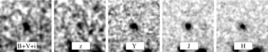
The primary motivation of this paper is therefore to construct the most robust sample possible using the available data and techniques reviewed above, in order to critically address some of the claims about the properties of the $z>6$ population newly-found with HST. The structure of the paper is as follows. In Section 2 we describe the available data in each of the three fields, including a brief description of our IRAC deconfusion algorithm. In Section 3 we describe our initial candidate selection, photometric redshift analysis and the construction of the final catalogue of robust candidates. In Sections 4 and 5 we investigate the UV spectral slopes, stellar masses and star-formation rates of the final robust sample. In Section 6 we perform a detailed comparison of our final robust sample with samples previously derived in the literature, exploring the reasons behind any apparent discrepancies. In Section 7 we provide a summary of our main conclusions. In the Appendix we provide a full description of our IRAC deconfusion procedure, full photometry and grey-scale postage stamp images for each high-redshift candidate and individual plots illustrating the results of our SED fitting. All magnitudes are quoted in the AB system (Oke & Gunn 1983) and all calculations assume $\Omega_{0}=0.3,\Omega_{\Lambda}=0.7$ and $H_{0}=70$ kms^-1Mpc^-1.

2 DATA

The analysis in this paper relies on the publicly available optical, near-IR and mid-IR imaging data covering the HUDF, HUDF09-2 and ERS fields. In this section we briefly describe the relevant details of the various imaging datasets, and the depth analysis which was performed in order to attribute accurate error estimates to the candidate photometry. The basic properties of the three fields are listed in Table 1.

Figure 1: Illustration of the IRAC deconfusion algorithm. The left-hand panel shows the inverse-variance weighted stack of the epoch1+epoch2 $4.5\mu$m imaging covering the HUDF. The middle panel shows the best-fitting model of the IRAC data, based on using the $H_{160}$ WFC3/IR imaging to provide model templates, and a matrix inversion procedure to determine the best-fitting template amplitudes (see Appendix A for full details). The right-hand panel shows the model subtracted image (note that the WFC3/IR imaging does not cover the full area of the HUDF).

2.1 WFC3/IR imaging

The WFC3/IR imaging of both the HUDF and the HUDF09-2 fields was taken as part of the public treasury programme GO-11563 (P.I.=Illingworth) and consists of single pointings ($\simeq 4.5$ sq. arcmin) of the WFC3/IR camera in the F105W, F125W and F160W filters (hereafter referred to as $Y_{105},J_{125}$ and $H_{160}$). The WFC3/IR dataset in the ERS field was taken as part of the public programme GO-11359 (P.I.=O’Connell) and consists of a mosaic of 10 pointings of the WFC3/IR camera in the F098M ($Y_{098}$), $J_{125}$ and $H_{160}$ filters (Windhorst et al. 2011) . The WFC3/IR data were calibrated using calwf3 and subsequently combined using MultiDrizzle (Koekemoer et al. 2002) as summarized in McLure et al. 2010); full details are presented in Koekemoer et al. (2011). The final mosaics have PSFs with FWHM in the range $0.15$^′′$-0.18$^′′depending on the filter, and were drizzled onto a final grid of 0.06^′′/pix. In the case of the HUDF and ERS mosaics, the final astrometry was matched to that of the publicly available reductions of the optical ACS imaging of the UDF (Beckwith et al. 2006) and GOODS-S (GOODSv2.0; Giavalisco et al. 2004) respectively. The astrometry for the final mosaics of the HUDF09-2 field was matched to the $J-$band imaging of GOODS-S taken as part of the MUSYC survey (Cardamone et al. 2010), with a typical r.m.s. accuracy of $\simeq 0.1$^′′. The WFC3/IR imaging of the ERS analysed in this paper consists of the data comprising the completed programme. However, for the HUDF09-2 and HUDF fields we make use of the epoch 1 observations, which consist of the data publicly available as of February 2010 and August 2010 respectively.

2.2 ACS imaging

For the HUDF and ERS fields the ACS data used in this study consists of the publicly available reductions of the F435W, F606W, F775W and F850LP (hereafter $B_{435},V_{606}$, $i_{775}$ and $z_{850}$) imaging of the HUDF (Beckwith et al. 2006) and GOODS-S (v2.0; Giavalisco et al. 2004). The ACS imaging covering the HUDF09-2 field is our own reduction (based on calacs and MultiDrizzle) of the $V_{606},i_{775}$ and $z_{850}$ imaging obtained as part of the UDF05 programme (Oesch et al. 2007). All of the optical ACS imaging was re-sampled to a 0.06^′′/pix grid to match the WFC3/IR data, and the astrometry of the ACS data covering HUDF09-2 was also registered to match the MUSYC imaging of GOODS-S.

2.3 IRAC imaging

For the HUDF and ERS fields we make use of the publicly available reductions (v0.30) of the $3.6\mu$m and $4.5\mu$m IRAC imaging obtained as part of the GOODS survey (proposal ID 194, Dickinson et al.; in preparation). The IRAC data covering the ERS consists of approximately 23 hours of on-source integration in both the $3.6\mu$m and $4.5\mu$m bands. For the HUDF we performed an inverse variance weighted stack of the overlapping region of the epoch 1 and epoch 2 imaging, producing final mosaics consisting of approximately 46 hours of on-source integration at $3.6\mu$m and $4.5\mu$m. For the HUDF09-2 we re-registered and stacked the mopex reductions of the $3.6\mu$m imaging obtained via proposal ID 30866 (P.I. R. Bouwens) producing a final $3.6\mu$m mosaic with an on-source integration time of approximately 33 hours. The consistency of the IRAC photometry was checked via reference to the SIMPLE (Damen et al. 2010) imaging at $3.6\mu$m and $4.5\mu$m of the E-CDFS, which overlaps all three fields. The astrometry of the IRAC imaging in all three fields was registered to that of the corresponding $H_{160}$ WFC3/IR imaging.

2.3.1 IRAC deconfusion

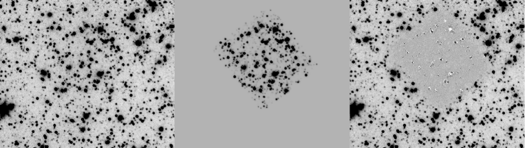
A key new feature of the analysis undertaken in this paper is the inclusion of the IRAC photometry in the candidate high-redshift galaxy selection procedure. Due to its depth, and comparatively broad PSF (FWHM $\simeq 1.5$^′′), the $3.6+4.5\mu$m IRAC imaging covering the three fields of interest is heavily confused, making the process of obtaining aperture photometry matched to the optical/nearIR HST imaging non trivial. In order to achieve this aim it is therefore necessary to pursue some form of deconfusion process, which allows the IRAC imaging to be utilised beyond the natural confusion limit. Although there are several techniques which can be used to deconfuse IRAC imaging (see Appendix A) we have developed our own software which uses the WFC3/IR imaging data to provide normalized templates for each object in the field and then, via a transfer function, produces synthetic IRAC images on the native 0.6^′′/pix plate scale. Through a matrix inversion procedure, the amplitude (or total flux) of each template can be simultaneously fitted to produce the optimal reproduction of the observed IRAC image (see Fig. 1). As a result of this procedure it is effectively possible to extract accurate aperture photometry from the $3.6\mu$m and $4.5\mu$m IRAC imaging at the spatial resolution of the WFC3/IR imaging. An additional advantage of this approach is that it naturally provides robust uncertainties on the delivered flux measurements, which depend both on the signal-to-noise ratio of the IRAC detection and the local level of confusion in the IRAC image.

Figure 2: Example plots showing the results of our SED-fitting for three objects from our final robust sample at redshifts $z_{phot}~{}=~{}6.5,7.0\,\&\,8.7$ (top to bottom). In each plot the thick (blue) line shows the best-fitting high-redshift galaxy template, and the thin dotted (red) line shows the best-fitting alternative solution at low redshift. In each panel the inset shows the value of $\chi^{2}$ as a function of redshift (marginalized over all other free parameters). The horizontal line in each inset panel highlights the location of ($\chi^{2}_{min}+4$) which corresponds to our requirement that a candidate is considered “robust” only if any alternative low-redshift solutions can be ruled-out at the $\geq 95\%$ confidence level. In each example, the combination of image depth and wavelength coverage allows us to rule-out any alternative low-redshift solutions with high confidence. The bottom panel (HUDF09-2$\_2765$) provides a good example of a situation where even a robust upper limit to the IRAC $3.6\mu$m flux provides a powerful redshift discriminant.

Table 1: The results of the image depth analysis described in Section 3.2. Columns 1-4 list the survey field names, central coordinates and areas (in sq. arcmin). The areas listed in column 4 correspond to the areas of WFC3/IR imaging which were actually useful for the analysis performed in this paper (i.e excluding array edges and areas which are not covered by ACS optical imaging). The remaining columns list the median $5\sigma$ depths in each available ACS+WFC3/IR+IRAC filter. The depths are all referenced to a 0.6^′′diameter aperture, and are not aperture corrected. Due to the fact that the IRAC depths are determined via a deconfusion process (see Section 2.3.1), the local IRAC depths can differ significantly from the median values listed here.

Field	RA(J2000)	DEC(J2000)	Area	$B_{435}$	$V_{606}$	$i_{775}$	$z_{850}$	$Y_{098}$	$Y_{105}$	$J_{125}$	$H_{160}$	$3.6\mu$m	$4.5\mu$m
HUDF	03:32:38.5	$-27$:46:57.0	4.5	29.04	29.52	29.19	28.54	$-$	28.59	28.67	28.73	26.3	25.9
HUDF09-2	03:32:23.4	$-27$:42:52.0	4.5	$-$	28.49	28.22	28.06	$-$	28.24	28.60	28.49	26.2	$-$
ERS	03:33:05.5	$-27$:51:21.6	36.5	27.68	27.87	27.29	27.06	27.26	$-$	27.66	27.40	26.0	25.6

3 Candidate selection

The process of candidate selection can be broken down into three separate stages: object detection and photometry, photometric redshift analysis and sample cleaning. Each stage in the process is described below.

3.1 Object detection and photometry

The initial catalog construction process was identical in each of the three fields, and relied on sextractor v2.5.0 (Bertin et al. 1996). Preliminary catalogues were constructed in which object detection was performed in the $Y_{105W}/Y_{098M}$, $J_{125W}$ and $H_{160W}$ bands, using an aggressive set of sextractor parameters, with matched photometry extracted from the corresponding ACS imaging by running sextractor in dual image mode. The separate catalogues were then concatenated to produce a master catalog of unique objects in each of the three fields.

In order to avoid biases which can be introduced by adopting small photometric apertures, all of the analysis in this paper is based on 0.6^′′diameter aperture photometry. For the purposes of the photometric redshift analysis, the fluxes from the 0.6^′′diameter aperture photometry are not corrected to total, but the WFC3/IR and IRAC fluxes are corrected by small amounts (2%-10%) to account for aperture losses relative to the ACS imaging.

3.2 Depth Analysis

A crucial part of the analysis necessary to identify robust high-redshift candidates is the derivation of accurate photometric uncertainties in each band. This was achieved by first producing a so-called $\chi^{2}$ image (Szalay, Connolly & Szokoly 1999) of the registered optical+nearIR images of each field to identify which pixels are genuine “blank sky”. Secondly, a grid of 0.6^′′diameter apertures was placed in the blank sky regions on each image. Thirdly, in order to determine the local image depth for each candidate, in each filter, the r.m.s. aperture-to-aperture variation was determined, by examining the distribution of the nearest 50 blank apertures. In this fashion, we are able to determine a local depth measurement for each individual candidate. For information, the median $5\sigma$ depths for each field are listed in Table 1.

3.3 Photometric redshift analysis

To perform the SED analysis necessary for this study we have developed a new, bespoke, template-fitting code. The primary motivation for developing this new code was to provide the freedom to explore the relevant multi-dimensional parameter space in detail, investigating the impact of different SED templates, IMFs, dust attenuation prescriptions and IGM absorption recipes. Moreover, by employing our own software it is possible to have full control over which derived quantities are provided as output, and the exact details of how the template fitting is performed. For example, our new code performs the SED fitting based on flux densities ($f_{\nu}$), rather than magnitudes, which has the advantage of allowing the flux errors to be dealt with in a rigorous manner. Moreover, if necessary, the new code offers the possibility of fitting the input photometry with multi-component stellar populations, each with separate metallicities and/or dust attenuation prescriptions.

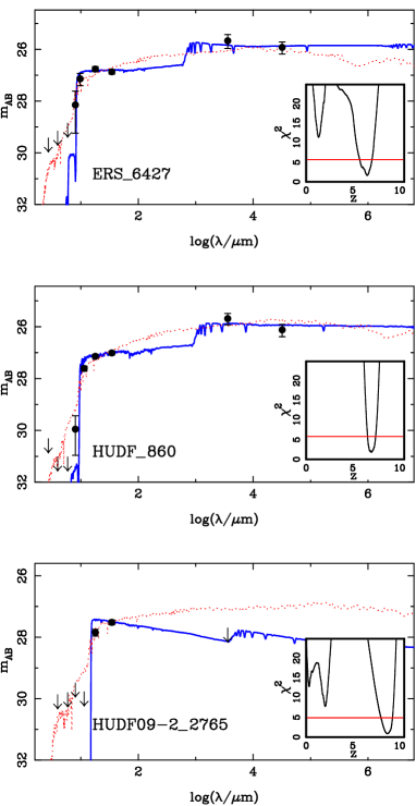
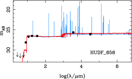
For the purposes of this study we employed the Bruzual & Charlot (2003) and Charlot & Bruzual 2007 (priv. comm) stellar evolution models (hereafter BC03 & CB07), considering models with metallicities ranging from solar ($Z_{\odot}$) to $1/50$th solar ($0.02Z_{\odot}$). Models with instantaneous bursts of star-formation, constant star-formation and star-formation rates exponentially declining with characteristic timescales in the range 50 Myrs $<~{}\tau~{}<$ 10 Gyrs were all considered. The ages of the stellar population models were allowed to range from 10 Myrs to 13.7 Gyrs, but were required to be less than the age of the Universe at each redshift. Dust reddening was described by the Calzetti et al. (2003) attenuation law, and allowed to vary within the range $0.0<A_{V}<2.5$ magnitudes. Inter-galactic medium absorption short-ward of Ly$\alpha$ was described by the Madau et al. (1995) prescription, and a Chabrier (2003) IMF was assumed in all cases . In Fig. 2 we show example SED fits for three objects (one from each field) covering the redshift range $6.5<z_{phot}<8.7$.

3.4 Sample cleaning

Based on the results of the photometric redshift fitting, all objects which displayed a statistically acceptable solution at $z_{phot}\geq 4.5$ were retained, while those with no acceptable solution at high redshift were excluded. In each of the three fields, this initial screening process removed more than 90% of the original input catalogues. Following the initial photometric redshift fitting, the remaining samples of potential high-redshift candidates were manually screened to remove artefacts (e.g. diffraction spikes), edge effects and spurious candidates such as high-surface brightness features within the extended envelopes of luminous low-redshift galaxies.

Figure 3: In black we show the redshift distribution of our final robust sample, which has been calculated by summing the estimated redshift probability density function of each candidate. This is our best estimate of the redshift distribution of the N=70 objects which satisfy all three of the criteria listed in Section 3.4.1. In grey we show the redshift distribution of the N=130 objects which satisfy the first criterion listed in Section 3.4.1 (i.e. a statistically acceptable redshift solution at $z_{phot}\geq 6.0$) but fail the other two criteria (see text for details).

3.4.1 Final candidate sample

From a practical perspective, the primary goal of this study is to produce a robust sample of high-redshift galaxy candidates at $z~{}\geq~{}6$. In order to achieve this aim, three criteria were applied to the remaining potential high-redshift candidates:

• Statistically acceptable redshift solution at $z_{phot}\geq 6.0$

• Secondary redshift solution excluded at $\geq 95\%$ confidence

• Integrated probability $\int^{z=10}_{z=6}P(z^{\prime})\delta z^{\prime}\geq 0.5$

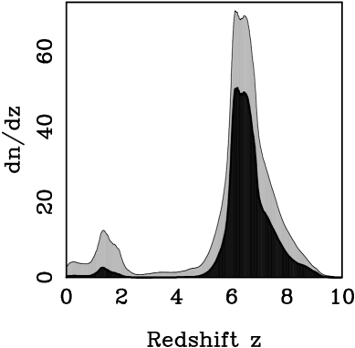
The first criterion simply restricts our final sample to those objects for which the best-fitting SED template lies at $z_{phot}\geq 6$. The second criterion rejects those objects for which the competing low-redshift solution cannot be excluded at high confidence. Specifically, this criterion is enforced by insisting that the $\Delta\chi^{2}$ between the primary and secondary photometric redshift solution (following marginalization over all other relevant parameters) is $\Delta\chi^{2}\geq 4$. The final criterion is designed to exclude a small number of candidates with relatively flat $P(z)$ distributions for which, despite having a primary photometric redshift solution at $z_{phot}\geq 6$, the majority of their integrated probability density distribution function lies at $z_{phot}\leq 6$. We note that this final criterion is very similar to that employed by Finkelstein et al. (2010) in their HUDF analysis.

Our final robust sample of $z\geq 6$ galaxy candidates consists of N=70 objects, spanning the redshift range $6.0<z<8.7$ and covering more than a factor of ten in intrinsic UV luminosity, from $-18.2<M_{1500}<-21.2$ . It is perhaps worth pointing out that if we had only insisted on a statistically acceptable primary photometric redshift solution at $z_{phot}\geq 6.0$, the final sample would contain N=130 candidates. It should be stressed that it is likely that a significant fraction of the excluded objects are indeed $z\geq 6$ galaxies (see Fig. 3), it is simply that with the data in-hand, it is not possible to consider them as robust candidates.

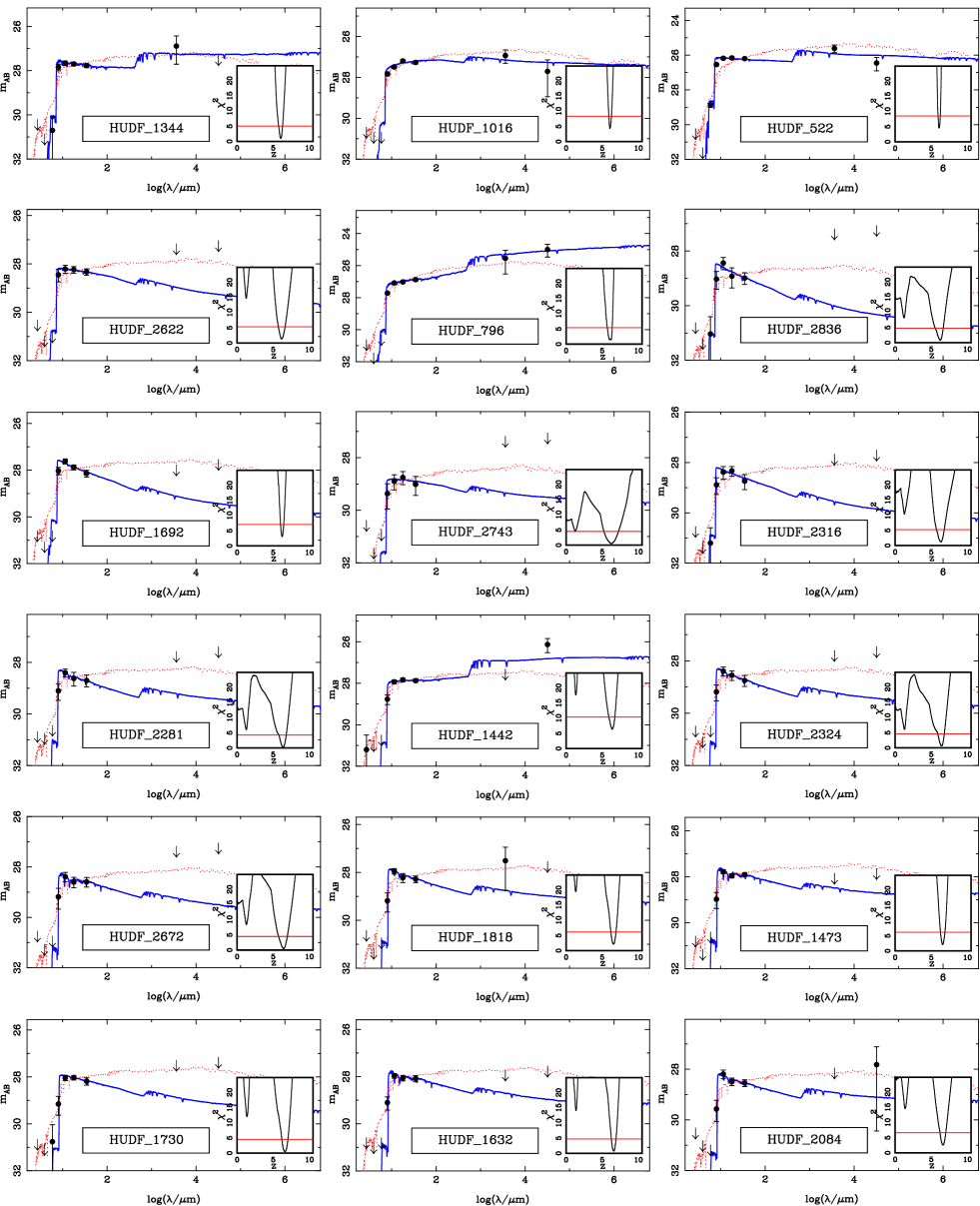
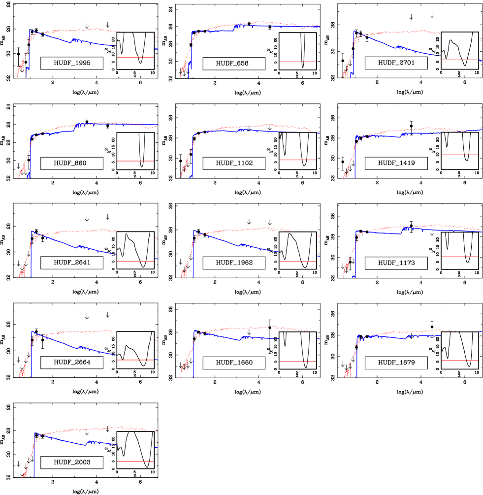
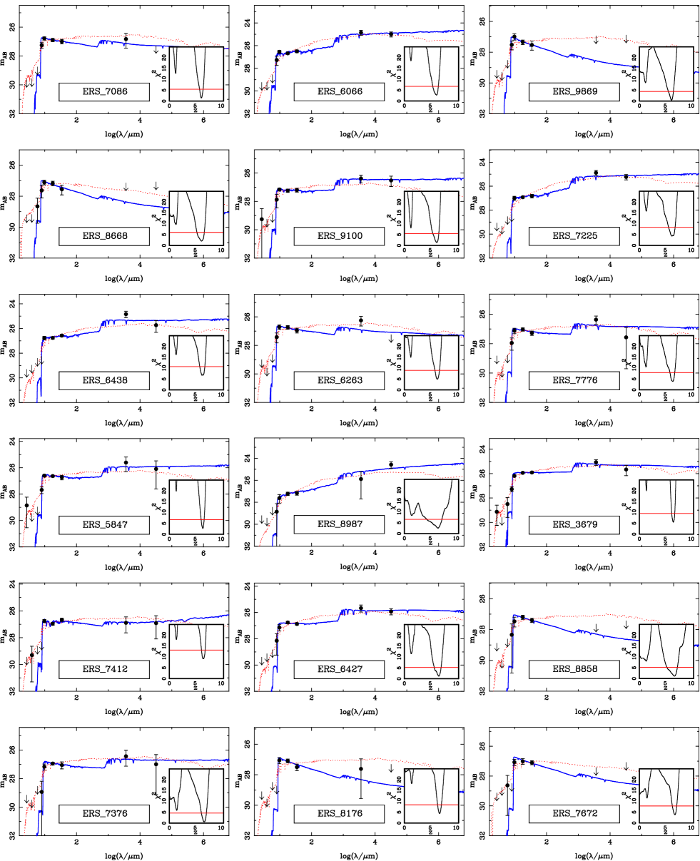
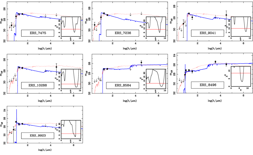
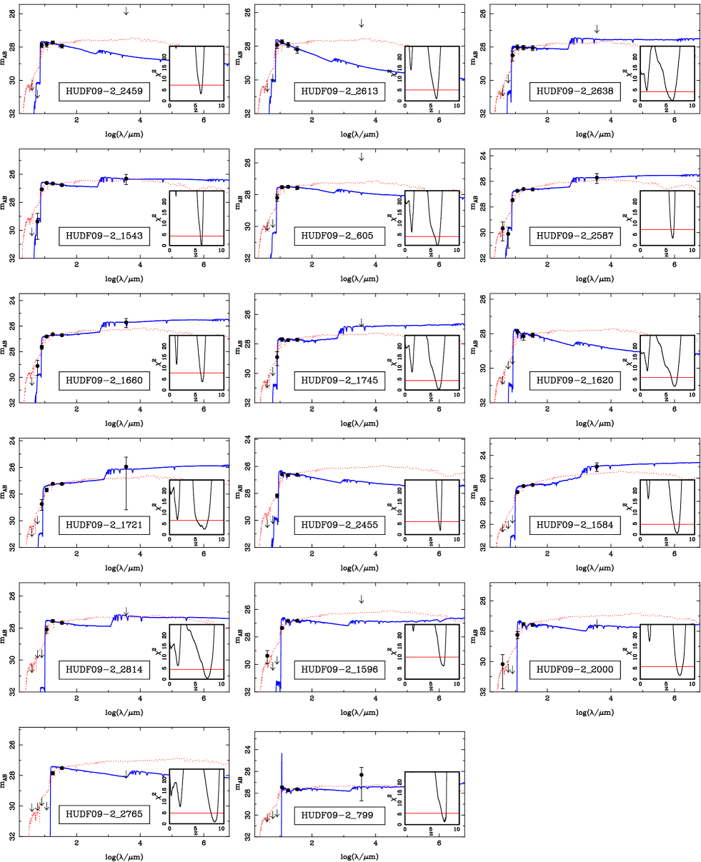
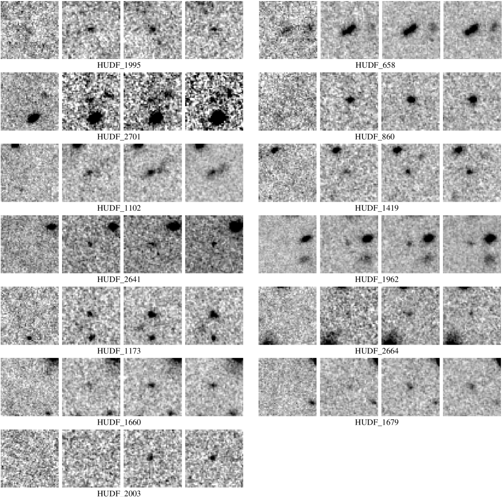
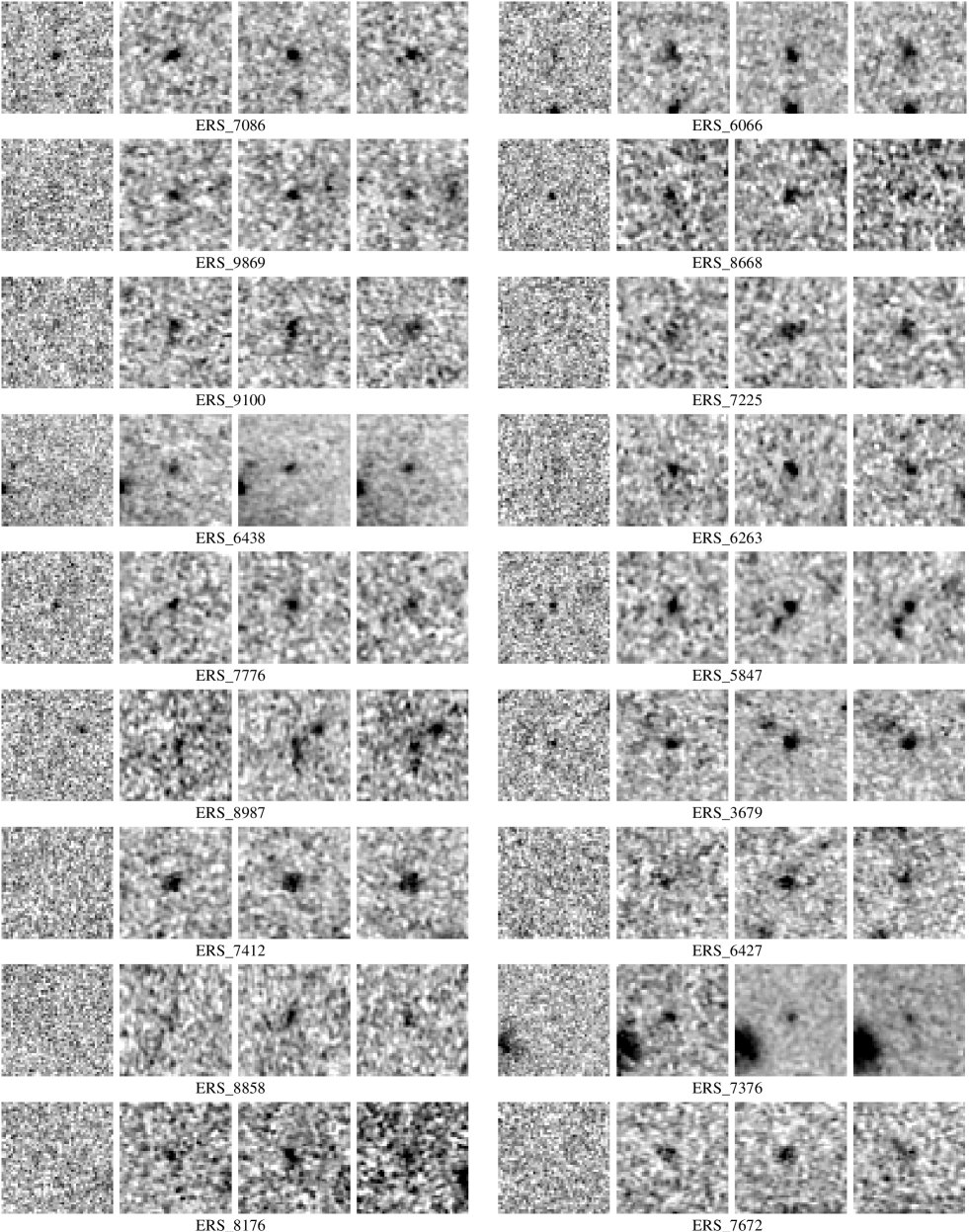
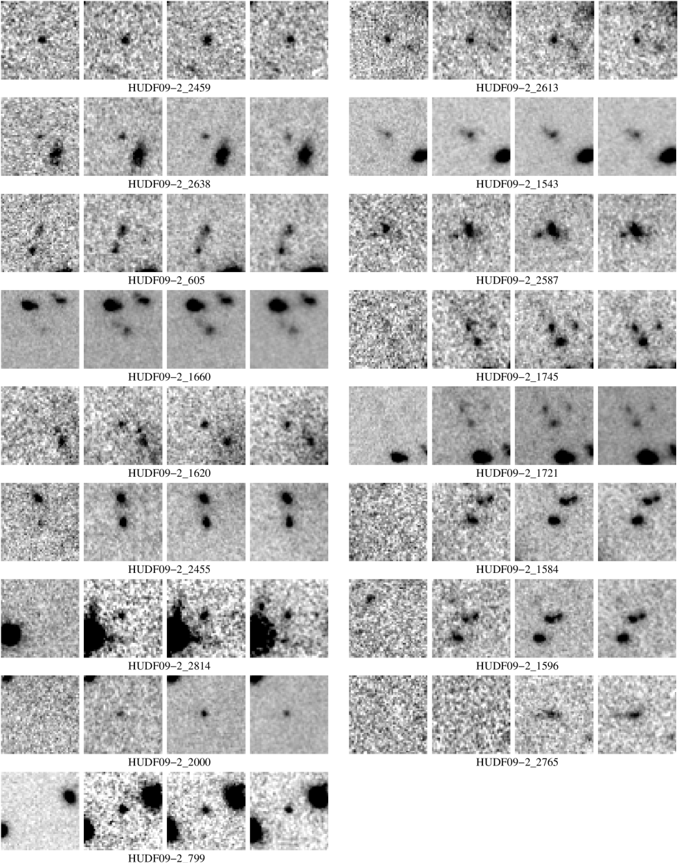
Due to the fact that LBGs at $z\geq 6$ are necessarily young galaxies, the differences between the SED fits provided by the BC03 and CB07 models are negligible. Consequently, to ease the comparison with previous studies, throughout the rest of the paper we adopt the results of the SED-fitting analysis based on the BC03 models. The final robust samples in each of the three fields, along with the best-fitting photometric redshift solutions and various other derived parameters are presented in Tables 2, 3 & 4. Note that, although we make no further use of this information throughout the rest of the paper, in Tables 2, 3 & 4 we also list the best-fitting photometric redshift for each candidate if Ly$\alpha$ emission with a rest-frame EW₀ in the range 0Å $<$ EW${}_{0}<$ 240Å  is included as an extra free parameter in the SED-fitting procedure. This information is provided to indicate the maximum plausible redshift for each candidate. The three candidates which are listed separately at the bottom of Tables 3 & 4 only pass our criteria as robust $z\geq 6$ candidates if Ly$\alpha$ emission is included in the SED-fitting procedure, and are not included in any of the subsequent analysis. The 0.6^′′diameter aperture photometry for each candidate is listed in Tables B1, B2 & B3 of Appendix B, along with plots of the best-fitting SED templates and grey-scale optical-nearIR postage stamps.

Figure 4: Plots of UV spectral slope ($\beta$) versus redshift for the final robust sample of seventy objects at $z_{phot}\geq 6$. The top three panels show $\beta$ versus redshift for the three separate survey fields, while the bottom panel shows $\beta$ versus redshift for the full combined sample. In each panel the horizontal line shows the variance-weighted mean value of $\beta$ (see Table 5).

Table 2: Details of the final high-redshift sample in the HUDF field. The first three columns list the ID number and coordinates of each candidate. Columns four, five and six list the photometric redshifts, the $1\sigma$ uncertainty on the photometric redshifts and the values of $\chi^{2}$ for the best-fitting SED template. Column seven lists the difference in $\chi^{2}$ between the best-fitting high-redshift SED template and the alternative photometric redshift solution at low redshift (typically at $1.0<z_{phot}<2.5$). Column eight lists the absolute magnitude of the best-fitting SED template, where $M_{1500}$ is measured using a 100Å -wide filter centred on a rest-frame wavelength of 1500Å. Column nine lists the value of the UV spectral slope ($f_{\lambda}\propto\lambda^{\beta})$ for each candidate, derived using the formulae listed in Section 4. Column ten lists the best-fitting photometric redshift derived including Ly$\alpha$ emission as an additional free parameter, and column eleven lists the logarithm of luminosity of the corresponding best-fitting Ly$\alpha$ emission line (in ergs s^-1). Column twelve lists the results of cross-checking each candidate against existing literature studies of the WFC3/IR data in the HUDF field. Matches were found with the following papers: M (McLure et al. 2010); B (Bouwens et al. 2011; robust), Bp (Bouwens et al. 2011; potential), F (Finkelstein et al. 2010), W (Wilkins et al. 2010), Y (Yan et al. 2010) and L (Lorenzoni et al. 2011).

ID	RA(J2000)	DEC(J2000)	z	$\Delta z$	$\chi^{2}$	$\Delta\chi^{2}$	M1500	$\beta$	zLyα	$\log(L_{Ly\alpha})$	Literature
HUDF_1344	03:32:36.63	$-27$:47:50.1	6.06	5.89$-$6.17	1.1	27.6	$-19.3$	$-2.2\pm 0.7$	6.16	42.2	M
HUDF_1016	03:32:35.06	$-27$:47:40.2	6.06	5.97$-$6.15	4.3	32.0	$-19.6$	$-0.4\pm 0.6$	6.33	42.4	M
HUDF_522	03:32:36.47	$-27$:46:41.4	6.07	5.98$-$6.15	4.5	151.3	$-20.8$	$-1.9\pm 0.6$	6.07	$-$	$-$
HUDF_2622	03:32:36.64	$-27$:47:50.2	6.11	5.95$-$6.38	1.3	13.4	$-18.8$	$-2.2\pm 1.2$	6.43	42.3	M
HUDF_796	03:32:37.46	$-27$:46:32.8	6.19	5.86$-$6.31	1.4	46.0	$-19.9$	$-1.7\pm 0.6$	6.50	42.7	M,F
HUDF_2836	03:32:35.05	$-27$:47:25.8	6.22	5.97$-$6.43	0.8	7.4	$-18.4$	$-4.6\pm 2.3$	6.51	42.1	M
HUDF_1692	03:32:43.03	$-27$:46:23.6	6.23	6.11$-$6.34	3.1	38.5	$-19.3$	$-3.4\pm 0.8$	6.49	42.4	M
HUDF_2743	03:32:36.52	$-27$:46:42.0	6.26	5.80$-$6.72	0.5	4.0	$-18.2$	$-1.2\pm 2.0$	6.40	41.7	M,Y
HUDF_2316	03:32:44.31	$-27$:46:45.2	6.31	6.03$-$6.54	1.2	9.1	$-18.7$	$-1.7\pm 1.7$	6.30	$-$	M
HUDF_2281	03:32:39.79	$-27$:46:33.7	6.37	6.11$-$6.57	0.3	5.7	$-18.6$	$-3.2\pm 1.7$	6.35	$-$	M
HUDF_1442	03:32:42.19	$-27$:46:27.8	6.37	6.17$-$6.55	6.4	11.2	$-19.2$	$-1.4\pm 0.7$	6.43	41.7	M,F,W,B
HUDF_2324	03:32:41.60	$-27$:47:04.5	6.41	6.18$-$6.60	0.6	5.5	$-18.6$	$-2.9\pm 1.4$	6.40	$-$	B
HUDF_2672	03:32:37.80	$-27$:47:40.4	6.45	6.14$-$6.67	0.5	7.9	$-18.6$	$-2.0\pm 1.2$	6.81	42.4	M
HUDF_1818	03:32:36.38	$-27$:47:16.3	6.57	6.35$-$6.72	2.1	17.3	$-19.1$	$-2.3\pm 1.0$	7.05	42.7	M,F,W,B,Y
HUDF_1473	03:32:36.77	$-27$:47:53.6	6.57	6.42$-$6.71	2.1	24.8	$-19.2$	$-1.8\pm 0.5$	6.99	42.6	M,F,W,B
HUDF_1730	03:32:43.78	$-27$:46:33.7	6.60	6.37$-$6.84	0.5	11.5	$-19.1$	$-2.7\pm 0.8$	6.59	$-$	M,F,W
HUDF_1632	03:32:37.44	$-27$:46:51.2	6.60	6.40$-$6.74	0.7	13.3	$-19.1$	$-2.1\pm 0.8$	6.60	$-$	M,F,W,B,Y
HUDF_2084	03:32:40.57	$-27$:46:43.6	6.61	6.39$-$6.80	2.6	11.9	$-18.8$	$-2.2\pm 0.9$	7.13	42.6	M,F,W,B,Y
HUDF_1995	03:32:39.58	$-27$:46:56.5	6.62	6.31$-$6.91	4.2	6.2	$-18.9$	$-3.5\pm 0.9$	6.60	$-$	M,F,B,Y
HUDF_658	03:32:42.56	$-27$:46:56.6	6.63	6.53$-$6.79	1.4	81.9	$-20.5$	$-2.0\pm 0.5$	6.85	42.5	M,F,W,B,Y
HUDF_2701	03:32:41.82	$-27$:46:11.3	6.66	6.35$-$6.91	2.3	4.5	$-18.5$	$-3.3\pm 1.5$	6.88	42.0	F,W,Bp,Y
HUDF_860	03:32:38.81	$-27$:47:07.2	6.96	6.72$-$7.23	1.8	31.8	$-20.0$	$-1.4\pm 0.5$	6.96	$-$	M,F,W,B,Y
HUDF_1102	03:32:39.55	$-27$:47:17.5	7.06	6.75$-$7.42	2.5	7.1	$-19.7$	$-1.5\pm 0.5$	7.06	$-$	M,F,B,Y
HUDF_1419	03:32:43.13	$-27$:46:28.5	7.23	6.80$-$7.48	5.9	9.1	$-19.2$	$-1.3\pm 0.7$	7.95	42.8	M,F,W,B,L,Y
HUDF_2641	03:32:39.73	$-27$:46:21.3	7.35	6.97$-$7.76	1.2	7.2	$-18.7$	$-4.3\pm 1.4$	8.06	42.6	M,F,B,Y
HUDF_1962	03:32:38.36	$-27$:46:11.9	7.36	6.80$-$7.73	1.0	5.5	$-19.1$	$-3.2\pm 1.1$	7.27	$-$	B,F,Y
HUDF_1173	03:32:44.70	$-27$:46:44.3	7.36	7.07$-$7.72	4.5	9.0	$-19.8$	$-2.4\pm 0.6$	7.36	$-$	M,F,B,Y
HUDF_2664	03:32:33.13	$-27$:46:54.5	7.45	6.98$-$7.89	1.9	4.2	$-18.6$	$-4.8\pm 2.4$	8.08	42.5	M,B,L
HUDF_1660	03:32:37.21	$-27$:48:06.2	7.52	7.24$-$7.76	0.9	14.4	$-19.3$	$-2.6\pm 0.7$	7.98	42.5	M,F,B,Y
HUDF_1679	03:32:42.88	$-27$:46:34.5	7.88	7.51$-$8.11	1.7	5.5	$-19.1$	$-2.0\pm 0.8$	8.80	42.7	M,F,B,L,Y
HUDF_2003	03:32:38.13	$-27$:45:54.0	8.49	8.08$-$8.75	0.9	7.5	$-19.1$	$-2.3\pm 1.1$	8.89	42.6	M,F,B,L,Y

Table 3: Details of the final high-redshift sample in the ERS field. Columns one to eleven list the same quantities as in Table 2. Column twelve lists the results of cross-checking each candidate against existing literature studies of the WFC3/IR data in the ERS field. Matches were found with the following papers: B (Bouwens et al. 2011; robust), Bp (Bouwens et al. 2011; potential), W (Wilkins et al. 2010) and L (Lorenzoni et al. 2011).

ID	RA(J2000)	DEC(J2000)	z	$\Delta z$	$\chi^{2}$	$\Delta\chi^{2}$	M1500	$\beta$	zLyα	$\log(L_{Ly\alpha})$	Literature
ERS_7086	03:32:34.75	$-27$:40:35.1	6.18	6.02$-$6.35	1.4	11.2	$-$20.2	$-2.4\pm 0.6$	6.36	42.5	$-$
ERS_6066	03:32:07.86	$-27$:42:17.8	6.19	5.87$-$6.41	2.7	15.8	$-$20.3	$-2.5\pm 0.6$	6.66	43.1	$-$
ERS_9869	03:32:15.40	$-27$:43:28.6	6.21	6.01$-$6.41	0.4	8.0	$-$19.8	$-3.4\pm 1.0$	6.44	42.5	Bp
ERS_8668	03:32:27.96	$-27$:41:19.0	6.22	5.88$-$6.55	2.0	7.6	$-$19.9	$-2.2\pm 0.8$	6.22	$-$	$-$
ERS_9100	03:32:20.24	$-27$:43:34.3	6.27	5.95$-$6.50	1.4	6.6	$-$19.8	$-2.3\pm 0.6$	6.45	42.5	Bp
ERS_7225	03:32:36.31	$-27$:40:15.0	6.30	6.02$-$6.73	4.3	11.4	$-$20.1	$-1.7\pm 0.7$	7.16	43.1	$-$
ERS_6438	03:32:25.28	$-27$:43:24.2	6.33	6.14$-$6.70	6.7	9.5	$-$20.3	$-2.0\pm 0.7$	7.26	43.2	W
ERS_6263	03:32:06.83	$-27$:44:22.2	6.36	6.14$-$6.59	4.9	10.0	$-$20.3	$-2.1\pm 0.8$	6.40	41.9	B
ERS_7776	03:32:03.77	$-27$:44:54.4	6.46	6.15$-$6.66	3.9	6.5	$-$20.0	$-1.6\pm 0.8$	6.58	42.3	$-$
ERS_5847	03:32:16.00	$-27$:43:01.4	6.49	6.31$-$6.59	2.7	17.2	$-$20.5	$-2.4\pm 0.8$	6.90	43.1	W
ERS_8987	03:32:16.01	$-27$:41:59.0	6.52	6.06$-$6.84	2.5	5.9	$-19.7$	$-1.8\pm 1.0$	6.72	42.5	B
ERS_3679	03:32:22.66	$-27$:43:00.7	6.55	6.42$-$6.71	5.5	14.5	$-$21.2	$-1.9\pm 0.5$	6.55	$-$	W,Bp
ERS_7412	03:32:09.85	$-27$:43:24.0	6.57	6.37$-$6.77	9.1	8.8	$-$20.2	$-0.7\pm 0.7$	7.58	43.3	$-$
ERS_6427	03:32:24.09	$-27$:42:13.9	6.65	6.37$-$6.88	1.2	10.3	$-$20.3	$-2.5\pm 0.6$	6.64	42.2	W,B
ERS_8858	03:32:16.19	$-27$:41:49.8	6.79	6.33$-$7.08	1.2	6.8	$-$20.0	$-2.9\pm 0.8$	6.77	$-$	B
ERS_7376	03:32:29.54	$-27$:42:04.5	6.79	6.50$-$6.98	0.6	5.3	$-$20.2	$-2.4\pm 1.1$	7.27	43.0	W,B
ERS_8176	03:32:23.15	$-27$:42:04.7	6.81	6.62$-$6.98	4.4	13.6	$-$20.1	$-3.8\pm 1.1$	7.73	43.3	W
ERS_7672	03:32:10.03	$-27$:45:24.6	6.88	6.64$-$7.05	3.8	7.7	$-$20.3	$-2.4\pm 1.0$	7.77	43.3	$-$
ERS_7475	03:32:32.81	$-27$:42:38.5	7.11	6.83$-$7.31	5.2	6.2	$-$20.3	$-1.9\pm 0.7$	7.76	43.2	$-$
ERS_7236	03:32:11.51	$-27$:45:17.1	7.18	6.99$-$7.35	5.0	5.4	$-$20.3	$-3.4\pm 0.8$	7.74	43.0	$-$
ERS_9041	03:32:23.37	$-27$:43:26.5	8.02	7.61$-$8.20	6.2	9.1	$-$20.0	$-5.0\pm 1.5$	8.16	43.0	L
ERS_10288	03:32:35.44	$-27$:41:32.7	8.28	7.59$-$8.56	2.1	7.8	$-$20.1	$-2.3\pm 0.8$	9.50	43.2	B
ERS_8584	03:32:02.99	$-27$:43:51.9	8.35	7.63$-$8.74	2.9	4.7	$-$20.4	$-1.6\pm 1.1$	9.37	43.3	B,L
ERS_8496	03:32:29.69	$-27$:40:49.9	6.07	5.49$-$6.56	4.6	9.0	$-19.7$	$-1.8\pm 1.1$	6.87	42.9	$-$
ERS_9923	03:32:10.06	$-27$:45:22.6	6.59	6.37$-$6.78	6.8	7.7	$-$20.0	$-1.7\pm 1.3$	7.59	43.3	$-$

Table 4: Details of the final high-redshift sample in the HUDF09-2 field. Columns one to eleven list the same quantities as in Table 2. Column twelve lists the results of cross-checking each candidate against existing literature studies of the WFC3/IR data in the HUDF09-2 field. Matches were found with the following papers: B (Bouwens et al. 2011; robust), Bp (Bouwens et al. 2011; potential) and W (Wilkins et al. 2010).

ID	RA(J2000)	DEC(J2000)	z	$\Delta z$	$\chi^{2}$	$\Delta\chi^{2}$	M1500	$\beta$	zLyα	$\log(L_{Ly\alpha})$	Literature
HUDF09-2_2459	03:33:06.30	$-27$:50:20.2	6.06	5.92$-$6.17	3.2	20.8	$-19.2$	$-1.4\pm 1.0$	6.37	42.5	$-$
HUDF09-2_2613	03:33:06.52	$-27$:50:34.6	6.08	5.90$-$6.22	1.0	13.2	$-19.2$	$-3.0\pm 1.0$	6.44	42.5	$-$
HUDF09-2_2638	03:33:06.65	$-27$:50:30.2	6.14	5.76$-$6.46	0.1	4.5	$-19.0$	$-2.1\pm 1.1$	6.44	42.2	$-$
HUDF09-2_1543	03:33:01.18	$-27$:51:22.3	6.18	6.05$-$6.26	0.3	22.3	$-20.4$	$-2.3\pm 0.6$	6.12	$-$	$-$
HUDF09-2_605	03:33:01.95	$-27$:52:03.2	6.30	6.06$-$6.49	0.1	6.0	$-19.5$	$-1.9\pm 0.7$	6.30	$-$	$-$
HUDF09-2_2587	03:33:04.20	$-27$:50:31.3	6.30	6.11$-$6.39	3.3	27.9	$-20.3$	$-1.3\pm 0.6$	6.28	41.8	$-$
HUDF09-2_1660	03:33:01.10	$-27$:51:16.0	6.36	6.15$-$6.47	3.8	7.9	$-20.3$	$-1.1\pm 0.6$	6.26	$-$	$-$
HUDF09-2_1745	03:33:01.19	$-27$:51:13.3	6.52	6.22$-$6.82	0.3	7.9	$-19.4$	$-1.9\pm 0.6$	6.98	42.7	W,B
HUDF09-2_1620	03:33:05.40	$-27$:51:18.8	6.61	6.30$-$6.93	1.7	7.0	$-19.1$	$-1.7\pm 1.0$	7.39	42.9	W,B
HUDF09-2_1721	03:33:01.17	$-27$:51:13.9	6.73	6.39$-$7.05	2.5	4.3	$-19.8$	$-2.1\pm 0.5$	6.78	42.0	$-$
HUDF09-2_2455	03:33:09.65	$-27$:50:50.8	6.82	6.73$-$6.89	1.9	34.4	$-20.6$	$-1.9\pm 0.5$	7.12	43.1	W,Bp
HUDF09-2_1584	03:33:03.79	$-27$:51:20.4	7.17	6.79$-$7.36	0.7	15.6	$-20.6$	$-1.6\pm 0.5$	8.03	43.3	W,B
HUDF09-2_2814	03:33:07.05	$-27$:50:55.5	7.30	6.90$-$7.66	0.5	5.7	$-19.7$	$-2.5\pm 0.6$	7.26	$-$	Bp
HUDF09-2_1596	03:33:03.76	$-27$:51:19.7	7.45	7.06$-$7.62	6.0	15.8	$-20.4$	$-2.0\pm 0.5$	7.95	43.1	B
HUDF09-2_2000	03:33:04.64	$-27$:50:53.0	7.68	7.30$-$7.90	1.7	15.5	$-19.7$	$-2.2\pm 0.5$	8.01	42.7	B
HUDF09-2_2765	03:33:07.58	$-27$:50:55.0	8.70	8.37$-$9.05	0.9	6.9	$-20.0$	$-0.5\pm 0.6$	8.76	41.8	B
HUDF09-2_799	03:33:09.15	$-27$:51:55.4	6.88	6.70$-$7.00	9.1	15.5	$-19.5$	$-1.6\pm 0.6$	7.67	43.1	B,W

4 The UV spectral slopes

As discussed in the introduction, one of the most interesting, and controversial, results to emerge from the new WFC3/IR-selected LBGs has been the claim that faint LBGs ($M_{1500}\simeq-~{}18.5$) at $z\geq 6$ display extremely blue ($\beta\simeq-3$) UV spectral slopes (e.g. Bouwens et al. 2010b; Labbé et al. 2010). Given the relatively small areas which have currently been imaged with WFC3/IR (i.e. $\simeq 50$ sq. arcmin), the brightest WFC3/IR-selected $z\simeq 7$ LBGs have absolute UV luminosities of $M_{1500}\simeq-21$. It is widely agreed in the literature that at these absolute magnitudes ($L\simeq 2L^{\star}$), $z\simeq 7$ LBGs display the same UV spectral slopes ($\beta\simeq-2$) as observed for young ($\simeq 100$ Myr) starbursts at redshifts $3<z<5$. However, in contrast, it has been claimed that the faintest LBGs at $z\simeq 7$ ($M_{1500}\simeq-18.5$) display much bluer spectral slopes; $\langle\beta\rangle=-3.0\pm 0.2$ (Bouwens et al. 2010b).

Although this may appear to be a relatively small difference in spectral slope, it is potentially of great interest. The reason is very straightforward. While UV spectral slopes of $\beta\simeq-2$ can be comfortably reproduced by standard simple stellar population models (without recourse to ultra-young ages or ultra-low metallicities), spectral slopes of $\beta\simeq-3$ cannot, and probably require a combination of zero reddening, very young ages (i.e. $\simeq 10-30$ Myrs) and a high escape fraction of photons short-ward of Ly$\alpha$ (e.g. Bouwens et al. 2010b; Labbé et al. 2010). Given the potential importance of this result, not least for studies of reionization, it is clearly of interest to investigate the UV spectral slopes displayed by the sample of high-redshift LBGs derived here.

The individual values of $\beta$ measured for each candidate are listed in Tables 2, 3 & 4. The $\beta$ values have been calculated using the following formulae:

$$\beta=4.43(J_{125}-H_{160})-2.0$$ (1)

$$\beta=5.47(Y_{105}-J_{125})\,-2.0$$ (2)

$$\beta=3.91(Y_{098}-J_{125})\,-2.0$$ (3)

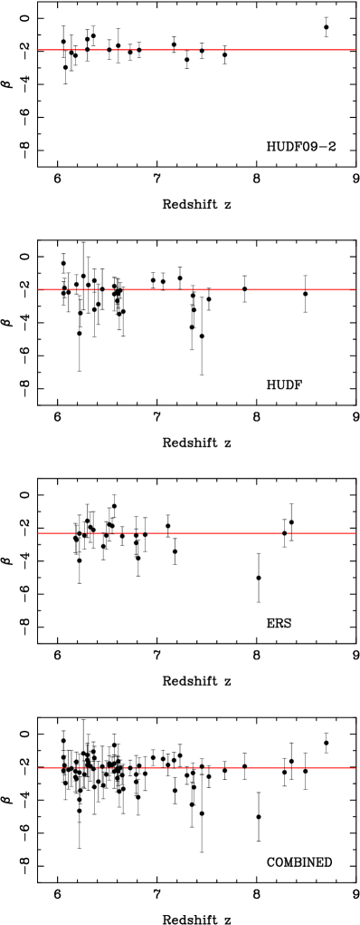
depending on the available filters and the redshift of the candidate. To derive the above formulae we have adopted the following pivot wavelengths for the $Y_{098},Y_{105},J_{125}$ & $H_{160}$ filters: 0.9864$\mu$m, 1.0552$\mu$m, 1.2486$\mu$m & 1.5369$\mu$m (WFC3 Instrument Handbook for Cycle 19). In order to sample as similar a range of rest-frame wavelengths as possible, and to ensure no potential contamination from Ly$\alpha$ line emission, the values of $\beta$ have been calculated using equations 2 or 3 for candidates at $z_{phot}\leq 6.4$ and equation 1 for those candidates at $z_{phot}>6.4$. In Fig. 4 we plot the estimated UV spectral slopes versus photometric redshift for the final robust sample, split by field. Several features of this plot are worthy of comment and are briefly discussed below.

4.1 Uncertainties on derived UV spectral slopes

As can readily be seen from Fig. 4, the uncertainties on measuring $\beta$ are typically large. This is simply a consequence of attempting to determine a spectral slope using two filters which are not well separated in wavelength. As an illustration, consider a galaxy at $z=7$ with a canonical UV spectral slope of $\beta=-2$, which is detected at $5\sigma$ significance in both the $J_{125}$ and $H_{160}$ filters. The corresponding estimate of the UV spectral slope is $\beta=-2.0\pm 1.3$, where the error simply reflects the photometric uncertainty. Clearly, deriving meaningful estimates of $\beta$ on an individual object-by-object basis requires significantly better than $5\sigma$ photometry in both filters. One obvious method of overcoming this problem is to assume that each $\beta$ measurement, although inaccurate, is at least unbiased. In which case, one can proceed to bin the data and attempt to estimate the mean value of $\beta$. However, even when adopting this approach, it is necessary to account for the wide range in $\beta$ uncertainties displayed by the objects in a typical sample, by calculating a properly weighted mean:

$$\langle\beta\rangle=\frac{\displaystyle\sum_{i=1}^{n}\frac{\beta_{i}}{\sigma_{i}^{2}}}{\displaystyle\sum_{i=1}^{n}\frac{1}{\sigma_{i}^{2}}}$$ (4)

where $\beta_{i}$ represents an individual $\beta$ measurement for a single candidate, and $\sigma_{i}^{2}$ is the corresponding variance.

4.2 Average values of UV spectral slopes

The variance-weighted values of $\langle\beta\rangle$ for each sub-sample, and the full combined sample are listed in Table 5 where, for comparison, we also list the straight arithmetic means and standard errors. It can be seen from Table 5 that for the HUDF and ERS sub-samples (and for the full combined sample), the variance-weighted mean results in a significantly redder estimate of the typical value of the UV slope than the straight arithmetic mean. Interestingly, for the HUDF09-2 sub-sample, where the photometry is most robust (see discussion below), the difference between the two estimates is negligible.

The results listed in Table 5 indicate that the ERS sub-sample contains a higher percentage of objects with $\beta\leq-2$ than the other two fields (based on the variance-weighted means), although the difference is not significant. However, it is worth noting that any suggestion that the ERS candidates display bluer UV spectral slopes cannot be due to a trend for increasingly blue UV spectral slopes with decreasing UV luminosity, given that the median absolute magnitude of the ERS sample is $M_{1500}=-20.2$ compared to $M_{1500}=-19.1$ for the HUDF. Overall, our results provide no evidence that the members of the $z\geq 6.5$ LBG population display values of $\beta$ significantly different from those seen in comparably luminous LBGs in the redshift interval $3<z<5$.

Table 5: Estimates of the typical value of the UV spectral slope ($\beta$) for our final robust sample. The first two columns list the names and sizes of the different samples being considered. Columns three and four list the variance-weighted and arithmetic mean values of $\beta$ respectively, together with their corresponding uncertainties. Note that candidate HUDF09-2$\_$2765 has been excluded from these calculations because it provides a biased estimate of $\beta$ due to its high redshift ($z_{phot}=8.7\pm 0.3$).

Sample	N	$\langle\beta_{\rm var}\rangle$	$\langle\beta_{\rm arith}\rangle$
HUDF	31	$-1.99\pm{0.14}$	$-2.40\pm{0.18}$
HUDF09-2	15	$-1.90\pm{0.15}$	$-1.91\pm{0.13}$
ERS	23	$-2.32\pm{0.18}$	$-2.52\pm{0.19}$
COMBINED	69	$-2.05\pm{0.09}$	$-2.33\pm{0.11}$

4.3 Potential for bias

It can be seen from Fig. 4 that the HUDF09-2 sub-sample seems to display a particularly tight distribution of UV slopes, whereas the HUDF and ERS sub-samples show considerably more scatter. At least part of the explanation for this is that the HUDF09-2 sub-sample has the most robust WFC3/IR photometry. The reason is that, although the WFC3/IR imaging of HUDF09-2 is deep (particularly the $J_{125}$ data), the supporting data at other wavelengths is not, in a relative sense, as good (e.g. no $B_{435}$ data, relatively shallow $V_{606}$+$i_{775}$ data, and no $4.5\mu$m data). As a consequence, candidates in the HUDF09-2 field are required to be somewhat brighter in the near-IR in order to pass our robustness criteria (see photometry in Appendix B).

Another noteworthy point is that the bluer mean UV slope in the ERS is probably connected to the relative depths of the WFC3/IR imaging in this field. Due to the fact that the $J_{125}$ imaging in the ERS is significantly deeper than the accompanying $Y_{098}$ and $H_{160}$ imaging, the ERS sub-sample is the closest of the three to being purely $J_{125}-$selected. It is clear that when estimating the UV spectral slope from the $J_{125}-H_{160}$ colour, selecting the sample largely on the apparent $J_{125}$ magnitude must introduce the potential for biasing the sample towards objects with blue values of $\beta$. A proper investigation of the sources of bias, and the potential for constraining the true underlying distribution of UV spectral slopes, requires detailed simulation work which, although beyond the scope of this paper, is investigated in detail by Dunlop et al. (2011).

Figure 5: Stellar mass versus absolute UV magnitude ($M_{1500}$) for the final robust sample of seventy $z\geq 6$ LBGs, where $M_{1500}$ is derived from the best-fitting SED models using a 100Å -wide filter centred on a rest-frame wavelength of 1500Å. In each panel, the small open circles are objects with non-detections (i.e. $\leq 2\sigma$) at 3.6$\mu$m, the large grey circles are objects which are detected at $3.6\mu$m and the large black circles are objects detected at both $3.6\mu$m and $4.5\mu$m. In the left-hand panel the stellar-mass measurements are based on our SED-fitting analysis using the full range of star-formation histories, metallicities and reddening described in Section 3.3. In the right-hand panel the stellar-mass measurements are based on a single set of SED templates with a constant star-formation rate, $Z=0.2Z_{\odot}$ and zero reddening (CSF model, see text for details). In the left-hand panel the thick black line is our best-fitting $M_{\star}-L_{\rm UV}$ relation (Equation 5) and the dotted line indicates the lower limit enforced by insisting that each candidate has an age $\geq 10$ Myrs. Those objects which lie on the lower limit (small grey open circles) have very poorly constraint stellar masses and were not included in the derivation of the best-fitting $M_{\star}-L_{\rm UV}$ relation. In both panels the thick grey line is the $M_{\star}-L_{\rm UV}$ relation (corrected to Chabrier IMF) derived by González et al. (2011) using a large sample of LBGs at $z\simeq 4$. In the right-hand panel the upper dotted line indicates the expected $M_{\star}-L_{\rm UV}$ relation for a CSF model which has been forming stars for $\simeq 600$ Myrs (i.e. since $z\simeq 20$ for an object at the mean redshift of the final robust sample; $z=6.8\pm 0.1$).

Table 6: The best-fitting parameters returned by our SED-fitting analysis of the twenty-one objects in our final robust sample with detections at either $3.6\mu$m or $3.6+4.5\mu$m. The first column lists the objects IDs. The second column lists the best-fitting star-formation history (SFH) which is either: an instantaneous burst (Burst), constant star-formation rate (Const) or exponentially decaying star-formation rate (E). For the those objects where the best-fitting SFH is exponentially decaying (i.e. SFR $\propto e^{(-t/\tau)}$), the proceeding number indicates the characteristic star-formation timescale in Gyrs (i.e. E0.2 $\Rightarrow\tau=0.2$ Gyrs). Columns 3-8 list the metallicity, age, reddening, stellar mass, star-formation rate and $\chi^{2}$ of the best-fitting SED template. For those objects where the best-fitting SFH is a Burst, the SFR listed in column 7 is derived from the best-fitting model with a constant or exponentially decaying SFH. Note that the ages listed in columns 4 & 10 refer to the total age of the system, rather than a luminosity-weighted age. Columns 9-12 list the $\chi^{2}$, age, stellar mass and SFR of the best-fitting constant SFR model with a metallicity of $0.2Z_{\odot}$ and $A_{\rm v}=0.0$ (CSF model, see text for details). Based on this restricted set of SED parameters those objects highlighted with a $\dagger$ symbol in column 9 would have been rejected because their best-fitting SED templates have an unacceptably high $\chi^{2}$. The final column lists an estimate of the SFR based on the UV luminosity of each object ($M_{1500}$), with no correction for dust attenuation, which has been derived using the Madau, Pozzetti & Dickinson (1998) formula (corrected to a Chabrier IMF).

ID	SFH	$Z$	Age	Av	$M_{\star}$00	SFR000	$\chi^{2}_{b}$	$\chi^{2}_{c}$	Age	$M_{\star}$	SFR	SFRUV
		($Z_{\odot}$)	(Myrs)		($10^{9}\hbox{$\rm\thinspace M_{\odot}$}$)	($\rm\thinspace M_{\odot}$yr-1)			(Myrs)	($10^{9}\hbox{$\rm\thinspace M_{\odot}$}$)	($\rm\thinspace M_{\odot}$yr-1)	($\rm\thinspace M_{\odot}$yr-1)
HUDF$\_1016$	Burst	$0.02$	010	1.1	00.9${}^{+0.3}_{-0.5}$	40.0${}^{+13.8}_{-11.3}$	4.3	19.3†	575	0.9${}^{+0.5}_{-0.4}$	2.1${}^{+0.1}_{-0.1}$	03.8
HUDF$\_522$	Burst	$0.02$	050	0.1	01.8${}^{+0.9}_{-1.0}$	15.0${}^{+6.8}_{-1.9}$	4.5	06.9	365	1.6${}^{+1.0}_{-0.4}$	6.4${}^{+0.3}_{-0.4}$	011.3
HUDF$\_658$	Burst	$0.50$	065	0.0	01.9${}^{+1.9}_{-1.0}$	02.5${}^{+3.3}_{-0.3}$	1.4	05.2	725	2.4${}^{+0.6}_{-0.9}$	5.1${}^{+0.1}_{-0.4}$	08.6
HUDF$\_860$	Burst	$0.50$	100	0.1	02.6${}^{+2.6}_{-0.5}$	01.8${}^{+2.0}_{-0.1}$	1.8	17.8†	645	1.5${}^{+0.4}_{-0.5}$	3.4${}^{+0.3}_{-0.3}$	05.4
HUDF$\_1173$	Burst	$0.02$	055	0.0	00.6${}^{+1.4}_{-0.5}$	01.1${}^{+2.1}_{-0.4}$	4.5	04.7	455	0.8${}^{+0.8}_{-0.5}$	2.4${}^{+0.5}_{-0.3}$	04.5
HUDF09-2$\_1543$	Const	$0.02$	725	0.1	02.1${}^{+3.1}_{-1.3}$	04.5${}^{+1.3}_{-2.6}$	0.3	00.4	575	1.5${}^{+0.9}_{-0.3}$	4.0${}^{+0.4}_{-0.4}$	07.8
HUDF09-2$\_2587$	Const	$0.02$	645	0.6	06.3${}^{+3.6}_{-3.4}$	13.8${}^{+4.4}_{-7.6}$	3.3	09.5†	815	2.3${}^{+0.6}_{-0.9}$	4.1${}^{+0.1}_{-0.3}$	07.2
HUDF09-2$\_1660$	E1.0	$0.02$	725	0.5	06.9${}^{+1.8}_{-5.1}$	010.0${}^{+2.8}_{-6.1}$	3.8	08.7†	815	2.1${}^{+1.3}_{-0.5}$	4.1${}^{+0.3}_{-0.3}$	07.2
HUDF09-2$\_1584$	E0.2	$0.20$	725	0.1	16.5${}^{+9.6}_{-13.3}$	03.8${}^{+0.5}_{-3.6}$	0.7	07.6†	645	2.3${}^{+0.6}_{-0.9}$	5.3${}^{+0.3}_{-0.3}$	09.4
ERS$\_7086$	Burst	$0.02$	025	0.1	00.4${}^{+0.4}_{-0.1}$	0 4.9${}^{+4.1}_{-2.6}$	1.4	01.7	130	0.4${}^{+0.4}_{-0.6}$	3.6${}^{+2.3}_{-0.5}$	06.5
ERS$\_6066$	E0.2	$1.00$	645	0.1	13.4${}^{+3.5}_{-8.0}$	04.4${}^{+0.4}_{-0.5}$	2.7	25.4†	815	2.4${}^{+0.6}_{-0.9}$	4.4${}^{+0.4}_{-0.3}$	07.2
ERS$\_9100$	E0.2	$0.50$	405	0.0	01.8${}^{+2.6}_{-0.9}$	02.0${}^{+1.3}_{-0.8}$	1.4	03.2	815	1.4${}^{+0.4}_{-0.5}$	2.6${}^{+0.3}_{-0.4}$	04.5
ERS$\_7225$	E0.05	$0.20$	325	0.0	06.4${}^{+6.4}_{-1.3}$	00.4${}^{+1.9}_{-0.1}$	4.3	28.0†	815	1.9${}^{+0.5}_{-0.8}$	3.6${}^{+0.4}_{-0.4}$	06.0
ERS$\_6438$	Burst	$0.20$	160	0.0	04.5${}^{+2.6}_{-2.3}$	03.6${}^{+0.4}_{-0.4}$	6.7	14.9†	725	2.1${}^{+0.5}_{-0.8}$	4.5${}^{+0.3}_{-0.5}$	07.2
ERS$\_6263$	Burst	$0.02$	330	0.0	00.5${}^{+1.1}_{-0.4}$	02.5${}^{+5.3}_{-0.8}$	4.9	05.3	130	0.4${}^{+0.6}_{-0.3}$	4.3${}^{+4.4}_{-0.8}$	07.2
ERS$\_7776$	E0.2	$0.02$	325	0.0	01.1${}^{+1.1}_{-0.8}$	02.1${}^{+1.1}_{-1.3}$	3.9	04.2	515	1.0${}^{+0.6}_{-0.6}$	2.9${}^{+0.5}_{-0.4}$	05.4
ERS$\_5847$	E1.0	$0.20$	815	0.0	03.3${}^{+4.9}_{-2.4}$	04.1${}^{+1.1}_{-2.8}$	2.7	02.9	815	2.4${}^{+2.4}_{-1.4}$	4.4${}^{+0.4}_{-0.4}$	08.6
ERS$\_3679$	Burst	$0.02$	725	0.2	04.5${}^{+6.8}_{-2.6}$	15.0${}^{+0.9}_{-10.6}$	5.5	08.3	725	4.3${}^{+1.1}_{-1.5}$	8.9${}^{+0.3}_{-0.8}$	16.4
ERS$\_7412$	Burst	$1.00$	010	0.2	00.4${}^{+0.8}_{-0.3}$	011.4${}^{+7.1}_{-2.9}$	9.1	12.2†	255	0.8${}^{+0.8}_{-0.5}$	3.9${}^{+1.1}_{-0.5}$	06.5
ERS$\_6427$	E0.2	$0.02$	575	0.0	04.4${}^{+4.4}_{-1.6}$	02.1${}^{+0.4}_{-0.8}$	1.2	06.6	725	2.0${}^{+0.5}_{-0.4}$	4.1${}^{+0.4}_{-0.5}$	07.2
ERS$\_7376$	Const	$0.20$	455	0.0	01.1${}^{+1.6}_{-0.9}$	03.5${}^{+1.1}_{-2.5}$	0.6	00.6	455	1.1${}^{+1.1}_{-0.8}$	3.5${}^{+0.9}_{-0.5}$	06.5

5 Stellar masses and star-formation rates

A key advantage of employing a template-fitting SED analysis is that stellar mass and star-formation rate estimates can be directly derived from the best-fitting models. In this Section we use this information to investigate the relationship between stellar mass and UV luminosity, and try to determine the typical specific star-formation rate (sSFR) for $L^{\star}$ LBGs at $z\geq 6$. Throughout this Section we will repeatedly refer to the results for a sub-sample of twenty-one objects which have the most reliable star-formation rate and stellar-mass estimates because they are detected at either 3.6$\mu$m or $3.6+4.5\mu$m. In Table 6 we list the best-fitting parameters returned by our SED-fitting analysis for these objects, based on the best-fitting templates drawn from the full range of star-formation histories, metallicities and reddening described in Section 3.3. Based on photometry alone it is very difficult to accurately constrain the star-formation history and metallicity of high-redshift galaxies. As a result, it is common in the literature to derive star-formation rate and stellar-mass estimates from a much more restricted set of SED templates (typically constant star-formation rate models). In order to investigate the effect of this approach, in Table 6 we also list the best-fitting parameters derived from an SED template with a constant star-formation rate, $Z=0.2Z_{\odot}$ and zero reddening (CSF model).

5.1 Stellar mass - UV luminosity relation

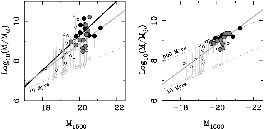
In Fig. 5 we plot stellar mass versus absolute UV magnitude ($M_{1500}$) for our final robust sample of seventy $z\geq 6$ LBGs. In the left-hand panel we plot stellar-mass estimates based on the best-fitting SED templates drawn from the full grid of star-formation histories, metallicities and reddening. In the right-hand panel we plot the stellar-mass estimates based on the CSF model alone. In both panels the small open circles indicate those objects which are formally undetected at $3.6\mu$m. For these objects the only stellar mass constraints at $\lambda_{\rm{rest}}\geq 4000$Å  come from the upper limits at $3.6/4.5\mu$m provided by the deconfusion analysis. In contrast, those objects which are detected at $3.6\mu$m ($\geq 2\sigma$) are plotted as large grey circles, and those objects detected at both $3.6\mu$m and $4.5\mu$m are plotted as large black circles.

Based on the data presented in left-hand panel of Fig. 5 we have used the fitxy routine (Press et al. 1992) to derive the following relationship between stellar mass and UV luminosity ($L_{1500}$):

$$\log\left(\frac{M_{\star}}{\hbox{$\rm\thinspace M_{\odot}$}}\right)=(2.14\pm 0.56)\log\left(\frac{L_{1500}}{{\scriptstyle{\rm WHz}}^{-1}}\right)-37.05\pm 4.52$$ (5)

which is shown as the thick black line in the left-hand panel of Fig. 5. It is interesting to compare our equation 5 with the $M_{\star}~{}-~{}L_{\rm UV}$ relation derived by González et al. (2011) based on $\simeq 500$ $B-$drop galaxies at $z\simeq 4$. The $M_{\star}-L_{\rm UV}$ relation derived by González et al. (2011) is plotted as the thick grey line in both panels of Fig. 5, and has the form: $M_{\star}\propto L_{1500}^{1.7\pm 0.2}$. It can be seen from the left-hand panel of Fig. 5 that both relations are clearly consistent, although the $M_{\star}-L_{\rm UV}$ relation derived here for LBGs with a mean redshift of $z=6.8\pm 0.1$ is somewhat steeper.

In an earlier study, Stark et al. (2009) also explored the $M_{\star}~{}-~{}L_{\rm UV}$ relation based on $4<z<6$ LBGs selected from the GOODS N+S fields. At $z\simeq 4$ the data from Stark et al. (2009), based on a sample of $\simeq 700$ $B-$drop candidates, is entirely consistent with the $M_{\star}-L_{\rm UV}$ relation derived by González et al. (2011). At higher redshifts, both Stark et al. (2009) and González et al. (2011) investigated the $M_{\star}-L_{\rm UV}$ relation at $z\simeq 5$ and $z\simeq 6$, based on samples of $V-$drop and $i-$drop LBG candidates respectively. Interestingly, at $z\simeq 5$ the results of both studies do appear to be consistent with a steepening of the $M_{\star}-L_{\rm UV}$ relation. In fact, this effect was noted by Stark et al. (2009) but, based on the available data, both authors concluded that there was no strong evidence for redshift evolution. At $z\simeq 6$ neither study had sufficient dynamic range in $L_{\rm UV}$ to constrain the slope of the $M_{\star}-L_{\rm UV}$ relation.

At a given UV luminosity, the range of stellar masses displayed by the LBG candidates in Fig. 5 is simply a function of their $M_{\star}/L_{\rm UV}$ ratios which, in turn, are largely a function of their stellar population ages. Unfortunately, those candidates which have neither detections or meaningful upper limits at IRAC wavelengths inevitably have stellar ages/masses which are very poorly constrained (small grey open circles in Fig. 5). These objects (which we have excluded from our determination of the best-fitting $M_{\star}-L_{\rm UV}$ relation) can be seen to congregate close to the lower limit which is imposed during the SED-fitting procedure by insisting that each candidate must have an age of $\geq 10$ Myr. However, in reality, the majority of these objects can tolerate SED fits with stellar populations as old as $\simeq$ 200 Myrs, at which point their estimated stellar masses become an order of magnitude larger. Consequently, the apparent steepening of the $M_{\star}-L_{\rm UV}$ relation at faint magnitudes must be viewed with considerable caution.

It is clear from Fig. 5 that, based on the current sample, it is not possible to determine if the $M_{\star}-L_{\rm UV}$ relation at $z\geq 6$ is steeper than at $z\simeq 4$. Indeed, our results for the twenty-one objects with the most reliable stellar-mass estimates are entirely consistent with the conclusion that the slope and normalisation of the $M_{\star}-L_{\rm UV}$ relation does not change over the redshift interval $4.0<z<7.0$. However, by restricting ourselves to those objects with the most reliable stellar-mass estimates, the results presented in the left-hand panel of Fig. 5 suggest that $L^{\star}$ ($M_{1500}\simeq-20.2$) galaxies at $z\simeq 6.5$ have a median stellar mass of $M_{\star}~{}=~{}(2.1\pm~{}1.1)\times 10^{9}\hbox{$\rm\thinspace M_{\odot}$}$. Moreover, by deriving stellar-mass estimates using stellar population models covering a wide range of metallicities, star-formation histories and reddening, our results indicate that the full range of $M_{\star}/L_{\rm UV}$ ratios displayed by $L^{\star}$ galaxies at this epoch could span a factor of $\simeq 50$.

Within this context it is interesting to compare the left-hand and right-hand panels of Fig. 5 where the limiting effect of restricting the SED-fitting to a constant star-formation rate (CSF) model is explored. It can immediately be seen from the right-hand panel that if we adopt the same approach as González et al. (2011) and restrict our SED-fitting to the CSF model, our stellar-mass estimates at $z\simeq 6.8$ fall into excellent agreement with the $M_{\star}-L_{\rm UV}$ relation they derived at $z\simeq 4$. Moreover, it is also clear that restricting the SED-fitting analysis to the CSF model significantly reduces (perhaps unrealistically) the scatter in the stellar-mass estimates at a given UV luminosity. Finally, as illustrated by the upper dotted line in the right-hand panel of Fig. 5, the brightest LBGs in our sample (i.e. $M_{1500}\leq 19.0$) are fully consistent with the expected $M_{\star}-L_{\rm UV}$ relation for a galaxy which has been forming stars at a constant rate for $\simeq 600$ Myrs. Importantly, at the mean redshift of the final robust sample ($z=6.8\pm 0.1$), 600 Myrs represents $\simeq 80\%$ of the age of the Universe. Indeed, the primary cause of the clustering of objects around the $M_{\star}-L_{\rm UV}$ relation corresponding to $\simeq 600$ Myrs of constant star-formation is the requirement imposed during the SED-fitting that objects must be younger than the age of the Universe. The underlying cause is simply that (with no dust reddening) the CSF models are bluer than the observed photometry unless their age is close to the maximum allowable at this epoch. In summary, although the results shown in both panels of Fig. 5 are broadly compatible, it is clear that adopting a restricted set of SED templates may well provide a misleadingly low estimate of the true level of scatter in stellar mass at a given UV luminosity.

Before moving on to consider the relationship between stellar mass and star-formation rate, it is worth remembering that one of the principal motivations for studying the $M_{\star}-L_{\rm UV}$ relation at high redshift is to constrain the galaxy stellar-mass function (e.g. McLure et al. 2009). The results presented in Fig. 5 clearly illustrate that in order to successfully constrain the stellar-mass function at $z\geq 6.5$ is will be necessary to constrain the $M_{\star}-L_{\rm UV}$ relation at UV luminosities substantially fainter than $L^{\star}$. Over the next three years, the new Cosmic Assembly Near-infrared Deep Extragalactic Legacy Survey (CANDELS; Co-P.I.s S. Faber & H. Ferguson; see Grogin et al. 2011 and Koekemoer et al. 2011) offers the prospect of significant progress. The deep portion of CANDELS will provide $Y_{105},J_{125}\,\&\,H_{160}$ WFC3/IR imaging to $m_{AB}\simeq 28(5\sigma)$ over an area of $\simeq 150$ sq. arcmins in the GOODS N+S fields. The CANDELS programme should therefore provide a sample of $\mbox{{\raisebox{-1.72218pt}{$\stackrel{{\scriptstyle>}}{{{\scriptstyle\sim}}}$}}}\,200$ robust $z\simeq 7$ candidates in the magnitude range $-19>M_{1500}>-20$, all covered by the deep IRAC imaging available in GOODS N+S. A sample of this size should be sufficient to obtain robust constraints on the typical $M_{\star}/L_{\rm UV}$ ratio at $M_{1500}\simeq-19$ by employing a stacking analysis to provide the necessary IRAC photometry. Obtaining constraints on the $M_{\star}-L_{\rm UV}$ relation at magnitudes as faint as $M_{1500}\simeq-18.5$ (i.e. $\simeq 0.2L^{\star}$ at $z\simeq 7$) will rely on stacking the final epoch2 WFC3/IR imaging of the HUDF into the forthcoming, ultra-deep, IRAC data being obtained as part of the Cycle 7 Spitzer warm mission GO-70145 (P.I. Labbé).

Figure 6: Star-formation rate versus stellar mass for the twenty-one objects in our final robust sample with IRAC detections at either 3.6$\mu$m (grey) or 3.6+4.5$\mu$m (black). In the left-hand panel the star-formation rates and stellar masses have been measured from the best-fitting SED template drawn from the full range of star-formation histories, metallicities and reddening described in Section 3.3. In the right-hand panel the star-formation rates and stellar masses have been estimated from the best-fitting CSF model (see text for details). The $1\sigma$ errors on both parameters have been calculated by determining the $\Delta\chi^{2}=1$ interval, after marginalization over all other free parameters. The solid line in both panels is the SFR$-M_{\star}$ relation derived by Daddi et al. (2007) for star-forming galaxies at $z\simeq 2$ and corresponds to a sSFR of $\simeq 2.5$ Gyr^-1. In the right-hand panel the dotted lines illustrate how the SFR$-M_{\star}$ relation for a galaxy with a constant star-formation rate and zero reddening varies as a function of stellar population age.

5.2 Star-formation rate versus stellar mass

Over recent years it has become clear that studying the ratio of the current star-formation rate to the previously assembled stellar mass (SFR/$M_{\star}$), the so-called specific star-formation rate (sSFR), can provide a useful insight into the average star-formation history of a galaxy population. Studies of star-forming galaxies in the SDSS at $z\simeq 0.1$ (Brinchmann et al. 2004), in the Extended Groth Strip at $z\simeq 1.0$ (Noeske et al. 2007) and in the GOODS fields at $z\simeq 1.0$ and $z\simeq 2.0$ (Elbaz et al. 2007; Daddi et al. 2007) have consistently shown a correlation of the form SFR $\propto$ $M_{\star}^{0.9}$ (sSFR $\propto M_{\star}^{-0.1}$), over a wide dynamic range in stellar mass. Moreover, these studies have shown that compared to a median value of sSFR $\simeq 2.5$ Gyr^-1 at $z=2$ (Daddi et al. 2007), the normalisation of the sSFR$-M_{\star}$ relation has decreased by a factor of $\simeq 40$ over the last 10 Gyrs.

Indeed, there is some evidence that a sSFR of $\simeq 2.5$ Gyr^-1 may represent the maximum sustainable star-formation rate for galaxies at $z\geq 2$. A recent study by Karim et al. (2011) found that high mass ($M_{\star}\geq 10^{10}\hbox{$\rm\thinspace M_{\odot}$}$) star-forming galaxies in the COSMOS field consistently follow a steeper sSFR-$M_{\star}$ relation than determined by previous studies (sSFR $\propto M_{\star}^{-0.4}$). However, by $z\simeq 3$ the results of Karim et al. (2011) suggest that the sSFR-$M_{\star}$ relation flattens at masses of $M_{\star}\leq 10\hbox{$\rm\thinspace M_{\odot}$}$, becoming consistent with sSFR $\propto M_{\star}^{-0.1}$. Karim et al. (2011) interpret this flattening as a result of a natural limit to the sustainable sSFR of $\simeq 2.5$ Gyr^-1, corresponding roughly to the inverse of the typical galaxy free-fall timescale. Within this context, it is interesting to note that González et al. (2010) recently found that the median sSFR of a sample of twelve $z-$drop candidates at $z\simeq 7$ was also $\simeq 2.5$ Gyr^-1.

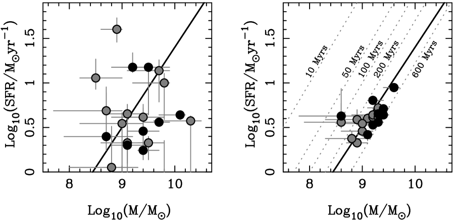
In Fig. 6 we plot SFR versus stellar mass for the twenty-one objects which have IRAC detections and therefore the most robust SFR and stellar-mass estimates. In the left-hand panel the stellar mass and dust corrected SFR estimates have been taken from the best-fitting SED templates drawn from the full range of star-formation histories, metallicities and dust reddening described in Section 3.3. In contrast, in the right-hand panel the stellar mass and SFR estimates have been taken from the best-fitting CSF model. Although the distribution of objects in the two panels is significantly different, both provide a consistent estimate for the typical sSFR. In the left-hand panel the median sSFR is $1.9\pm 0.8$ Gyr^-1, while in the right-hand panel the median sSFR is $2.6\pm 0.4$ Gyr^-1. Both estimates are clearly consistent with the typical sSFR value for $z\simeq 2$ star-forming galaxies estimated by Daddi et al. (2007). To illustrate this point, in both panels of Fig. 6 the thick solid line is the best-fitting SFR-$M_{\star}$ relation from Daddi et al. (2007) which corresponds to a sSFR of $\simeq 2.5$ Gyr^-1.

Consequently, taken at face value, our results provide additional support to the conclusion that a direct proportionality between SFR and stellar mass is still viable at $z\simeq 6.5$, and that the corresponding sSFR of $\simeq 2.5$ Gyr^-1 may correspond to a physical limit on the maximum sustainable star-formation rate. However, it is clear from the left-hand panel that allowing a reasonable range of star-formation histories, metallicities and dust reddening leads to a large scatter in the SFR at a given stellar mass. Consequently, although the data shown in the left-hand panel are consistent with SFR and stellar mass being roughly proportional, they are also entirely consistent with star-formation and stellar mass being entirely unrelated. In contrast, the results shown in the right-hand panel suggest that SFR and stellar mass are well correlated, lying along a SFR$-M_{\star}$ relation with a slope close to unity and a normalization consistent with a sSFR of $\simeq 2.5$ Gyr^-1.

However, it is worth noting that the apparently simple picture presented in the right-hand panel of Fig. 6 probably reflects limitations of relying on the CSF model, rather than offering genuine physical insight into high-redshift star-formation. The simple reason for this caution is that the agreement is largely inevitable when you only consider SEDs with constant star-formation and no reddening. In this situation, each object is required to lie on a relation with slope of unity, with it’s position on the SFR$-M_{\star}$ plane simply determined by the best-fitting age. To illustrate this point we have plotted the expected SFR$-M_{\star}$ relations for CSF models of various stellar population ages as the dotted lines in the right-hand panel of Fig. 6. This demonstrates that, provided the typical stellar population age lies in the range 200-600 Myrs, the resulting SFR$-M_{\star}$ relation will automatically have a slope close to unity, and result in a typical sSFR consistent with $\simeq 2.5$ Gyr^-1.

In summary, although it is possible to constrain the typical sSFR of $L^{\star}$ LBGs at $z\simeq 6.5$, the limitations of the current sample do not allow meaningful constraints to be placed on the form of the SFR$-M_{\star}$ relation. In order to resolve this issue it will be necessary to obtain much larger samples of $z\geq 6$ LBGs with stellar masses $M_{\star}\geq 10^{8.5}\hbox{$\rm\thinspace M_{\odot}$}$. Within this context, the new CANDELS WFC3/IR imaging data should prove decisive. The wide portion of CANDELS will proved $J_{125}+H_{160}$ imaging to a depth of $m_{AB}\simeq 27(5\sigma)$ over an area of $\simeq 0.2$ sq. degrees, all of which is covered by deep IRAC imaging at $3.6+4.5\mu$m ($m_{AB}\simeq 26$, $5\sigma$) provided by the Spitzer Extended Deep Survey (SEDS; P.I. G. Fazio). The combination of CANDELS+SEDS should therefore allow the SFR$-M_{\star}$ relation at $z\simeq 6.5$ to be investigated using a sample of $\mbox{{\raisebox{-1.72218pt}{$\stackrel{{\scriptstyle>}}{{{\scriptstyle\sim}}}$}}}\,250$ LBGs with reliable stellar-mass estimates of $M_{\star}\geq 10^{8.5}\hbox{$\rm\thinspace M_{\odot}$}$.

5.3 The effect of nebular emission

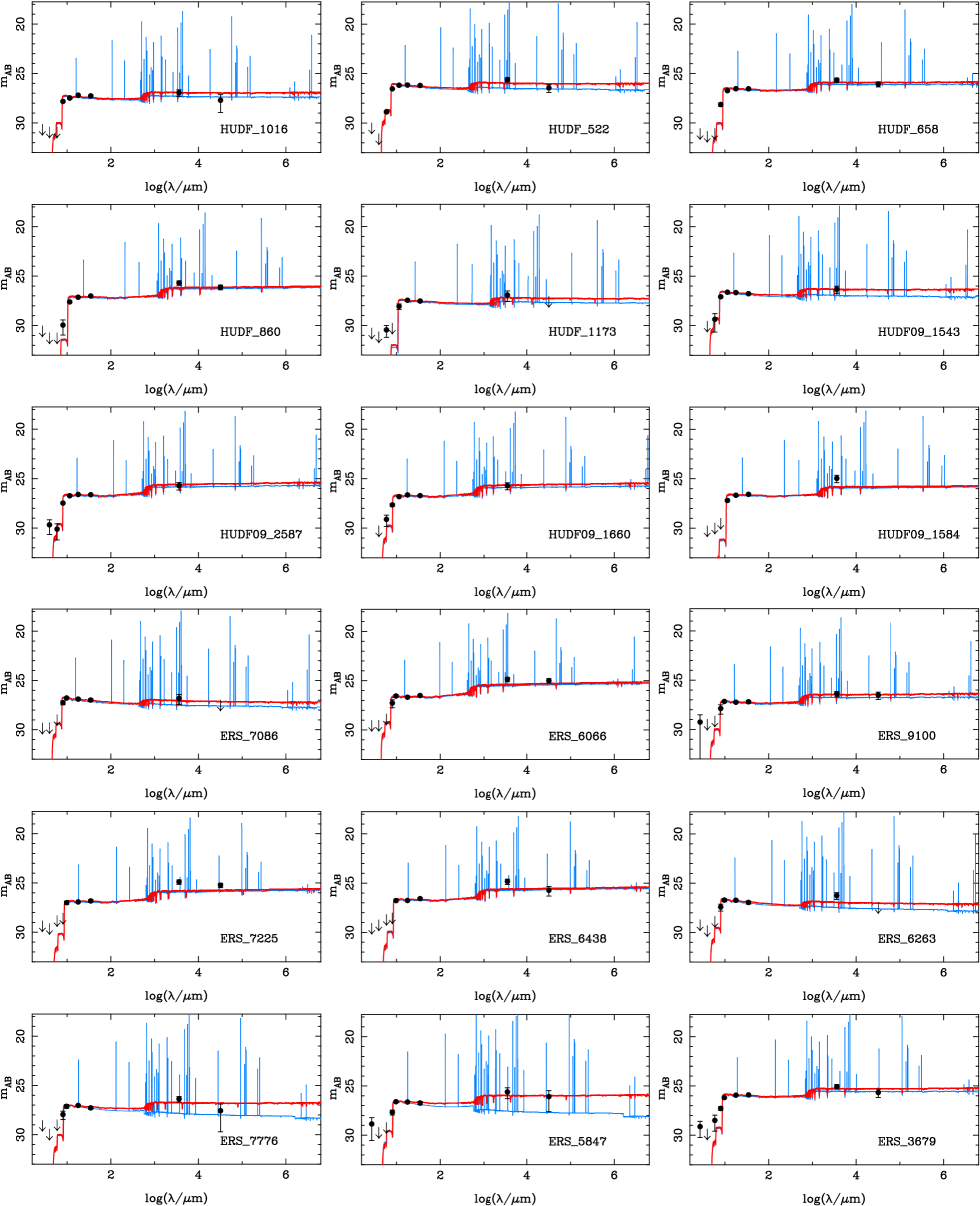
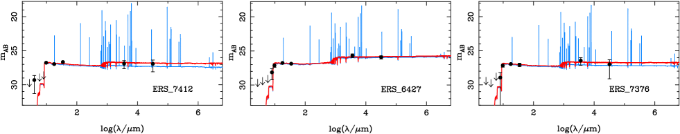
Recent work has suggested that nebular continuum and line emission might contribute to the observed SEDs of $z\sim 6-7$ galaxies (e.g. Ono et al. 2010; Schaerer et al. 2010). As discussed by Robertson et al. (2010), galaxies with strong UV continua can typically be fit using pure stellar populations with ages of a few hundred Myr, or by much younger populations ($\leq$ few Myr) with significant nebular contributions and an implied low escape fraction ($f_{\mathrm{esc}}$) of Lyman continuum photons. Such nebular solutions can yield much lower stellar masses than those in the purely stellar case (Ono et al. 2010).

In order to quantify this degeneracy and its possible effect on our derived physical properties, we have examined in more detail the sub-sample of twenty one galaxies detected in the 3.6 $\mu$m IRAC band (nine of which are also detected at 4.5$\mu$m). For these objects it is possible to investigate whether the IRAC detections can provide a valuable discriminant between the nebular and stellar solutions, given the location of prominent nebular lines, such as H$\beta$ and [OIII] 5007Å, at the redshifts of interest.

Figure 7: An example of our SED-fitting procedure using models which incorporate nebular continuum and line emission. In this illustration the pure stellar continuum model ($f_{\mathrm{esc}}=1$) is shown as the red (thick) line and the template featuring nebular emission ($f_{\mathrm{esc}}=0.2$) is shown as the blue (thin) line. For clarity the galaxy template featuring nebular emission has been displaced by 0.1 magnitudes (both models have a metallicity of Z = 0.2 Z_⊙).

5.3.1 Nebular emission methodology

As before we use the Bruzual & Charlot (2003) models to generate a set of spectral templates based on a Chabrier IMF. For the models presented here, we use a representative exponentially decaying star-formation history ($\tau\simeq 0.4$ Gyr) and, motivated by the fact that high-redshift galaxies often exhibit low metallicities (e.g. Finkelstein et al. 2011), we consider both solar (Z = Z_⊙) and fifth solar models (Z = 0.2 Z_⊙). In addition to exponentially decaying star-formation histories, we also investigated models with constant star formation, but found that these did not significantly alter our results. The contribution of the nebular continuum and line emission is computed in the manner of Robertson et al. (2010), providing nebular emission models similar to those calculated by Ono et al. (2010). The strength of the nebular emission is tied to the number of ionizing photons per second ($N_{\mathrm{Lyc}}$), calculated from the stellar population model, via the H$\beta$ luminosity (in erg s^-1):

$$L(H\beta)=4.78\times 10^{-13}(1-f_{\mathrm{esc}})N_{lyc}$$ (6)

Other HI line intensities follow from ratios predicted by standard recombination theory (Osterbrock & Ferland 2006). Lines from common metallic species are included using relative intensities given by Anders et al. (2003) assuming the gas phase metallicity is either Z_⊙ or 0.2 Z_⊙. We use the method of Brown et al. (1970) to calculate the strength of bound-free and free-free continuum emission, and use results from Osterbrock & Ferland (2006) for the two photon emission from H.

When fitting the SED models we consider two fixed values of the escape fraction, $f_{\mathrm{esc}}=0.2$ (stellar and nebular emission) and $f_{\mathrm{esc}}=1$ (purely stellar emission). The value of $f_{\mathrm{esc}}=0.2$ is motivated by direct observations of the Lyman continuum in galaxies at $z\sim 3$ (Shapley et al. 2006) and typical values of $f_{\mathrm{esc}}$ required for star-forming galaxies to maintain reionization at $z\sim 7$ (Robertson et al. 2010). As we are primarily interested in how nebular emission might alter the inferred stellar mass and age, we do not include the possible effects of Ly$\alpha$ emission or reddening. An example SED fit featuring nebular emission is shown in Fig. 7 and the 0.2 Z_⊙ nebular SED fits for all twenty one objects can be found in Appendix B.

Figure 8: A histogram of the ratio of the best-fitting stellar masses returned by fitting Z = 0.2 Z_⊙ SED models with ($M^{n}$) and without ($M^{\star}$) nebular continuum and line emission for the twenty one objects with $3.6\mu$m IRAC detections. For 16 out of 21 objects the stellar-mass estimates differ by less than a factor of 2.5. However, it can be seen that there are two objects for which the nebular fits return stellar masses which are an order of magnitude smaller than the stellar masses returned by fits without nebular emission.

5.3.2 Nebular emission results

For the models with sub-solar metallicity it is found that, compared to the purely stellar templates ($f_{\mathrm{esc}}=1$), the templates which include nebular emission ($f_{\mathrm{esc}}=0.2$) provide a better fit to 14 of the 21 objects, and all nine of the objects with detections in both IRAC bands. The data favour the nebular emission models because of the predominantly blue [3.6] - [4.5] $\mu$m observed colours that are easily reproduced by including rest-frame optical line emission. In contrast, the shape of the purely stellar model SEDs redward of the Balmer/$4000$Å  break cannot easily accommodate these blue rest-frame optical colours.

For the majority of this sub-sample (16 out of 21) the best-fitting ages are still $\geq$ 100 Myr with stellar masses reduced by less than a factor of 2.5 (see Fig. 8). In contrast, the best-fitting models to the remaining five galaxies have significantly lower stellar masses (by more than a factor of ten in two cases). Interestingly, all five of these objects are only detected in the 3.6 $\mu$m band and have best-fitting ages which are perhaps unphysical (median age 9 Myrs). Using solar metallicities, we find eight galaxies with significantly altered parameters, including all five found for models with Z = 0.2 Z_⊙.

In summary, with the current precision of the HST and IRAC photometry, we are unable to draw firm conclusions about the possible presence of nebular emission in these sources. However, given that the inferred stellar masses from the models including nebular emission are generally similar to those inferred from purely stellar models, we conclude that the results presented in Sections 5.1 and 5.2 appear to be robust to the inclusion of $f_{\mathrm{esc}}=0.2$ nebular emission, especially for those objects with detection in both IRAC bands.

6 Comparison with previous studies

As discussed in the introduction, the availability of the various new WFC3/IR datasets has led to a proliferation of papers focused on $z\geq 6$ LBGs. With authors each applying their individual candidate selection procedures, and in many cases using their own independent reductions of the publicly available data, it is difficult to obtain a clear overview of the subject, and to identify whether different studies are in good agreement, or not. Consequently, in this section we compare our final robust sample with those derived elsewhere in the literature (on a field-by-field basis), highlighting the objects we have in common, and investigating the properties of previously published high-redshift candidates which are not included in our final robust sample.

Given that one of the primary motivations for this study was to derive a sample of high-redshift candidates which is as robust as possible, and that previous samples of WFC3/IR high-redshift candidates were selected for a variety of purposes, it is not the case that we regard any object not included in our final sample as a low-redshift interloper. In fact, as the proceeding discussion will demonstrate, each of the candidates from the literature samples falls into one of four categories. The first category consists of objects which are in common with our final sample of seventy $z\geq 6$ LBGs and we therefore regard as being robust. The second category consists of objects which were not included in our final sample (because they failed to meet one or more of our adopted criteria), but which nevertheless our analysis suggests are likely to be at high redshift. The third category consists of objects which our analysis suggests are likely to be a low redshift, but do have an acceptable (albeit lower probability) solution at high redshift. The fourth category consists of those objects which our analysis suggests are very unlikely to be at high redshift. Throughout the discussion in this Section we have attempted to make it as clear as possible which category each of the candidates falls into. Finally, it should be noted that where a research group has published a number of studies of a particular survey field, we only discuss the results from the most recent study, under the assumption that they supersede any previous work.

6.1 HUDF

6.1.1 McLure et al. 2010

In McLure et al. (2010) we published our initial analysis of the HUDF WFC3/IR dataset, providing a list of N=49 high-redshift candidates with $z_{phot}\geq 5.9$. The candidate selection procedure employed in McLure et al. (2010) was broadly similar to that adopted here, with the most noteworthy difference between the two analyses being that in this work we have directly employed deconfused IRAC photometry in the candidate selection procedure.

Of the N=31 objects identified in the final HUDF sample listed in Table 2, N=28 are in common with the sample derived in McLure et al. (2010), demonstrating an excellent level of agreement between the two studies. However, there are N=21 candidates published in McLure et al. (2010) which do not feature in the final robust sample derived here. The reason behind this is that primary aim of McLure et al. (2010) was to provide an estimate of the $z=7$ and $z=8$ galaxy luminosity functions. Consequently, the McLure et al. (2010) sample was designed to be as complete as possible, and therefore contained all potential $z\geq 5.9$ LBGs revealed by the SED-fitting analysis, irrespective of whether or not they also displayed an acceptable low-redshift solution . In contrast, the principal aim of this study is to derive a sample of $z\geq 6$ LBG candidates which is as robust as possible, which means, in effect, requiring that any alternative low-redshift solutions can be statistically excluded. Although all N=21 of the additional candidates listed in McLure et al. (2010) also feature in the initial catalogues derived here, all of them were excluded from our final robust HUDF sample because the best-fitting alternative solutions at low-redshift could not be excluded at the $\Delta\chi^{2}\geq 4$ ($95\%$) level.

6.1.2 Bouwens et al. 2011

Based on their analysis of the HUDF dataset, Bouwens et al. (2011) list a total of N=31 robust high-redshift candidates, which are a mixture of $z-$drops and $Y-$drops. Of these N=31 candidates, eighteen also featured in our final robust sample of HUDF candidates listed in Table 2. However, it is clearly of interest to investigate why the remaining thirteen objects identified by Bouwens et al. (2011) do not feature in our final robust sample.

Firstly, we should note that six of the thirteen additional objects (UDFz-38537518, UDFy-37588003, UDFy-33446598, UDFy-39347255, UDFy-40338026 & UDFy-42406550) are simply too faint to make it into our final robust sample. None of these six objects is bright enough (in a 0.6^′′diameter aperture) to provide a $\geq 5\sigma$ detection in any of the WFC3/IR bands, and all six are fainter than any of our robust HUDF candidates. Consequently, this leaves a total of seven high-redshift candidates listed by Bouwens et al. (2011) which could, in principle, also feature in our final robust sample.

Our SED-fitting analysis suggests that two of the additional objects (UDFz-44746449 & UDFy-43086276) are likely to be at high-redshift ($z_{phot}=8.1$ and $z_{phot}=8.3$ respectively), but just failed to make our final robust sample because the competing low-redshift solutions could not be ruled-out at $\geq 95\%$ confidence. A further two additional objects (UDFz-42567314 & UDFz-42247087) also have primary photometric redshift solutions at $z_{phot}\geq 6.0$, but were subsequently rejected because they were either too close to the WFC3/IR array edge (UDFz-42567314), or were deemed to have unreliable photometry due to contamination from a nearby, bright, low-redshift galaxy (UDFz-42247087). Of the remaining three objects, one (UDFy-37796001) does have an acceptable solution at $z_{phot}\geq 8$, but was rejected because our analysis suggests that the alternative solution at $z_{phot}\simeq 2$ is marginally preferred. The other two (UDFz-37296175 & UDFy-37636015) were rejected because our SED fitting analysis returned a primary photometric redshift solutions at $z_{phot}\simeq 5$.

Finally, it can be seen from Table 2 that our final robust sample contains thirteen objects which are not featured in the Bouwens et al. (2011) robust candidate list. However, the noteworthy feature of these objects is that the vast majority (11/13) are at $z_{phot}\leq 6.5$, whereas the Bouwens et al., colour-colour, selection criteria are tuned to select objects at $z_{phot}\geq 6.5$. The two exceptions (HUDF$\_1730$ & HUDF$\_2701$) have been identified by several different studies (see Table 2 for details) and one (HUDF$\_2701$) does feature in the Bouwens et al (2011) list of potential high-redshift candidates.

6.1.3 Finkelstein et al. 2010

In their analysis of the WFC3/IR HUDF dataset, Finkelstein et al. (2010) used a similar template-fitting technique to that employed in both McLure et al. (2010) and this work, and used each candidate’s photometric redshift probability density function in the construction of their final list of N=31 candidates at $6.3~{}<~{}z_{phot}~{}<~{}8.6$. As part of their analysis, Finkelstein et al. (2010) conducted a detailed comparison between their final list of high-redshift candidates and the McLure et al. (2010) sample, finding a good level of agreement between the two studies.

As might be expected, the overall agreement between the analysis of Finkelstein et al. (2010) and the final robust HUDF sample derived here is still good. In the redshift range covered by both studies, our final robust HUDF sample consists of N=22 candidates at $z_{phot}>6.3$, eighteen of which are in common with Finkelstein et al. (2010). The four additional candidates which feature in our final robust sample are: HUDF$\_2281$, HUDF$\_2324$, HUDF$\_2672$ & HUDF$\_2664$ (see Appendix B for plots of the SED fits).

Of the N=31 candidates in the Finkelstein et al. (2010) sample, N=19 also feature in the final HUDF sample derived here. However, this still leaves a total of twelve candidates from Finkelstein et al. (2010) which do not feature in our final sample. All twelve of these additional candidates do feature in our original HUDF catalogues, but were excluded from the final robust sample for a number of different reasons. One object (FID 3022) was excluded from our sample because it is too faint ($J_{125}\geq 29$) to provide a robust high-redshift solution, and a further four objects (FIDs 640, 1818, 2013 & 2432) were excluded because they were judged to have photometry which was potentially contaminated by bright, nearby, low-redshift galaxies. For the remaining seven objects (FIDs 200, 213, 567, 653, 1110, 1566, & 2055) our SED fitting analysis does indicate that the primary photometric redshift solution is at $z_{phot}\geq 6.3$. However, all seven objects were excluded from the final robust sample because our analysis suggested that the alternative low-redshift solution could not be ruled-out with $\geq 95\%$ confidence.

Figure 9: Stacked postage-stamp images of three $z\simeq 7$ candidates (ERS.z.80252, ERS.z.47667 & ERS.z.20851) published by Wilkins et al. (2010). All three of these objects were rejected as high-redshift candidates by our SED fitting analysis, principally due to low signal-to-noise detections in the blue optical bands. This figure demonstrates that although there is a drop in flux between the $z_{850}$ and $Y_{098}$ filters, these objects are also clearly detected in a stack of the $B_{435}+V_{606}+i_{775}$ GOODS imaging, suggesting that they are unlikely to be at $z\simeq 7$.

6.1.4 Yan et al. 2010

In their analysis of the HUDF, Yan et al. (2010) used $z-$drop and $Y-$drop criteria to identify a sample of N=35 high-redshift candidates at $z\simeq 7$ and $z\simeq 8$. Excluding a likely transient, Yan et al. (2010) list a total of twenty $z-$drop candidates, fourteen of which are in common with our final robust HUDF sample. Of the six $z-$drops listed by Yan et al. (2010) which don’t make it into our final robust HUDF sample, two (A046 & A056) were excluded because their alternative low-redshift solutions could not be ruled-out with $\geq 95$% confidence, one (A017) was excluded because its photometry was contaminated by a bright, low-redshift, galaxy and one (A008) was rejected because it lies too close to the array edge. The final two $z-$drops (A055 & A062) listed by Yan et al. (2010) do not feature in any of our catalogues and do not appear to be robust objects based on our reduction of the epoch 1 HUDF dataset.

Yan et al. (2010) list a total of fifteen $Y-$drop candidates in the HUDF. Of these fifteen candidates, only two (B092 & B115) make it through to our final robust sample. Of the thirteen $Y-$drops listed by Yan et al. (2010) which do not feature in our final sample, our analysis suggests that five (B041, B088, B114, B117 & SB27) do have acceptable high-redshift photometric redshift solutions, but were excluded because they all have alternative low-redshift solutions which cannot be ruled-out at the $\geq$95% confidence level. Two further objects (B087 & B094) also feature in our original catalogues but, based on our 0.6^′′diameter photometry, are not $Y-$drops and have primary photometric redshift solutions at $z_{phot}\leq 7$. The remaining six candidates (SB30, SD02, SD05, SD15, SD24 & SD52) do not appear as robust objects in our reduction of the epoch 1 HUDF dataset. Finally, we note that Yan et al. (2010) also identify a sample of twenty three $J-$drops in the HUDF, none of which feature in our final robust HUDF sample.

6.1.5 Wilkins et al. (2010)

Wilkins et al. (2010) identify a total of eleven $z-$drop candidates in the HUDF, nine of which also feature in our final robust sample. Of the two additional candidates listed by Wilkins et al., our analysis suggests that one (HUDF.z.6497) does have an acceptable solution at $z_{phot}\geq 6$, but was was excluded because the primary photometric redshift solution lies at $z_{phot}=3.5$. The other object (HUDF.z.6433⁶) was rejected because it lies close to the array edge and was therefore deemed to have unreliable photometry.

6.1.6 Lorenzoni et al. (2011)

Based on their analysis of the HUDF dataset, Lorenzoni et al. (2011) identify a sample of six $Y-$drop candidates. Of these six candidates, three (HUDF.YD1, HUDF.YD3 & HUDF.YD4) make it into our final robust HUDF sample. Of the remaining three candidates, our SED fitting analysis suggests that two (HUDF.YD2 & HUDF.YD8) have an acceptable $z\simeq 8$ photometric redshift solution, but were excluded from our final robust sample because they both have an alternative low-redshift solution which cannot be securely ruled out (i.e. $\Delta\chi^{2}\leq 4$). The remaining candidate (HUDF.YD9) does not appear as a robust object in any of our catalogues.

6.2 ERS

6.2.1 Bouwens et al. (2011)

The robust ERS sample derived by Bouwens et al. (2011) consists of N=19 objects in total, thirteen $z-$drops at $z\simeq 7$ and six $Y-$drops at $z\simeq 8$. Of the thirteen $z-$drops listed by Bouwens et al. (2011), only five appear in our final robust sample (see Table 3). Of the remaining eight additional $z-$drops listed by Bouwens et al. (2011), one object (ERSz-2352941047) is too faint ($J_{125}\geq 27.5$) to produce a robust high-redshift solution based on our criteria, leaving seven additional $z-$drops to account for. Of these, three (ERSz-2150242362, ERSz-2225141173 & ERSz-2354442550 ) have statistically acceptable photometric redshift solutions at $z_{phot}\geq 6.5$, but were excluded from the final robust sample because it was not possible to rule-out the alternative low-redshift solutions at $\geq 95$% confidence. One further object (ERSz-2150943417) was rejected because based on our photometry it wasn’t possible to obtain a statistically acceptable solution at high-redshift. Of the final three objects, two (ERSz-2111644168 & ERSz-2432842478) have acceptable solutions at $z_{phot}\geq 6$ but were excluded because our primary photometric redshift solution lies at $z_{phot}\leq 2$. The final object (ERSz-2056344288) does not have an acceptable high-redshift solution based on our 0.6^′′diameter aperture photometry.

Of the six $Y-$drops listed by Bouwens et al. (2011), two (ERSY-2354441327 & ERSY-2029843519) make it into are final robust sample. Of the four additional $Y-$drops listed by Bouwens et al. (2011), one object (ERSY-2377942344) is too faint in a 0.6^′′diameter aperture ($J_{125}\geq 27.5$) to produce a robust high-redshift solution based on our criteria, leaving three additional $Y-$drops to be accounted for. Of these three objects, two (ERSY-2399642019 & ERSY-2251641574) have acceptable primary photometric redshift solutions at $z\geq 7.5$, but were excluded because the alternative low-redshift solutions could not be rule-out. The final object, ERSY-2306143041, was rejected because our primary photometric redshift solution is at $z_{phot}\leq 2$.

6.2.2 Lorenzoni et al. (2011)

Lorenzoni et al. (2011) identify a total of nine $Y-$drop candidates in the ERS field (five of which, marked with *, are described as “more marginal candidates”) . Of these nine candidates, only two (ERS.YD1 & ERS.YD2*) make it into our final robust sample. Of the remaining seven candidates, our analysis suggests that three (ERS.YD5*, ERS.YD6 & ERS.YD9*) have an acceptable solution at $z_{phot}>7$, but were rejected because the alternative low-redshift solution could not be ruled out at $\geq 95\%$ confidence. A further two candidates (ERS.YD7* & ERS.YD8*) were excluded because our primary photometric redshift solution lies at $z_{phot}\simeq 2$. The remaining two objects (ERS.YD3 & ERS.YD4) do not appear as robust objects in any of our catalogues.

6.2.3 Wilkins et al. (2010)

Based on their analysis of the ERS field, Wilkins et al. (2010) identify a sample of eleven $z-$drop candidates, six of which also feature in our final robust sample. Of the five additional candidates listed by Wilkins et al., one object (ERS.z.26813) does have an acceptable primary photometric redshift solution at $z_{phot}=6.6$, but was excluded from our final sample because it has an equally acceptable solution at $z_{phot}=1.5$. A further object (ERS.z.70546) was rejected because it was not possible to obtain an acceptable high-redshift SED fit. The three remaining candidates listed by Wilkins et al. (ERS.z.80252, ERS.z.47667 & ERS.z.20851) were rejected as low-redshift interlopers by our SED-fitting analysis due to the presence of consistent, low-level, detections in the bluer optical bands. To illustrate this point we have stacked the ACS+WFC3/IR data for these three objects and show the resulting postage-stamp images in Fig. 9. It can clearly be seen that although there is a drop in flux between the $z_{850}$ and $Y_{098}$ filters, the significant detection of flux in the stack of the $B_{435}+V_{606}+i_{775}$ images suggests these objects are unlikely to be at $z\simeq 7$.

6.3 HUDF09-2

6.3.1 Bouwens et al. (2011)

Bouwens et al. (2011) lists a total of N=35 robust high-redshift candidates in the HUDF09-2 field, consisting of eighteen $z$-drops and seventeen $Y$-drops. Only seven of these thirty-five candidates appear in our final robust sample (including HUDF09-2$\_799$ which requires a contribution from Ly$\alpha$ line emission), which clearly requires some explanation. The principal reason for this apparent discrepancy is that the Bouwens et al. (2011) sample contains many fainter objects than our final robust sample. Indeed, of the thirty-five candidates listed by Bouwens et al., seventeen are fainter (in our 0.6^′′diameter aperture photometry) than the faintest member of our final robust sample. Therefore, based on the data utilised in this study, and our criteria for isolating robust candidates, it is likely that these seventeen objects are simply too faint to make it into our final robust sample.

However, even accounting for the difference in selection depth, there are still eleven robust candidates identified by Bouwens et al. (2011) which should, in principle, also appear in our final robust sample. All eleven of these candidates do feature in our HUDF09-2 catalogues, but were excluded from the final robust sample for a number of reasons. Three of the additional candidates (UDF092z-00811320, UDF092z-07091160 & UDF092y-07090218) have acceptable high-redshift photometric redshift solutions, and were close to making our final robust candidate list. However, for these candidates, the difference in $\chi^{2}$ between the primary photometric redshift solution and the alternative low-redshift solution ($\Delta\chi^{2}\simeq 3$) did not quite match our adopted criterion of $\Delta\chi^{2}\geq 4$. Of the remaining eight additional candidates listed by Bouwens et al. (2011), five (UDF092y-02731564, UDF092z-09770485, UDF092z-09151531, UDF092y-06321217 & UDF092y-06391247) were rejected because our primary photometric redshift solutions lie in the redshift interval $4.9<z_{phot}<5.9$. The remaining three additional candidates (UDF092y-04242094, UDF092y-09611126 & UDF092y-09661163) were rejected because our analysis suggests that their primary photometric redshift solutions are at $z_{phot}\simeq 2.1$.

Finally, we should note that two of the candidates which appear in our final robust sample (HUDF09-2$\_$2455 & HUDF09-2$\_$2814) feature in the Bouwens et al. (2011) list of potential, but non-robust, high-redshift candidates. Moreover, our final robust sample features eight candidates which do not appear in any of the Bouwens et al. (2011) lists, although 7/8 of these additional candidates have $z_{phot}\leq 6.3$, where the $z-$drop criteria applied by Bouwens et al. is less sensitive.

Figure 10: The results of our SED-fitting analysis for three $z\simeq 7$ candidates in HUDF09-2 (P34) from Wilkins et al. (2010). Each of these objects was rejected from our final robust sample because our SED-fitting analysis does not return a plausible high-redshift solution. In each panel the solid (red) line shows the best-fitting galaxy template at low redshift while the dotted (blue) line shows the alternative high-redshift solution (note: there is no high-redshift solution for P34.z.703). The best-fitting photometric redshifts for these candidates are $z_{phot}=1.4,1.6\,\&1.6$ for P34.z.703, P34.z.4288 and P34.z.5016 respectively. In each panel the inset showing $\chi^{2}$ as a function of redshift demonstrates that any solution at $z\simeq 7$ has a very low probability.

6.3.2 Wilkins et al. (2010)

Wilkins et al. (2010) list a total of fifteen $z-$drop candidates in the HUDF09-2 field, of which six also appear in our final robust sample. All nine of the additional candidates listed by Wilkins et al. (2010) feature in our initial HUDF09-2 catalogues, but were excluded from the final sample for a number of different reasons. One candidate (P34.z.3996) does have a valid high-redshift solution at $z_{phot}=6.55$, and was close to making it into the final robust sample, but was rejected because the $\Delta\chi^{2}$ between the high-redshift and low-redshift alternative solution was too small ($\Delta\chi^{2}=3.4$). Of the remaining eight candidates, two candidates (P34.z.703 & P34.z.2428) were excluded because their primary photometric redshift solutions are in the interval $4.5<z_{phot}<5.5$. The remaining six candidates (P34.z.2397, P34.z.3053, P34.z.4288, P34.z.4501, P34.z.5016 & P34.z.3990) were rejected because their primary photometric redshift solutions were all at $z_{phot}\leq 4.5$. As an illustration, in Fig. 10 we show our SED fits for three of the $z-$drop candidates from Wilkins et al. (2010). In each case our analysis suggests that there is a very low probability of the candidate being at $z\simeq 7$.

6.3.3 Lorenzoni et al. (2011)

Lorenzoni et al. (2011) list a total of seven $Y-$drop candidates in the HUDF09-2 field (two highlighted with a * as more marginal candidates). None of these seven candidates make it into our final robust sample. Four of the seven Lorenzoni et al. $Y-$drop candidates (P34.YD1, P34.YD2, P34.YD3 & P34.YD6*) feature in our original HUDF09-2 catalogues, and do have acceptable photometric redshift solutions at $7.0<z_{phot}<8.5$. However, all four objects have comparable/preferred solutions in the redshift range $1.3<z_{phot}<2.1$ and were therefore rejected. Of the remaining objects, one (P34.YD7*) is not a robust object in our reduction of the HUDF09-2 dataset. The final two candidates were excluded because they were deemed to have unreliable photometry, either due to being within the wings of a bright star (P34.YD4) or for being too close to the noisy array edge (P34.YD5).

7 Conclusions

We have presented the results of a study designed to identify robust high-redshift ($z\geq 6$) galaxies using the available multi-wavelength (ACS+WFC3/IR+IRAC) imaging covering the HUDF, HUDF09-2 and ERS fields. By exploiting the advantages provided by our SED-fitting analysis, and by incorporating deconfused IRAC photometry directly into our candidate selection procedure, we have produced a robust sample of seventy high-redshift candidates at redshifts $6.0<z_{phot}<8.7$. Based on this final robust sample we have investigated the distribution of UV spectral slopes, stellar masses and star-formation rates. Finally, we have presented the results of a detailed comparison between our final robust sample and previous samples of high-redshift candidates derived from the same datasets using different selection criteria. Our main conclusions can be summarised as follows:

1. Based on our final sample of seventy robust high-redshift candidates, and employing a variance weighted mean to account for the wide range in individual uncertainties, we find that the typical value of the UV spectral slope is $\langle\beta\rangle=-2.05\pm 0.09$. Consequently, in contrast to some previous studies, we find no evidence that LBGs in the redshift interval $6.0<z_{phot}<8.7$ display UV spectral slopes which are significantly bluer than seen in star-forming galaxies at lower redshifts.

2. Using the stellar-mass estimates provided by our SED-fitting we have investigated the relationship between stellar mass and UV luminosity at $z\simeq 7$, finding a best-fitting relationship of the form: $M_{\star}\propto L_{1500}^{2.1\pm 0.6}$. We note that our best-fitting $M_{\star}-L_{\rm UV}$ relation is consistent with, although somewhat steeper than, the $M_{\star}-L_{\rm UV}$ relations derived by previous authors based on large samples of LBGs at $z\simeq 4$.

3. Focusing on a sub-sample of high-redshift candidates with reliable IRAC photometry, we find that $L^{\star}$ LBGs at $z~{}\simeq~{}6.5$ (i.e. $M_{1500}\simeq-20.2$) have a median stellar mass of $M_{\star}~{}=~{}(2.1~{}\pm~{}1.1)\times 10^{9}\hbox{$\rm\thinspace M_{\odot}$}$. However, by employing SED templates featuring a range of metallicities, star-formation histories and reddening we find that the scatter in stellar mass at a given UV luminosity could span a factor of $\simeq 50$. We caution that deriving stellar-mass estimates solely from models with a constant star-formation rate may provide a misleadingly low estimate of the real range in stellar mass at a given UV luminosity.

4. Based on the same sub-sample of twenty one objects with IRAC detections, we find that the median specific star-formation rate (sSFR) of $L^{\star}$ LBGs at $z\simeq 6.5$ is $1.9\pm 0.8$ Gyr^-1, a value which is consistent with the sSFR $\simeq 2.5$ Gyr^-1 observed in star-forming galaxies at $z\simeq 2$. However, our SED fitting indicates that the range in the star-formation rate at a given stellar mass is potentially large and that adopting constant star-formation rate models with zero reddening may provide an underestimate of the real level of scatter. Moreover, we find that SED fitting based solely on constant star-formation rate models (with zero reddening) will inevitably tend to produce a typical sSFR close to $\simeq 2.5$ Gyr^-1 for high-redshift galaxies with ages in the range $200-600$ Myrs.

5. Using the sub-sample of twenty one objects with IRAC detections we have also investigated the impact on our stellar-mass estimates of including the effects of nebular continuum and line emission in our galaxy SED templates. Based on SED templates with sub-solar metallicity (Z = 0.2 Z_⊙) we find that nebular ($f_{\mathrm{esc}}=0.2$) models are typically capable of providing a better fit to the predominantly blue [3.6] - [4.5] $\mu$m colours. However, in the majority of cases (16 out of 21) the best-fitting stellar masses returned by the nebular fits are less than a factor of 2.5 lower than those returned by the stellar continuum fits. Those objects for which the nebular fits return significantly lower stellar masses (5 out of 21) are found to have a somewhat unphysical median age of 9 Myrs.

6. A detailed comparison between our final robust sample and previous high-redshift samples derived using different selection/analysis techniques produces mixed results. When confined to the brightest objects, and the best data, the overlap between our final robust sample and samples derived using traditional “drop out” criteria is reasonably good. However, at fainter magnitudes our analysis suggests that some literature samples are heavily contaminated (in some cases at the $\geq 50\%$ level) by objects which are very likely at lower redshifts.

8 acknowledgements

The authors would like to thank the anonymous referee whose comments and suggestions significantly improved the final version of this manuscript. RJM would like to acknowledge the funding of the Royal Society via the award of a University Research Fellowship and the Leverhulme Trust via the award of a Philip Leverhulme research prize. JSD acknowledges the support of the Royal Society via a Wolfson Research Merit award, and also the support of the European Research Council via the award of an Advanced Grant. LDR acknowledges STFC funding via the award of a STFC PDRA. MC acknowledges the award of an STFC Advanced Fellowship. BER is supported by a Hubble Fellowship grant, program number HST-HF-51262.01-A provided by NASA from the Space Telescope Science Institute, which is operated by the Association of Universities for Research in Astronomy, Incorporated, under NASA contract NAS5-26555. DPS acknowledges support from the STFC through the award of a Postdoctoral Research Fellowship. RAAB acknowledges the support provided by a European Research Council Advanced Grant PhD studentship. The authors would like to acknowledge Stéphane Charlot for providing the CB07 stellar population models.

Appendix A IRAC deconfusion algorithm

As previously discussed in Section 2.3, deep Spitzer IRAC imaging data is available for all three of the fields analysed in this paper ($3.6\mu$m+$4.5\mu$m for the HUDF+ERS fields, and $3.6\mu$m for HUDF09-2) with total integration times ranging from 23 to 46 hours. Fully exploiting the information provided by the IRAC imaging is vital for analysing the high-redshift galaxy population for two fundamental reasons. Firstly, given that even the $H_{160}$ imaging data is sampling rest-frame wavelengths of $\lambda\leq 2200$Å  at $z\geq 6$, the information long-ward of the 4000Å break provided by the IRAC imaging is crucial for providing constraints on the stellar mass and the contribution of any older stellar population (see Section 5). Secondly, inclusion of the IRAC photometry in the SED fitting process is very effective at breaking photometric redshift degeneracies between genuine $z\geq 6$ candidates, and interlopers at both $z\simeq 2$ and $z\simeq 5$ (see SED plots in Appendix B).

Although the availability of ultra-deep IRAC imaging is potentially hugely beneficial, because the IRAC data is heavily confused, obtaining accurate flux measurements for faint, high-redshift galaxies is technically challenging. Several approaches to solving this problem have been presented in the literature, all of which rely on using a higher resolution image (ideally as close as possible in wavelength) as prior information to deconfuse the lower-resolution IRAC data. One approach, which has been recently applied to the ultra-deep IRAC data in the GOODS-N field, uses a modified version of the CLEAN algorithm (Högbom 1974), traditionally used in radio astronomy, together with model templates extracted from high-resolution, ground-based, $K-$band imaging to estimate IRAC fluxes via an iterative subtraction scheme (Wang et al. 2010). An alternative approach relies on building two-dimensional, axisymmetric models of each the galaxy based on the available high-resolution imaging (e.g. Labbé et al. 2006). The two-dimensional models are then convolved to the spatial resolution of the IRAC imaging and a $\chi^{2}$ minimization procedure is employed to determine the individual galaxy fluxes which best reproduce the observed IRAC image. A distinct advantage of this approach is that it allows the precise centroiding of the individual galaxies to be included as a free parameter in the fitting process, which can compensate for slight astrometric differences between the high-resolution and IRAC images. However, this method obviously has the disadvantage of relying on axisymmetric galaxy models, and is only really suitable for deconfusing relatively small areas of IRAC imaging at a time.

The method adopted in this paper relies on a related, but different, approach, whereby the actual two-dimensional light distributions of individual galaxies in the HST imaging are used as the model templates. In this approach, sextractor is used to produce a normalized template of each individual galaxy based on either the $J_{125}$ or $H_{160}$ WFC3/IR imaging, and is transformed to IRAC spatial resolution via convolution with a transfer function:

$$W_{PSF}*T=I_{PSF}$$ (7)

where $T$ is the transfer function and $W_{PSF}$ and $I_{PSF}$ are the WFC3/IR and IRAC PSFs respectively. The fundamental assumption behind this technique is that it is possible to reproduce the observed IRAC image using a linear combination of these galaxy templates. The key advantage of this approach is that, provided the astrometry match between the WFC3/IR and IRAC images is sufficiently accurate that the centroid of each galaxy template can be held fixed, the amplitude of each template can be uniquely (and analytically) determined by $\chi^{2}$ minimisation, as follows:

$$\chi^{2}=\displaystyle\sum_{ij}\frac{\left[D_{ij}-\sum_{k=1}^{n}a_{k}M_{ij}^{k}\right]^{2}}{\sigma_{ij}^{2}}$$ (8)

where $D_{ij}$ is the $(i,j)$-th pixel of the IRAC image, $\sigma_{ij}$ is the corresponding uncertainty and $M_{ij}^{k}$ is the $(i,j)$-th pixel of the $k$-th galaxy template. The minimum $\chi^{2}$ occurs when:

$$\frac{\delta\chi^{2}}{\delta a_{k}}=2\displaystyle\sum_{ij}\frac{\left[D_{ij}-\sum_{k=1}^{n}a_{k}M_{ij}^{k}\right]M_{ij}^{m}}{\sigma_{ij}^{2}}=0$$ (9)

which can be rearranged as:

$$\sum_{k=1}^{n}\left[\displaystyle\sum_{ij}\frac{M_{ij}^{k}M_{ij}^{m}}{\sigma_{ij}^{2}}\right]a_{k}=\displaystyle\sum_{ij}\frac{D_{ij}M_{ij}^{m}}{\sigma_{ij}^{2}}$$ (10)

which describes a set of $n$ linear equations, which can be re-cast as a matrix equation:

$$\mathbf{A\underline{a}=\underline{b}}$$ (11)

where
$\mathbf{A_{mk}}=\displaystyle\sum_{ij}\frac{M_{ij}^{m}M_{ij}^{k}}{\sigma_{ij}^{2}}$     and     $b_{k}=\displaystyle\sum_{ij}\frac{D_{ij}M_{ij}^{k}}{\sigma_{ij}^{2}}$

From equation A5 it is possible to find $\mathbf{\underline{a}}$, the $n$-dimensional vector of galaxy template amplitudes, using standard matrix inversion techniques. Moreover, the variance of the fitted amplitudes are automatically provided by the diagonal terms of the inverse matrix:

$$\sigma^{2}(a_{k})=\mathbf{A}^{-1}_{kk}$$ (12)

We should note that the basic algorithm outlined here is very similar to that employed by the publicly available TFIT (Laidler et al. 2007) and ConvPhot (De Santis et al. 2007) software packages.

Appendix B Candidate Photometry, SED fits and postage-stamp images

In Tables B1, B2 & B3 we provide the photometry for each member of our final robust sample. In Figures B1, B2 & B3 we illustrate the results of our SED-fitting analysis by showing the best-fitting high-redshift galaxy template, the best-fitting low-redshift alternative solution and the dependence of $\chi^{2}$ on photometric redshift. This information is included to allow the reader to judge for themselves the robustness of each high-redshift candidate. In Figure B4 we show the results of fitting the twenty-one object sub-sample detected at 3.6$\mu$m with SED models featuring nebular continuum and line emission. Finally, in Figures B5, B6 & B7 we also provide 3^′′$\times$ 3^′′postage-stamp images of each high-redshift candidate in the $z_{850},Y_{105}/Y_{098},J_{125}\,\&\,H_{160}$ filters.

Table 7: Basic observational properties of the final high-redshift galaxy sample in the HUDF field. Columns one to three list the candidate IDs and coordinates. The remaining columns list the photometry of each candidate in the F775W, F850LP, F105W, F160W, IRAC1 ($3.6\mu$m) and IRAC2 ($4.5\mu$m) filters, as measured in a 0.6^′′diameter aperture, along with their corresponding uncertainties. The magnitudes listed here are derived from the actual fluxes used in the SED fitting and are not corrected to total, but have been corrected for galactic extinction and the relative aperture losses between ACS and WFC3/IR. All candidates are undetected in filters at shorter wavelengths than F775W, and all detections which are significant at less than the $2\sigma$ level are listed as $2\sigma$ upper limits. It should be noted that because the IRAC photometry is derived via a deconfusion process the uncertainties and $2\sigma$ limits are highly position dependent.

ID	RA(J2000)	DEC(J2000)	F775W	F850LP	F105W	F125W	F160W	IRAC1	IRAC2
HUDF_1344	03:32:36.63	$-27$:47:50.1	$>$30.28	27.85${}^{+0.16}_{-0.14}$	27.66${}^{+0.11}_{-0.10}$	27.70${}^{+0.09}_{-0.08}$	27.77${}^{+0.09}_{-0.08}$	$>$26.83	$>$26.78
HUDF_1016	03:32:35.06	$-27$:47:40.2	$>$30.21	27.83${}^{+0.10}_{-0.09}$	27.49${}^{+0.08}_{-0.07}$	27.20${}^{+0.08}_{-0.07}$	27.27${}^{+0.08}_{-0.07}$	26.94${}^{+0.37}_{-0.28}$	$>$27.38
HUDF_522	03:32:36.47	$-27$:46:41.4	28.88${}^{+0.12}_{-0.11}$	26.54${}^{+0.08}_{-0.07}$	26.18${}^{+0.08}_{-0.07}$	26.16${}^{+0.08}_{-0.07}$	26.20${}^{+0.08}_{-0.07}$	25.62${}^{+0.24}_{-0.20}$	26.45${}^{+0.45}_{-0.32}$
HUDF_2622	03:32:36.64	$-27$:47:50.2	$>$30.28	28.45${}^{+0.30}_{-0.23}$	28.21${}^{+0.18}_{-0.15}$	28.24${}^{+0.14}_{-0.13}$	28.33${}^{+0.14}_{-0.13}$	$>$26.64	$>$26.52
HUDF_796	03:32:37.46	$-27$:46:32.8	$>$29.90	27.72${}^{+0.08}_{-0.07}$	27.08${}^{+0.08}_{-0.07}$	27.02${}^{+0.08}_{-0.07}$	26.88${}^{+0.08}_{-0.07}$	$>$25.36	25.00${}^{+0.47}_{-0.33}$
HUDF_2836	03:32:35.05	$-27$:47:25.8	$>$30.55	29.03${}^{+0.38}_{-0.28}$	28.44${}^{+0.25}_{-0.20}$	28.92${}^{+0.43}_{-0.31}$	28.99${}^{+0.24}_{-0.19}$	$>$26.64	$>$26.52
HUDF_1692	03:32:43.03	$-27$:46:23.6	$>$30.07	28.03${}^{+0.17}_{-0.15}$	27.62${}^{+0.11}_{-0.10}$	27.88${}^{+0.11}_{-0.10}$	28.14${}^{+0.16}_{-0.14}$	$>$27.26	$>$27.03
HUDF_2743	03:32:36.52	$-27$:46:42.0	$>$30.21	29.37${}^{+0.58}_{-0.38}$	28.90${}^{+0.33}_{-0.25}$	28.75${}^{+0.28}_{-0.22}$	29.01${}^{+0.42}_{-0.30}$	$>$26.64	$>$26.52
HUDF_2316	03:32:44.31	$-27$:46:45.2	$>$30.76	28.89${}^{+0.38}_{-0.28}$	28.38${}^{+0.28}_{-0.22}$	28.33${}^{+0.20}_{-0.17}$	28.74${}^{+0.34}_{-0.26}$	$>$27.14	$>$26.97
HUDF_2281	03:32:39.79	$-27$:46:33.7	$>$29.90	29.10${}^{+0.37}_{-0.28}$	28.40${}^{+0.16}_{-0.14}$	28.62${}^{+0.30}_{-0.23}$	28.70${}^{+0.25}_{-0.21}$	$>$27.04	$>$26.86
HUDF_1442	03:32:42.19	$-27$:46:27.8	$>$30.01	28.77${}^{+0.26}_{-0.21}$	27.93${}^{+0.10}_{-0.09}$	27.83${}^{+0.09}_{-0.09}$	27.87${}^{+0.08}_{-0.07}$	$>$26.83	26.13${}^{+0.39}_{-0.29}$
HUDF_2324	03:32:41.60	$-27$:47:04.5	$>$29.95	29.18${}^{+0.35}_{-0.26}$	28.39${}^{+0.18}_{-0.16}$	28.55${}^{+0.20}_{-0.17}$	28.75${}^{+0.23}_{-0.19}$	$>$27.07	$>$26.92
HUDF_2672	03:32:37.80	$-27$:47:40.4	$>$30.21	29.18${}^{+0.49}_{-0.34}$	28.38${}^{+0.20}_{-0.17}$	28.60${}^{+0.23}_{-0.19}$	28.59${}^{+0.21}_{-0.17}$	$>$26.64	$>$26.52
HUDF_1818	03:32:36.38	$-27$:47:16.3	$>$30.21	29.18${}^{+0.47}_{-0.33}$	27.95${}^{+0.12}_{-0.11}$	28.22${}^{+0.20}_{-0.17}$	28.28${}^{+0.14}_{-0.13}$	$>$27.19	$>$27.02
HUDF_1473	03:32:36.77	$-27$:47:53.6	$>$29.90	28.98${}^{+0.41}_{-0.29}$	27.78${}^{+0.09}_{-0.09}$	27.96${}^{+0.10}_{-0.09}$	27.91${}^{+0.08}_{-0.07}$	$>$27.34	$>$27.14
HUDF_1730	03:32:43.78	$-27$:46:33.7	$>$30.07	29.16${}^{+0.48}_{-0.33}$	28.04${}^{+0.12}_{-0.11}$	28.03${}^{+0.10}_{-0.09}$	28.18${}^{+0.17}_{-0.15}$	$>$26.78	$>$26.65
HUDF_1632	03:32:37.44	$-27$:46:51.2	$>$30.07	29.10${}^{+0.32}_{-0.24}$	27.97${}^{+0.10}_{-0.09}$	28.06${}^{+0.12}_{-0.11}$	28.08${}^{+0.14}_{-0.13}$	$>$27.21	$>$27.04
HUDF_2084	03:32:40.57	$-27$:46:43.6	$>$30.45	29.57${}^{+0.50}_{-0.34}$	28.19${}^{+0.18}_{-0.16}$	28.49${}^{+0.16}_{-0.14}$	28.54${}^{+0.14}_{-0.13}$	$>$27.42	$>$27.17
HUDF_1995	03:32:39.58	$-27$:46:56.5	$>$30.01	29.29${}^{+0.72}_{-0.43}$	28.24${}^{+0.20}_{-0.17}$	28.12${}^{+0.18}_{-0.15}$	28.45${}^{+0.15}_{-0.13}$	$>$27.00	$>$26.90
HUDF_658	03:32:42.56	$-27$:46:56.6	$>$30.37	28.13${}^{+0.20}_{-0.17}$	26.73${}^{+0.08}_{-0.07}$	26.53${}^{+0.08}_{-0.07}$	26.54${}^{+0.08}_{-0.07}$	25.65${}^{+0.24}_{-0.20}$	26.06${}^{+0.29}_{-0.23}$
HUDF_2701	03:32:41.82	$-27$:46:11.3	$>$30.14	29.79${}^{+0.70}_{-0.42}$	28.62${}^{+0.31}_{-0.24}$	28.66${}^{+0.23}_{-0.19}$	28.96${}^{+0.30}_{-0.24}$	$>$26.64	$>$26.52
HUDF_860	03:32:38.81	$-27$:47:07.2	$>$30.55	$>$29.75	27.61${}^{+0.10}_{-0.09}$	27.14${}^{+0.08}_{-0.07}$	27.01${}^{+0.08}_{-0.07}$	25.69${}^{+0.24}_{-0.20}$	26.12${}^{+0.26}_{-0.21}$
HUDF_1102	03:32:39.55	$-27$:47:17.5	$>$29.84	$>$29.49	28.08${}^{+0.15}_{-0.13}$	27.53${}^{+0.08}_{-0.07}$	27.42${}^{+0.09}_{-0.09}$	$>$26.30	$>$26.20
HUDF_1419	03:32:43.13	$-27$:46:28.5	$>$30.28	$>$29.75	28.34${}^{+0.16}_{-0.14}$	28.00${}^{+0.13}_{-0.12}$	27.84${}^{+0.09}_{-0.09}$	$>$26.69	$>$26.62
HUDF_2641	03:32:39.73	$-27$:46:21.3	$>$30.14	$>$29.39	28.96${}^{+0.38}_{-0.28}$	28.41${}^{+0.19}_{-0.16}$	28.92${}^{+0.29}_{-0.23}$	$>$26.64	$>$26.52
HUDF_1962	03:32:38.36	$-27$:46:11.9	$>$30.21	$>$29.53	28.69${}^{+0.33}_{-0.25}$	28.14${}^{+0.20}_{-0.17}$	28.42${}^{+0.17}_{-0.15}$	$>$26.55	$>$26.61
HUDF_1173	03:32:44.70	$-27$:46:44.3	30.45${}^{+0.75}_{-0.44}$	$>$29.57	28.07${}^{+0.31}_{-0.24}$	27.45${}^{+0.10}_{-0.10}$	27.53${}^{+0.10}_{-0.09}$	26.92${}^{+0.66}_{-0.41}$	$>$26.87
HUDF_2664	03:32:33.13	$-27$:46:54.5	$>$29.95	$>$29.53	29.18${}^{+0.43}_{-0.31}$	28.55${}^{+0.26}_{-0.21}$	29.18${}^{+0.63}_{-0.40}$	$>$26.64	$>$26.52
HUDF_1660	03:32:37.21	$-27$:48:06.2	$>$30.14	$>$29.75	28.59${}^{+0.20}_{-0.17}$	27.99${}^{+0.09}_{-0.09}$	28.12${}^{+0.13}_{-0.12}$	$>$27.24	$>$27.01
HUDF_1679	03:32:42.88	$-27$:46:34.5	$>$30.14	$>$29.49	29.14${}^{+0.24}_{-0.20}$	28.14${}^{+0.16}_{-0.14}$	28.13${}^{+0.10}_{-0.09}$	$>$27.32	$>$27.04
HUDF_2003	03:32:38.13	$-27$:45:54.0	$>$30.28	$>$29.79	$>$29.66	28.40${}^{+0.20}_{-0.17}$	28.46${}^{+0.19}_{-0.16}$	$>$27.38	$>$27.10

Table 8: Basic observational properties of the final high-redshift galaxy sample in the ERS field. Columns one to three list the candidate IDs and coordinates. The remaining columns list the photometry of each candidate in the F775W, F850LP, F098M, F160W, IRAC1 ($3.6\mu$m) and IRAC2 ($4.5\mu$m) filters, as measured in a 0.6^′′diameter aperture, along with their corresponding uncertainties. The magnitudes listed here are derived from the actual fluxes used in the SED fitting and are not corrected to total, but have been corrected for galactic extinction and the relative aperture losses between ACS and WFC3/IR. All candidates are undetected in filters at shorter wavelengths than F775W, and all detections which are significant at less than the $2\sigma$ level are listed as $2\sigma$ upper limits. It should be noted that because the IRAC photometry is derived via a deconfusion process the uncertainties and $2\sigma$ limits are highly position dependent.

ID	RA(J2000)	DEC(J2000)	F775W	F850LP	F098M	F125W	F160W	IRAC1	IRAC2
ERS_7086	03:32:34.75	$-27$:40:35.1	$>$28.28	27.25${}^{+0.21}_{-0.18}$	26.78${}^{+0.12}_{-0.11}$	26.89${}^{+0.12}_{-0.11}$	26.99${}^{+0.17}_{-0.14}$	26.82${}^{+0.63}_{-0.40}$	$>$26.79
ERS_6066	03:32:07.86	$-27$:42:17.8	$>$28.19	27.27${}^{+0.48}_{-0.33}$	26.55${}^{+0.15}_{-0.13}$	26.68${}^{+0.08}_{-0.08}$	26.50${}^{+0.13}_{-0.11}$	24.86${}^{+0.24}_{-0.20}$	24.99${}^{+0.24}_{-0.20}$
ERS_9869	03:32:15.40	$-27$:43:28.6	$>$28.04	27.52${}^{+0.32}_{-0.25}$	26.99${}^{+0.23}_{-0.19}$	27.35${}^{+0.16}_{-0.14}$	27.53${}^{+0.34}_{-0.26}$	$>$26.45	$>$26.39
ERS_8668	03:32:27.96	$-27$:41:19.0	$>$28.41	27.63${}^{+0.48}_{-0.33}$	27.11${}^{+0.15}_{-0.14}$	27.17${}^{+0.16}_{-0.14}$	27.56${}^{+0.36}_{-0.27}$	$>$26.65	$>$26.58
ERS_9100	03:32:20.24	$-27$:43:34.3	$>$28.45	27.87${}^{+0.58}_{-0.38}$	27.16${}^{+0.10}_{-0.09}$	27.24${}^{+0.12}_{-0.11}$	27.20${}^{+0.14}_{-0.13}$	26.39${}^{+0.31}_{-0.24}$	26.52${}^{+0.43}_{-0.31}$
ERS_7225	03:32:36.31	$-27$:40:15.0	$>$28.12	$>$27.88	27.00${}^{+0.18}_{-0.15}$	26.92${}^{+0.08}_{-0.08}$	26.82${}^{+0.16}_{-0.14}$	24.88${}^{+0.24}_{-0.20}$	25.23${}^{+0.24}_{-0.20}$
ERS_6438	03:32:25:28	$-27$:43:24.2	$>$27.99	$>$27.82	26.77${}^{+0.15}_{-0.13}$	26.76${}^{+0.10}_{-0.09}$	26.57${}^{+0.11}_{-0.10}$	24.83${}^{+0.30}_{-0.23}$	25.73${}^{+0.58}_{-0.38}$
ERS_6263	03:32:06.83	$-27$:44:22.2	$>$28.17	27.42${}^{+0.40}_{-0.29}$	26.71${}^{+0.17}_{-0.15}$	26.73${}^{+0.14}_{-0.12}$	26.95${}^{+0.18}_{-0.15}$	26.25${}^{+0.39}_{-0.29}$	$>$26.77
ERS_7776	03:32:03.77	$-27$:44:54.4	$>$28.29	27.95${}^{+0.50}_{-0.34}$	27.12${}^{+0.20}_{-0.17}$	27.03${}^{+0.12}_{-0.11}$	27.28${}^{+0.16}_{-0.14}$	26.36${}^{+0.31}_{-0.24}$	$>$26.98
ERS_5847	03:32:16.00	$-27$:43:01.4	$>$28.52	27.68${}^{+0.28}_{-0.22}$	26.60${}^{+0.10}_{-0.09}$	26.63${}^{+0.08}_{-0.07}$	26.73${}^{+0.19}_{-0.16}$	25.61${}^{+0.69}_{-0.42}$	$>$25.65
ERS_8987	03:32:16.01	$-27$:41:59.0	$>$28.06	$>$28.16	27.62${}^{+0.46}_{-0.32}$	27.22${}^{+0.16}_{-0.14}$	27.17${}^{+0.19}_{-0.16}$	$>$25.36	24.58${}^{+0.35}_{-0.26}$
ERS_3679	03:32:22.66	$-27$:43:00.7	$>$28.24	27.28${}^{+0.22}_{-0.18}$	26.19${}^{+0.09}_{-0.08}$	25.94${}^{+0.08}_{-0.07}$	25.91${}^{+0.08}_{-0.07}$	25.07${}^{+0.26}_{-0.21}$	25.67${}^{+0.50}_{-0.34}$
ERS_7412	03:32:09.85	$-27$:43:24.0	$>$28.18	$>$27.87	26.76${}^{+0.13}_{-0.11}$	26.96${}^{+0.10}_{-0.10}$	26.66${}^{+0.12}_{-0.11}$	26.89${}^{+0.75}_{-0.44}$	$>$26.61
ERS_6427	03:32:24.09	$-27$:42:13.9	$>$28.38	$>$27.89	27.14${}^{+0.26}_{-0.21}$	26.76${}^{+0.10}_{-0.09}$	26.87${}^{+0.09}_{-0.08}$	25.67${}^{+0.30}_{-0.23}$	25.92${}^{+0.26}_{-0.21}$
ERS_8858	03:32:16.19	$-27$:41:49.8	$>$28.12	$>$27.70	27.47${}^{+0.36}_{-0.27}$	27.20${}^{+0.14}_{-0.13}$	27.40${}^{+0.14}_{-0.13}$	$>$27.15	$>$26.94
ERS_7376	03:32:29.54	$-27$:42:04.5	$>$28.07	$>$28.19	27.17${}^{+0.23}_{-0.19}$	26.95${}^{+0.10}_{-0.09}$	27.05${}^{+0.27}_{-0.22}$	26.44${}^{+0.69}_{-0.42}$	$>$26.41
ERS_8176	03:32:23.15	$-27$:42:04.7	$>$28.01	$>$28.25	27.06${}^{+0.22}_{-0.19}$	27.09${}^{+0.13}_{-0.12}$	27.50${}^{+0.24}_{-0.19}$	$>$27.06	$>$26.83
ERS_7672	03:32:10.03	$-27$:45:24.6	$>$28.06	$>$28.01	27.07${}^{+0.23}_{-0.19}$	27.01${}^{+0.21}_{-0.18}$	27.10${}^{+0.14}_{-0.12}$	$>$26.94	$>$26.60
ERS_7475	03:32:32.81	$-27$:42:38.5	$>$28.49	$>$28.28	27.42${}^{+0.37}_{-0.28}$	26.97${}^{+0.11}_{-0.10}$	26.94${}^{+0.11}_{-0.10}$	$>$26.47	$>$26.34
ERS_7236	03:32:11.51	$-27$:45:17.1	$>$28.07	$>$27.96	27.67${}^{+0.34}_{-0.26}$	26.93${}^{+0.14}_{-0.12}$	27.25${}^{+0.13}_{-0.12}$	$>$26.40	$>$26.19
ERS_9041	03:32:23.37	$-27$:43:26.5	$>$28.39	$>$27.84	$>$28.48	27.23${}^{+0.10}_{-0.09}$	27.91${}^{+0.38}_{-0.28}$	$>$27.01	$>$26.82
ERS_10288	03:32:35.44	$-27$:41:32.7	$>$28.46	$>$27.97	$>$28.76	27.40${}^{+0.12}_{-0.11}$	27.47${}^{+0.16}_{-0.14}$	$>$27.19	$>$26.89
ERS_8584	03:32:02.99	$-27$:43:51.9	$>$28.16	$>$28.41	$>$28.52	27.16${}^{+0.22}_{-0.18}$	27.08${}^{+0.17}_{-0.14}$	$>$26.32	25.79${}^{+0.54}_{-0.36}$
ERS_8496	03:32:29.69	$-27$:40:49.9	$>$28.63	$>$27.81	27.18${}^{+0.27}_{-0.21}$	27.14${}^{+0.18}_{-0.15}$	27.41${}^{+0.33}_{-0.25}$	25.36${}^{+0.24}_{-0.20}$	25.91${}^{+0.37}_{-0.28}$
ERS_9923	03:32:10.06	$-27$:45:22.6	$>$28.00	$>$27.92	26.82${}^{+0.20}_{-0.17}$	27.36${}^{+0.28}_{-0.22}$	27.29${}^{+0.16}_{-0.14}$	$>$26.95	$>$26.71

Table 9: Basic observational properties of the final high-redshift galaxy sample in the HUDF09-2 field. Columns one to three list the candidate IDs and coordinates. The remaining columns list the photometry of each candidate in the F775W, F850LP, F105W, F160W and IRAC1 ($3.6\mu$m) filters, as measured in a 0.6^′′diameter aperture, along with their corresponding uncertainties. The magnitudes listed here are derived from the actual fluxes used in the SED fitting and are not corrected to total, but have been corrected for galactic extinction and the relative aperture losses between ACS and WFC3/IR. All candidates are undetected in filters at shorter wavelengths than F775W, and all detections which are significant at less than the $2\sigma$ level are listed as $2\sigma$ upper limits. It should be noted that because the IRAC photometry is derived via a deconfusion process the uncertainties and $2\sigma$ limits are highly position dependent.

ID	RA(J2000)	DEC(J2000)	F775W	F850LP	F105W	F125W	F160W	IRAC1
HUDF09-2_2459	03:33:06.30	$-27$:50:20.2	$>$30.07	27.88${}^{+0.15}_{-0.13}$	27.83${}^{+0.16}_{-0.14}$	27.73${}^{+0.10}_{-0.09}$	27.94${}^{+0.12}_{-0.11}$	$>$25.08
HUDF09-2_2613	03:33:06.52	$-27$:50:34.6	$>$29.14	27.92${}^{+0.20}_{-0.17}$	27.74${}^{+0.13}_{-0.11}$	27.91${}^{+0.15}_{-0.13}$	28.20${}^{+0.21}_{-0.18}$	$>$25.89
HUDF09-2_2638	03:33:06.65	$-27$:50:30.2	$>$29.17	28.50${}^{+0.33}_{-0.25}$	28.02${}^{+0.16}_{-0.14}$	28.03${}^{+0.14}_{-0.12}$	28.06${}^{+0.16}_{-0.14}$	$>$26.17
HUDF09-2_1543	03:33:01.18	$-27$:51:22.3	$>$29.02	27.08${}^{+0.08}_{-0.07}$	26.62${}^{+0.08}_{-0.07}$	26.66${}^{+0.08}_{-0.07}$	26.77${}^{+0.08}_{-0.07}$	26.31${}^{+0.42}_{-0.30}$
HUDF09-2_605	03:33:01.95	$-27$:52:03.2	$>$29.07	28.20${}^{+0.23}_{-0.19}$	27.53${}^{+0.10}_{-0.09}$	27.51${}^{+0.08}_{-0.08}$	27.56${}^{+0.11}_{-0.10}$	$>$24.87
HUDF09-2_2587	03:33:04.20	$-27$:50:31.3	$>$29.84	27.47${}^{+0.09}_{-0.09}$	26.73${}^{+0.08}_{-0.07}$	26.60${}^{+0.08}_{-0.07}$	26.63${}^{+0.08}_{-0.07}$	25.71${}^{+0.45}_{-0.32}$
HUDF09-2_1660	03:33:01.10	$-27$:51:16.0	29.12${}^{+0.73}_{-0.43}$	27.65${}^{+0.16}_{-0.14}$	26.82${}^{+0.08}_{-0.07}$	26.64${}^{+0.08}_{-0.07}$	26.71${}^{+0.08}_{-0.07}$	25.71${}^{+0.41}_{-0.30}$
HUDF09-2_1745	03:33:01.19	$-27$:51:13.3	$>$29.14	28.90${}^{+0.57}_{-0.37}$	27.70${}^{+0.13}_{-0.12}$	27.74${}^{+0.09}_{-0.09}$	27.72${}^{+0.11}_{-0.10}$	$>$25.80
HUDF09-2_1620	03:33:05.40	$-27$:51:18.8	$>$29.07	$>$28.78	27.88${}^{+0.14}_{-0.13}$	28.15${}^{+0.22}_{-0.19}$	28.07${}^{+0.13}_{-0.12}$	$>$24.37
HUDF09-2_1721	03:33:01.17	$-27$:51:13.9	$>$29.20	28.75${}^{+0.46}_{-0.32}$	27.69${}^{+0.15}_{-0.13}$	27.23${}^{+0.08}_{-0.07}$	27.24${}^{+0.08}_{-0.07}$	$>$25.26
HUDF09-2_2455	03:33:09.65	$-27$:50:50.8	$>$29.20	28.17${}^{+0.16}_{-0.14}$	26.58${}^{+0.08}_{-0.07}$	26.64${}^{+0.08}_{-0.07}$	26.62${}^{+0.08}_{-0.07}$	$>$22.60
HUDF09-2_1584	03:33:03.79	$-27$:51:20.4	$>$29.29	$>$28.80	27.20${}^{+0.10}_{-0.09}$	26.67${}^{+0.08}_{-0.07}$	26.58${}^{+0.08}_{-0.07}$	24.96${}^{+0.44}_{-0.31}$
HUDF09-2_2814	03:33:07.05	$-27$:50:55.5	$>$28.88	$>$28.86	28.09${}^{+0.24}_{-0.20}$	27.56${}^{+0.09}_{-0.08}$	27.67${}^{+0.09}_{-0.08}$	$>$26.21
HUDF09-2_1596	03:33:03.76	$-27$:51:19.7	$>$29.39	$>$28.95	27.35${}^{+0.09}_{-0.08}$	26.83${}^{+0.08}_{-0.07}$	26.82${}^{+0.08}_{-0.07}$	$>$24.52
HUDF09-2_2000	03:33:04.64	$-27$:50:53.0	$>$29.70	$>$29.79	28.24${}^{+0.26}_{-0.21}$	27.53${}^{+0.08}_{-0.07}$	27.58${}^{+0.10}_{-0.09}$	$>$26.75
HUDF09-2_2765	03:33:07.58	$-27$:50:55.0	$>$29.29	$>$28.97	$>$29.26	27.85${}^{+0.12}_{-0.11}$	27.52${}^{+0.08}_{-0.07}$	$>$27.18
HUDF09-2_799	03:33:09.15	$-27$:51:55.4	$>$29.23	$>$29.06	27.45${}^{+0.09}_{-0.08}$	27.72${}^{+0.14}_{-0.13}$	27.63${}^{+0.16}_{-0.13}$	$>$25.69

Figure 11: SED fits for each member of the final HUDF sub-sample. In each plot the solid (blue) line is the best-fitting $z\geq 6$ galaxy SED template, and the dotted (red) line is the best-fitting alternative low-redshift solution ($z\leq 2.5$). All data points which are detected at less than $1\sigma$ significance are shown as $1\sigma$ upper limits. In each case the inset panel shows $\chi^{2}$ versus redshift, produced after marginalizing over all other free parameters. The horizontal red line in the inset is set a ($\chi^{2}_{min}+4$), and indicates the threshold for determining whether or not the competing low-redshift solution can be excluded at the $95\%$ confidence level.

Figure 1: Continued.

Figure 2: SED fits for each member of the final ERS sub-sample. In each plot the solid (blue) line is the best-fitting $z\geq 6$ galaxy SED template, and the dotted (red) line is the best-fitting alternative low-redshift solution ($z\leq 2.5$). All data points which are detected at less than $1\sigma$ significance are shown as $1\sigma$ upper limits. In each case the inset panel shows $\chi^{2}$ versus redshift, produced after marginalizing over all other free parameters. The horizontal red line in the inset is set a ($\chi^{2}_{min}+4$), and indicates the threshold for determining whether or not the competing low-redshift solution can be excluded at the $95\%$ confidence level.

Figure 2: Continued.

Figure 3: SED fits for each member of the final HUDF09-2 sub-sample. In each plot the solid (blue) line is the best-fitting $z\geq 6$ galaxy SED template, and the dotted (red) line is the best-fitting alternative low-redshift solution ($z\leq 2.5$). All data points which are detected at less than $1\sigma$ significance are shown as $1\sigma$ upper limits. In each case the inset panel shows $\chi^{2}$ versus redshift, produced after marginalizing over all other free parameters. The horizontal red line in the inset is set a ($\chi^{2}_{min}+4$), and indicates the threshold for determining whether or not the competing low-redshift solution can be excluded at the $95\%$ confidence level.

Figure 4: SED fits featuring nebular continuum and line emission for each member of the twenty-one object sub-sample detected at 3.6$\mu$m. In each plot the thick red line is the best-fitting $\tau=0.4$ Gyr stellar population model (with no nebular emission) and the thin blue line is the best-fitting nebular model (see Section 5.3 for a full discussion). All data points which are detected at less than $1\sigma$ significance are shown as $1\sigma$ upper limits.

Figure 4: Continued.

Figure 5: 3^′′$\times$ 3^′′postage-stamp images of the members of the final HUDF sub-sample in the $z_{850},Y_{105},J_{125}\,\&\,H_{160}$ filters (left to right). The postage-stamps are orientated such that North is top and East is left.

Figure 5: Continued.

Figure 6: 3^′′$\times$ 3^′′postage-stamp images of the members of the final ERS sub-sample in the $z_{850},Y_{098},J_{125}\,\&\,H_{160}$ filters (left to right). The postage-stamps are orientated such that North is top and East is left

Figure 6: Continued.

Figure 7: 3^′′$\times$ 3^′′postage-stamp images of the members of the final HUDF09-2 sub-sample in the $z_{850},Y_{105},J_{125}\,\&\,H_{160}$ filters (left to right).The postage-stamps are orientated such that North is top and East is left

References

- [1] Anders P., Fritze-v. Alvensleben U., 2003, A&A, 401, 1063
- [2] Beckwith S.V.W., et al., 2006, AJ, 132, 1729
- [3] Becker G.D., Rauch M., Sargent W.L.W., 2007, ApJ, 662, 72
- [4] Bertin E., Arnouts S., 1996, A&AS, 117, 393
- [5] Bouwens R.J., Illingworth G.D., Franx M., Ford H., 2007, ApJ, 670, 928
- [6] Bouwens R.J., et al., 2010a, ApJ, 709, L133
- [7] Bouwens R.J., et al., 2010b, ApJ, 708, L69
- [8] Bouwens R.J., et al., 2011, ApJ, submitted, arXiv:1006.4360
- [9] Brinchmann J., et al., 2004, MNRAS, 351, 1151
- [10] Brown R. L., Mathews W. G., 1970, ApJ, 160, 939
- [11] Bruzual G., Charlot S., 2003, MNRAS, 344, 1000
- [12] Bunker A.J., et al., 2010, MNRAS, 409, 855
- [13] Calzetti D., Armus L., Bohlin R. C., Kinney A. L.,Koornneef J., Storchi-Bergmann T., 2000, ApJ, 533, 682
- [14] Cardamone C.N., et al., 2010, ApJS, 189, 270
- [15] Chabrier G., 2003, PASP, 115, 763
- [16] Daddi E., et al., 2007, ApJ, 670, 156
- [17] Damen M., et al., 2010, ApJ, submitted, arXiv:1011.2764
- [18] De Santis, C., Grazian A., Fontana A., Santini P., 2007, NewA, 12, 271
- [19] Dunkley J., et al., 2009, ApJ, 180, 306
- [20] Dunlop J., et al., 2011, MNRAS, arXiv:1102.5005
- [21] Elbaz, D., et al., 2007, A&A, 468, 33
- [22] Eyles L.P., Bunker A.J., Stanway E.R., Lacy M., Ellis R.S., Doherty M., 2005, MNRAS, 364, 443
- [23] Fan X., et al., 2006, AJ, 132, 117
- [24] Finkelstein S.L., Papovich C., Giavalisco M., Reddy N.A., Ferguson H.C., Koekemoer A.M., Dickinson M., 2010, ApJ, 719, 1250
- [25] Finkelstein S.L., et al., 2011, ApJ, 729, 140
- [26] Finlator K., Oppenheimer B.D., Davé R., 2011, MNRAS, 410, 1703
- [27] Giavalisco M., et al., 2004, ApJ, 600, L93
- [28] González V., Labbé I., Bouwens R.J., Illingworth G., Franx M., Kriek M., Brammer G.B., 2010, ApJ, 713, 115
- [29] González V., Labbé I., Bouwens R.J., Illingworth G., Franx M., Kriek M., 2011, ApJ, submitted, arXiv:1008.3901
- [30] Grazian A., et al., 2010, A&A submitted, arXiv:1011.6569
- [31] Grogin, N. A., et al. 2011, ApJS, submitted, arXiv:1105.3753
- [32] Högbom J., 1974, ApJS, 15, 417
- [33] Karim A., et al., 2011, ApJ, in press, arXiv:1011.6370
- [34] Koekemoer A. M., et al., 2002, HST Calib. Workshop, 337
- [35] Koekemoer, A. M., et al. 2011, ApJS, submitted, arXiv:1105.3754
- [36] Labbé I., Bouwens R., Illingworth G.D., Franx M., 2006, ApJ, 649, L67
- [37] Labbé I., et al., 2010, ApJ, 716, L103
- [38] Laidler V.G., et al., 2007, PASP, 119, 1325
- [39] Lehnert M.D., et al., 2010, Nature, 467, L940
- [40] Lorenzoni S., Bunker A., Wilkins S., Stanway E., Jarvis M., Caruana J., 2011, MNRAS, submitted, arXiv:1006.3545
- [41] Magdis G.E., Rigopoulou D., Huang J.S., Fazio G.G., 2010, MNRAS, 401, 1521
- [42] Madau P., 1995, ApJ, 441, 18
- [43] Madau P., Pozzetti L., Dickinson M., 1998, ApJ, 498, 106
- [44] McLure R.J., et al., 2006, MNRAS, 372, 357
- [45] McLure R.J., et al., 2009, MNRAS, 395, 2196
- [46] McLure R.J., et al., 2010, MNRAS, 403, 960
- [47] Nakamura E., Inoue A.K., Hayashino T., Horie M., Kousai K., Fujii T., Matsuda Y., 2010, MNRAS, in press, arXiv:1011.5313
- [48] Noeske K.G., et al., 2007, ApJ, 660, L43
- [49] Oesch P., et al., 2007, ApJ, 671, 1212
- [50] Oesch P., et al., 2010, ApJ, 709, L16
- [51] Oke J.B., Gunn J.E., 1983, ApJ, 266, 713
- [52] Ono Y., Ouchi M., Shimasaku K., Dunlop J., Farrah D., McLure R., Okamura S., 2010, ApJ, 724, 1524
- [53] Ouchi M., et al., 2009, ApJ, 706, 1136
- [54] Ouchi M., et al., 2010, ApJ, 723, 869
- [55] Osterbrock D. E., Ferland G. J., 2006, Astrophysics of gaseous nebulae and active galactic nuclei, University Science Books
- [56] Ota K., et al., 2010, ApJ, 722, 803
- [57] Press W.H., Teukolsky S.A., Vetterling W.T., Flannery B.P., 1992, Numerical Recipes, Cambridge University Press
- [58] Robertson B.E., Ellis R.S., Dunlop J.S., McLure R.J., Stark D.P., 2010, Nature, 468, 49
- [59] Salpeter E.E., 1955, ApJ, 121, 161
- [60] Schaerer D., de Barros S., 2010, A&A, 515, A73
- [61] Shapley A.E, Steidel C. C., Pettini M., Adelberger, K. L., Erb D. K., 2006, ApJ, 651, 688
- [62] Stark D.P., Ellis R.S., Richard S., Bunker A., Bundy K., Targett T., Benson A., Lacy M., 2009, ApJ, 697, 1493
- [63] Stark D.P., Ellis R.S, Ouchi M., 2010, ApJL submitted, arXiv:1009.5471
- [64] Szalay A.S., Connolly A.J., Szokoly G.P., 1999, AJ, 117, 68
- [65] Vanzella E., et al., ApJ, submitted, arXiv:1011.5500
- [66] Wang W.H., Cowie L.L., Barger A.J., Keenan R.C., Ting H.C., 2010, ApJS, 187, 251
- [67] Wilkins S.M., Bunker A.J., Lorenzoni S., Caruana J., 2010, MNRAS, in press, arXiv:1002.4866
- [68] Windhorst R.A., et al., 2011, ApJS, submitted, arXiv:1005.2776
- [69] Yan H.J., Windhorst R.A., Hathi N.P., Cohen S.H., Ryan R.E., O’Connell R.W., McCarthy P.J., RAA, 2010, 10, 867