Solitons and Black Holes in a Generalized Skyrme Model with Dilaton-Quarkonium field

Abstract

Skyrme theory is among the viable effective theories which emerge from low-energy limit of quantum chromodynamics. Many of its generalizations include also a dilaton. Here we find new self-gravitating solutions, both solitons and black holes, in a Generalized Skyrme Model (GSM) in which a dilaton is present. The investigation of the properties of the solutions is done numerically. We find that the introduction of the dilaton in the theory does not change the picture qualitatively, only quantitatively. The model considered here has one free parameter more than the Einstein-Skyrme model which comes from the potential of the dilaton. We have applied also the turning point method to establish that one of the black-hole branches of solutions is unstable. The turning point method here is based on the first law of black-hole thermodynamics a detailed derivation of which is given in the Appendix of the paper.

PACS numbers: 04.20.-q, 04.40.-b, 04.70.-s, 12.39.Dc

1 Introduction

Quantum chromodynamics (QCD) is a very successful theory in the regime of high energies where the relevant degrees of freedom are quarks and gluons. This is the so-called asymptotic freedom phase. In the low-energy regime, however, QCD is extremely hard to treat since in that regime it is nonperturbative. As it was shown by t’Hooft [1] QCD can be treated perturbatively in the approximation of large color number $N_{c}\rightarrow\infty$. Within that approximation QCD is equivalent to a local field theory of mesons and “glueballs”. Latter, Witten [2, 3] showed that baryons can be represented by topological solutions – solitons, in an effective theory of mesons. Such an effective theory had actually been proposed much earlier by Skyrme [4, 5]. In his theory baryons emerge as topological solitons, the so-called skyrmions. Their conserved topological charge, the winding number, is identified as the baryon number.

Skyrme theory has proved successful in the description of the static properties of baryons but it has also many deficiencies. Among them are the large masses and the missing intermediate-range nucleon-nucleon attraction which is vital for the formation of nuclei. Different generalizations of the theory have been suggested to remedy these deficiencies. One of the approaches is to add higher order derivative terms with the proper sign in the Lagrangian. Another approach is the inclusion of additional fields in the theory. The scale invariance and the trace anomaly of the underlying QCD theory in the low-energy limit leave place for the inclusion of scalar particles. For that reason many of the suggested generalizations of Skyrme theory include a dilaton. The dilaton has considerable contribution to the intermediate-range attractive forces [6, 7, 8, 9]. The Lagrangian of a Generalized Skyrme Model (GSM) including a dilaton has been derived from QCD in the low-energy regime in [10, 11, 12].

Skyrme theory coupled to gravity to our knowledge has been considered for the first time by Luckock and Moss [13]. They studied black-hole solutions. Self-gravitating skyrmions have been studied by Glendenning, Kodama, and Klinkhamer [14] in the approximation of large baryon numbers. They found that gravitating skyrmions cannot be applied as models of baryon stars since they are energetically unstable and disintegrate into separate nonbounded solitons. Self-gravitating solitons with baryon number one have been investigated numerically by Droz, Heuseler, and Straumann [15]. They have studied not only regular solutions but also black holes. Their motivation was to find stable black-hole solutions which serve as counterexamples of the no-hair conjecture. The black holes that they obtained have nontrivial Skyrme hair. The energy density of the matter field (the Skyrme field) decays rapidly with the increase of the distance between the observer and the source and a distant observer cannot distinguish them from the Schwarzschild black hole. In other words the Skyrme field does not contribute to new independent, asymptotic charges. The authors found that these solutions are stable against spherically symmetric perturbations [16, 17]. Soon after that, Bizon and Chmaj [18] found another branch of solutions in the same model which turned out to be unstable. The stability of Einstein-Skyrme (ES) solitons and black holes has been studied also in [19, 20, 21]. The Einstein-Skyrme black holes have been generalized to the case of asymptotically anti-de Sitter spacetime in [22, 23]. Solitons and black holes in $SU(3)$ ES theory can be found in [24]. The interior of the ES black holes has been studied in [25].

All of the gravitating solutions discussed so far are spherically symmetric and are based on the so-called hedgehog ansatz. Monopole black-hole skyrmions based on a nontopological ansatz for the Skyrme field have been constructed in [26]. Axisymmetric soliton and black-hole solutions are given in [27]. The so-called harmonic map ansatz, which is a generalization of the rational map ansatz, has been applied in [28] to obtain axially symmetric $SU(3)$ gravitating skyrmions and in [29] to obtain self-gravitating $SU(2)$ skyrmions with discrete symmetries – platonic skyrmions. The same authors obtained also solutions for spinning skyrmions [30]. Employing the rational map ansatz Piette and Probert constructed self-gravitating configurations which, unlike the solutions obtained with the hedgehog ansatz [14], remain bounded even for very large baryon numbers [31].

Self-gravitating objects in the generalizations of the Skyrme model which include a dilaton have not been so intensely studied. Kälbermann obtained an effective equation of state (EOS) for nuclear matter starting from a generalized Skyrme Lagrangian in which a dilaton and a $\omega$ meson are included [32] . In this approach nuclear matter is described as skyrmion fluid which consists of free skyrmions with baryon number one immersed in a mean field background. With this EOS massive skyrmion stars were constructed in [33]–[37] and they were compared to neutron stars based on modern equations of state. Astrophysical applications of the solutions and present plausible skyrmion star candidates are also given there. It appears that skyrmion stars are quite promising since they can explain the high masses of some stars that have been observed and cannot be explained by some of the modern EOS. Massive stars in theories with stiff EOS, such as Skyrme’s, have been discussed from an observational perspective in [38].

To our knowledge, self-gravitating soliton and black-hole solutions coupled to a dilaton have not been studied so far. The purpose of the present paper is to make a step in that direction. We generalize the paper of Bizon and Chmaj [18] by adding a dilaton in the model. In particular we study self-gravitating solutions in the GSM proposed in [12], [39].

The paper is organized as follows. The model is presented briefly in Sec. 2. The results of the numerical investigation of the solutions are presented in Sec. 3 in which subsection 3.1 is dedicated to the solitons, and subsection 3.2 – to the black-hole solutions. In Sec. 4 the stability of the GSM black-hole solutions is studied with the application of Poincare’s turning point method. Here the turning point method is based on the first law of black-hole thermodynamics a detailed derivation of which is given in the Appendix. The results are summarized in the Conclusion.

2 Basic equations

We start with the following action:

$$S=\int{d^{4}x\sqrt{-g}\left(-\frac{R}{16\pi G}+L_{M}\right)}.$$ (1)

For the matter sector $L_{M}$ we consider the effective GSM Lagrangian [12] in which the derivatives have been substituted with covariant derivatives

$$L_{M}=\frac{1}{4}f_{\pi}^{2}~{}\exp(-2\sigma)~{}{\rm Tr}[\nabla_{\mu}U\nabla^{\mu}U^{+}]+\frac{N_{f}f_{\pi}^{2}}{4}~{}\exp(-2\sigma)~{}g^{\mu\nu}\partial_{\mu}\sigma\partial_{\nu}\sigma$$ (2)

$$\hskip 14.22636pt+\frac{1}{32e^{2}}{\rm Tr}[(\nabla_{\mu}U)U^{+},(\nabla_{\nu}U)U^{+}]^{2}+\tilde{V}(\sigma).$$

Here $U$ is the SU(2) chiral field, $\sigma$ is the dilaton, $\nabla_{\mu}$ is the covariant derivative with respect to the metric $g_{\mu\nu}$, $f_{\pi}$ is the pion decay constant, $e$ is the Skyrme constant, $C_{g}$ is the gluon condensate, $N_{f}$ is the number of flavors and $\varepsilon=8N_{f}/(33-2N_{f})$.

The first two terms in (2) are the kinetic terms for the chiral and the dilaton fields. The third term is the one introduced by Skyrme for the stabilization of the soliton solutions and the last one is the potential of the dilaton field given by

$$\tilde{V}(\sigma)=-\frac{C_{g}N_{f}}{48}\left[\exp(-4\sigma)-1+\frac{4}{\varepsilon}(1-\exp(-\varepsilon\sigma))\right].$$ (3)

As mentioned above the dilaton is introduced in the theory to restore scale invariance. It couples to those terms of the Lagrangian density that break the scale invariance [8, 43]. In the classical Skyrme theory the first term breaks scale invariance while the stabilizing term is scale invariant.

We will restrict our study to static, spherically symmetric, asymptotically flat solutions. Hence, the following ansatz for the metric can be used:

$$ds^{2}=A^{2}(r)\left(1-\frac{2m(r)}{r}\right)dt^{2}-\left(1-\frac{2m(r)}{r}\right)^{-1}dr^{2}-r^{2}(d\theta^{2}+\sin^{2}{\theta}d\varphi^{2})$$ (4)

and the hedgehog ansatz for the chiral field

$$U=\exp[\mathbf{\tau}\cdot\hat{\mathbf{r}}F(r)],$$ (5)

where $\tau$ are the Pauli matrices and $\hat{\mathbf{r}}$ is a unit radial vector. It is also useful to introduce a new function $\Phi$ for the scalar field instead of $\sigma$, defined by

$$\Phi=\exp(-\sigma).$$ (6)

The reduced field equations following from the action (1) are

$$\hskip 113.81102ptm^{\prime}=-\frac{r^{2}}{4}{\cal L}_{m},$$ (7)

$$\hskip 85.35826ptA^{\prime}={1\over 2}\left({u\over r}F\,^{\prime\,2}+a\,r\,\tilde{N}\Phi\,^{\prime\,2}\right)A,$$ (8)

$$\hskip 28.45274pt(f\,A\,u\,F\,^{\prime})\,^{\prime}-{1\over 2}\,f\,A\,F\,^{\prime\,2}\,{\partial u\over\partial F}-{1\over 2}\,A\,{\partial v\over\partial F}=0,$$ (9)

$$a\,\tilde{N}\,(r^{2}\,f\,A\,\Phi\,^{\prime})\,^{\prime}-{1\over 2}\,f\,A\,F\,^{\prime\,2}\,{\partial u\over\partial\Phi}-{1\over 2}\,A\,{\partial v\over\partial\Phi}+{1\over 2}\,r^{\,2}\,A\,{\partial V\over\partial\Phi}=0,$$ (10)

where

$$\hskip 56.9055pt{\cal L}_{m}=-f{u\over r^{2}}F\,^{\prime\,2}-{v\over r^{2}}-a\tilde{N}f\Phi\,^{\prime\,2}+V(\Phi),$$ (11)

$$\hskip 34.14322ptV(\Phi)=16\pi G\tilde{V}(\Phi)=-\gamma\tilde{N}\left[\Phi^{4}-1+{4\over\varepsilon}\left(1-\Phi^{\varepsilon}\right)\right],$$ (12)

$$f=1-\frac{2m(r)}{r},\hskip 5.69046ptu=a\,r^{2}\Phi^{2}+2\,b\,\sin^{2}{F},\hskip 5.69046ptv=\left(2\,a\,\Phi^{2}+b\,{\sin^{2}{F}\over r^{2}}\right)\sin^{2}{F}.$$ (13)

We have introduced the following constants:

$$a=8\pi Gf^{2}_{\pi},~{}~{}b=8\pi G\frac{1}{e^{2}},~{}~{}\gamma=2\pi G\frac{C_{g}}{3},~{}~{}\tilde{N}={N_{f}\over 2},$$ (14)

where $a$ and $\tilde{N}$ are dimensionless. It can be easily seen that the system of field equations (7)–(10) does not admit in general solutions with trivial dilaton field $\sigma=0$ ($\Phi=1$).

For the numerical treatment of the system it is convenient to work with the following dimensionless variables and parameters:

$$x=ef_{\pi}r,~{}~{}~{}\mu(x)=ef_{\pi}m,~{}~{}~{}D_{\rm eff}={\gamma\tilde{N}\over 2~{}a~{}e^{2}f_{\pi}^{2}}.$$ (15)

The dimensionless field equations can be written in a form which depends only on the two coupling parameters $a$ and $D_{\rm eff}$  and on the parameter connected to the number of the flavors $\tilde{N}$. For the number of flavors we fixed the value $N_{f}=2$, so $\tilde{N}=1$.

We will consider two classes of solution to the above field equations – solitons and black holes that can be obtained by imposing the appropriate boundary conditions. In the next section we will describe in detail the required boundary conditions and the obtained results.

3 Numerical results

3.1 Solitons

The domain of integration for the soliton solutions is $x\in[0,\infty)$ and the requirement that the functions should be regular at the origin leads to the following expansions of the functions at $x\rightarrow 0$:

$$\left.\mu(x)\right|_{x\rightarrow 0}=\Big{[}\frac{1}{6}aD_{\rm eff}\left(\Phi_{0}^{~{}4}-1+\frac{4}{\varepsilon}(1-\Phi_{0}^{~{}\varepsilon})\right)+$$ (16)

$$\hskip 62.59596pt\frac{1}{4}a{F^{\prime}_{0}}^{2}\left(\Phi_{0}^{~{}2}+{F^{\prime}_{0}}^{2}\right)\Big{]}x^{3}+{\rm O}(x^{5}),$$

$$\left.A(x)\right|_{x\rightarrow 0}=A_{0}+\frac{1}{4}aA_{0}{F^{\prime}_{0}}^{2}\left(\Phi_{0}^{~{}2}+2{F^{\prime}_{0}}^{2}\right)x^{2}+{\rm O}(x^{4}),$$ (17)

$$\left.F(x)\right|_{x\rightarrow 0}=n\pi+{F^{\prime}_{0}}x+{\rm O}(x^{3}),$$ (18)

$$\left.\Phi(x)\right|_{x\rightarrow 0}=\Phi_{0}+\left[\frac{2D_{\rm eff}}{3\tilde{N}}(\Phi_{0}^{~{}3}-\Phi_{0}^{~{}\varepsilon-1})+\frac{1}{2\tilde{N}}\Phi_{0}{F^{\prime}_{0}}^{2}\right]x^{2}+{\rm O}(x^{4}),$$ (19)

where $n$ is an integer number, $A_{0}$ and $\Phi_{0}$ are the values of the corresponding functions at $x=0$ and $F^{\prime}_{0}$ is the first derivative of $F$ with respect to $x$ at $x=0$. The shooting parameters are $A_{0}$, $\Phi_{0}$ and $F^{\prime}_{0}$.

The asymptotic flatness of the solutions requires

$$f(x)|_{x\rightarrow\infty}=1,\hskip 17.07182ptA(x)|_{x\rightarrow\infty}=1,\hskip 17.07182pt\Phi(x)|_{x\rightarrow\infty}=1,\hskip 17.07182ptF(x)|_{x\rightarrow\infty}=0.$$ (20)

The last boundary condition for the function $F$ corresponds to the following requirement for the Skyrme chiral field: $U(x)|_{x\rightarrow\infty}=1$. This effectively compactifies ${\rm R}^{3}$ to ${\rm S}^{3}$ and the chiral field can be considered as a map from ${\rm S^{3}}$ to ${\rm SU}(2)$, i.e., a map from ${\rm S}^{3}$ to ${\rm S}^{3}$ since ${\rm SU}(2)$ is topologically ${\rm S}^{3}$. The third homotopy class of ${\rm SU}(2)$ is ${\rm Z}$ which means that every field configuration is characterized by an integer winding number $B$. This winding number is usually interpreted as the baryon number and is given by

$$B=\int{{\rm d}^{3}x\sqrt{-g}B_{0}},$$ (21)

where the topological current $B_{\mu}$ is

$$B_{\mu}=\frac{\epsilon_{\mu\nu\alpha\beta}}{24\pi^{2}}{\rm Tr}[(U^{+}\nabla^{\nu}U)(U^{+}\nabla^{\alpha}U)(U^{+}\nabla^{\beta}U)].$$ (22)

For the hedgehog ansatz and for the imposed boundary conditions $B=n$.

The field equations (7)–(10) together with the above boundary conditions are solved numerically using the shooting method. On Figs. 1 and 2 the metric functions $\mu(x)$ and $A(x)$, the Skrymion field $F(x)$ and the scalar field $\Phi(x)$ are presented for several soliton solutions obtained for $D_{\rm eff}=0.00025$, $a=0.15$, $\tilde{N}=1$ and for different values of the parameter $n$. As it can be seen the profiles of the functions differ significantly for different values of $n$ and a general observation is that the number of the “steps” of the function $F(x)$ is equal to $n-1$ .

Figure 1: The metric functions $\mu(x)$ (left panel) and $A(x)$ (right panel) for soliton solutions with different value of the parameter $n$ where $D_{\rm eff}=0.00025$, $a=0.15$ and $\tilde{N}=1$. Solitons which belong only to the lower branch of solutions are presented and the upper branch of solutions have similar qualitative behavior (lower and upper branch are defined below).

Figure 2: The skyrmion field $F(x)$ (left panel) and the dilaton $\Phi(x)$ (right panel) for the same solutions as on Figure 1 are shown.

Similarly to the case when the dilaton is not present, nonuniqueness of the solutions exits. For fixed values of the input parameters two soliton solutions with different values of the shooting parameters exist which belong to the so-called upper and lower branches of solutions. These branches are presented on Fig. 3 where the shooting parameters $F^{\prime}_{0}$ and $\Phi_{0}$ are given as a function of the coupling parameter $a$ for several values of $D_{\rm eff}$. The $F^{\prime}_{0}(a)$ and $\Phi_{0}(a)$ dependences for different values of $n$ are given on Fig. 4 for $D_{\rm eff}=0.00025$.

The obtained sequences of solutions are qualitatively very similar to the case without dilaton field. The main difference is that the maximal value of the coupling parameter $a_{\rm max}$ for which soliton solutions exist depends strongly on the coupling parameter $D_{\rm eff}$ and can be several times larger than in the case without scalar field. An interesting observation is that when $D_{\rm eff}$ approaches the values considered in [12],[39] (on the plots $D_{\rm eff}=0.1$), $a_{\rm max}$ approaches the values in the Einstein-Skyrme model (ESM).

Figure 3: The shooting parameters $F^{\prime}_{0}$ and $\Phi_{0}$ as functions of the coupling parameter $a$ for different $D_{\rm eff}$ are shown.

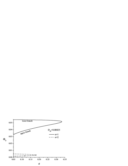
Figure 4: The shooting parameters $F^{\prime}_{0}$ and $\Phi_{0}$ as functions of the coupling parameter $a$ for soliton with $n=1$ and $n=2$, where $D_{\rm eff}=0.00025$ and $\tilde{N}=1$.

3.2 Black Holes

In the case of black holes the domain of integration is $x\in[x_{H},\infty)$, where $x_{H}$ is the dimensionless radius of the black-hole horizon. The presence of a horizon makes the black hole topologically trivial because the three-dimensional space ${\rm R}^{3}$ is equivalent to ${\rm S^{3}}$ minus a ball and the map $U(x)$ is topologically trivial. That is why the function $F$ does not have to be a multiple of $\pi$ at the black-hole horizon.

The boundary conditions at infinity are again deduced from the asymptotic flatness requirement and they are the same as in the soliton case (20). The boundary condition for the dimensionless metric function $\mu$ at the horizon is the standard one

$$\mu(x_{H})=\frac{x_{H}}{2}.$$ (23)

The regularization conditions at the horizon are

$$\left.\frac{dF}{dx}\right|_{x\rightarrow x_{H}}=\frac{\sin{2F}}{x}\frac{\left(\Phi^{2}+\frac{\sin^{2}{F}}{x^{2}}\right)}{\left(\Phi^{2}+2\frac{\sin^{2}{F}}{x^{2}}\right)}\times$$ (24)

$$\hskip 56.9055pt\times\frac{1}{1-\frac{a}{2}\sin^{2}{F}\left(2\Phi^{2}+\frac{\sin^{2}{F}}{x^{2}}\right)-x^{2}aD_{\rm eff}\left[\Phi^{4}-1+\frac{4}{\varepsilon}(1-\Phi^{\varepsilon})\right]},$$

$$\left.\frac{d\Phi}{dx}\right|_{x\rightarrow x_{H}}=\left(4x\frac{D_{\rm eff}}{\tilde{N}}(\Phi^{3}-\Phi^{\varepsilon-1})+\frac{2}{\tilde{N}}\frac{\sin^{2}{F}}{x}\Phi\right)\times$$ (25)

$$\hskip 56.9055pt\times\frac{1}{1-\frac{a}{2}\sin^{2}{F}\left(2\Phi^{2}+\frac{\sin^{2}{F}}{x^{2}}\right)-x^{2}aD_{\rm eff}\left[\Phi^{4}-1+\frac{4}{\varepsilon}(1-\Phi^{\varepsilon})\right]}.$$

Using the above boundary conditions we can conclude that in the case of the black holes we have again three shooting parameters, $A_{H}$, $F_{H}$, and $\Phi_{H}$ which denote the values of the corresponding functions on the horizon.

Like in the ESM [18], in the GSM two branches of black-hole solutions exist which we will denote by upper and lower branch. These branches are presented on Figs. 5 and 6 where the shooting parameters $F_{H}$ and $\Phi_{H}$ are plotted as functions of the radius of the horizon for sequences of black-hole solution when we vary the coupling parameters $D_{\rm eff}$ and $a$. The metric functions $\mu(x)$ and $A(x)$, the Skrymion field $F(x)$, and the scalar field $\Phi(x)$ are presented on Figs. 7 and 8 for several black-hole solutions of the lower branch with $a=0.15$, $r_{H}=0.05$ and for different $D_{\rm eff}$. The qualitative behavior of these functions is the same for the upper branch.

As it can be seen for fixed values of the coupling parameters, black-hole solutions exist up to a certain value of the radius of the horizon $x_{H}^{max}$. For fixed values of $D_{\rm eff}$, the maximal radius of the horizon $x_{H}^{max}$ decreases with the increase of $a$ and eventually reaches zero at some $a_{\rm max}$ which means that black-hole solutions do not exist for $a>a_{\rm max}$. The value of $a_{\rm max}$ for which $x_{H}^{max}$ goes to zero decreases when we increase $D_{\rm eff}$.

Like in the soliton case, the main difference between the black-hole solutions with and without scalar field is not qualitative but quantitative. The values of $x_{H}^{max}$ and $a_{\rm max}$ depend strongly on the parameter $D_{\rm eff}$ and they can be several times larger in the GSM than in the ESM. Again if we consider $D_{\rm eff}$ close to the one used in [12],[39] the values of $x_{H}^{max}$ and $a_{\rm max}$ approach the corresponding values in the ESM.

There are some interesting properties of the solutions in GSM which are also present in ESM. For fixed $D_{\rm eff}$, the $a_{\rm max}$ for black holes is the same as $a_{\rm max}$ for the $n=1$ solitons within the numerical error. When the radius of the horizon goes to zero $x_{H}\rightarrow 0$ the masses of the black holes $M$ and the values of the shooting parameters $F_{H}$ and $\Phi_{H}$ approach the values of $M$, $F_{0}$ and $\Phi_{0}$ of the corresponding $n=1$ solitons. The black-hole solutions presented so far correspond to the ground state (baryon number one) solitons. An infinite series of excitations of both the upper and the lower branches of solutions corresponding to the solitons with $n>1$ is also observed. As an example the first excitation is shown on Fig. 9 (the dashed line). As it is expected, the values of $M$, $F_{H}$ and $\Phi_{H}$ approach the corresponding values of the $n=2$ solitons when $x_{H}\rightarrow 0$. The results suggest that an infinite number of excited black-hole solutions exists and they are in one to one correspondence with the excited soliton solutions with $n>1$.

Figure 5: The shooting parameter $F_{H}$ as a function of the radius of the black-hole horizon $x_{H}$ for several values of the coupling parameters. The results for $D_{\rm eff}=0.005$ and for various values of $a$ are shown on the left panel and the results for $a=0.1$ and for various valued of the parameter $D_{\rm eff}$ are shown on the right panel.

Figure 6: The shooting parameter $\Phi_{H}$ as a function of the radius of the black-hole horizon $x_{H}$ for the same black-hole solutions as on Fig. 5 is shown.

Figure 7: The metric functions $\mu(x)$ (left panel) and $A(x)$ (right panel) for black-hole solutions with different values of $D_{\rm eff}$ ($a=0.15$ and $\tilde{N}=1$). Solutions belonging only to the lower branch of solutions are presented since the upper branch of solutions have similar qualitative behavior.

Figure 8: The skyrmion field $F(x)$ and the dilaton $\Phi(x)$ for the same black holes as on Figure 7.

Figure 9: The shooting parameters $F_{H}$ and $\Phi_{H}$ as functions of the radius of the black-hole horizon $x_{H}$ for $D_{\rm eff}=0.00025$ and $a=0.1$. Two sequences of black-hole solutions are shown where the thick line corresponds to the same black-hole solutions as the thick line on the right panels of Figs. 5 and 6, and the dashed line shows the excited black-hole solutions corresponding to the $n=2$ soliton solutions.

4 Stability and thermodynamics of the black holes

A very convenient method to infer information for the presence of instabilities in the black-hole solutions is the Poincare’s turning point method [44]. We will apply it here to prove that the lower branch of black-hole solutions is unstable. The method is based on the thermodynamics of the black holes. According to that method a change of stability is indicated by a turning point or a bifurcation point on the proper conjugate diagram. In the vicinity of a turning point the branch with a negative slope is unstable. Further details both on the formal proof and on the application of the method for the study of the stability of compact objects in gravity can be found in [45]–[50]. Some aspects of the thermodynamics of the Einstein-Skyrme black holes have been considered in [51].

The first law of thermodynamics (FLTD) for the Einstein-Skyrme black holes has been derived in [52]. A more general derivation has been given later in [53]. For the black holes studied here the FLTD has the form

$$dM=T\,dS.$$ (26)

A detailed derivation of (26) is given in Appendix A. In a micro-canonical ensemble the equilibrium solutions are the extrema of the entropy $dS=T^{-1}\,dM,$ so the conjugate variables are the mass $M$ and the inverse temperature $T^{-1}$. The conjugate diagram $T^{-1}(M)$ is given in Fig. 10 for the black-hole solutions presented on Figs. 5 and 6 (right panels).

Figure 10: The inverse temperature $T^{-1}$ as a function of the black-hole mass $M$ for sequences of black-hole solutions for different $D_{\rm eff}$ is shown.

It can be seen that the lower branch and the upper branch merge at a turning point. The slope of the lower branch on the conjugate diagram is negative which, according to the turning point method, means that the branch is unstable. It is expected that the excited black-hole solutions are dynamically unstable.

The linear stability of both the soliton and the black-hole solutions presented here is currently being investigated.

5 Conclusion

In the current paper we have studied new self-gravitating soliton and black-hole solutions in a GSM. The numerical investigation shows that the inclusion of the dilaton does not change the qualitative picture – it remains the same as in the original ESM. There are some quantitative differences, though.

For both soliton and black holes nonuniqueness of solutions is observed. If we vary the parameter $a$ and keep the rest of the parameters fixed we obtain two branches of solutions – the upper and lower branch. They merge at some maximum value $a_{\rm max}$ and no solutions are observed beyond it. The value of $a_{\rm max}$ of the solitons coincides with that of the black holes. The same coincidence is observed also in ESM. In GSM, however, $a_{\rm max}$ is highly dependent on the additional parameter $D_{\rm eff}$ which is related to the dilaton. It increases with the decrease of $D_{\rm eff}$ and may be several times higher than in the ESM.

For the black holes, if we fix $a$ and vary the radius of the event horizon $x_{H}$ the two branches merge at some maximal radius $x_{H}^{max}$. Beyond $x_{H}^{max}$ no black-hole solutions exist. Again the quantitative difference between ESM and GSM is that due to the presence of the dilaton $x_{H}^{max}$ may be considerably higher in the GSM when the same values of $a$ are considered.

In both ESM and GSM with the decrease of the radius of the horizon $r_{H}\rightarrow 0$ the masses of the black holes approach the masses of the solitons from the corresponding branch of solutions.

With the increase of the baryon number an infinite series of solitons and corresponding to them black holes exist which, however, are expected to be dynamically instable.

In the present paper we also generalize the FLTD of black-hole thermodynamics for the GSM. It has the same form as in the ESM. From the application of the turning method we inferred information for the instability of the lower branch of black holes which is in agreement with the situation in ESM.

Appendix A Derivation of the First Law of Thermodynamics

For the derivation of the first law of thermodynamics we follow the scheme in [52].

Following standard definitions for the Hawking temperature we obtain

$$T=\left.{1\over 4\pi}f\,^{\prime}A\right|_{r=r_{H}}={1\over 4\pi r_{H}}\,A(r_{H})\left(1-{1\over 2}\,v_{H}+{1\over 2}\,r_{H}^{\,2}\,V_{H}\right),$$ (27)

which together with the entropy of the horizon $S=\pi r_{H}^{2}$ gives

$$T{\partial S\over\partial r_{H}}={1\over 2}\,A(r_{H})\left(1-{1\over 2}\,v_{H}+{1\over 2}\,r_{H}^{\,2}\,V_{H}\right).$$ (28)

The mass of the black holes is given by the formula

$$M=\lim_{r\to\infty}{1\over 2}\,r\,(1-f).$$ (29)

In order to calculate the variation of the mass we will use the expression

$$r\,f\,A=\int_{r_{H}}^{r}dr^{\prime}A(r^{\prime})\left(1-{1\over 2}\,v+{1\over 2}\,r^{\prime\,2}\,V\right),$$ (30)

which can be obtained with the help of eqs. (7) and (8). Then the variation of $M$ is

$${\partial M\over\partial r_{H}}=T{\partial S\over\partial r_{H}}-{1\over 2}\int_{r_{H}}^{\infty}dr^{\prime}{\partial\over\partial r_{H}}\left[A(r^{\prime})\left(1-{1\over 2}\,v+{1\over 2}\,r^{\prime\,2}\,V\right)\right].$$ (31)

If the integral in this expression vanishes then

$${\partial M\over\partial r_{H}}=T{\partial S\over\partial r_{H}}$$

and the FLTD has the usual form

$$dM=T\,dS.$$ (32)

The integrable expression can be brought to the form of full derivative with respect to the integration variable which allows the integral to be estimated. For the derivative in the integral the Leibnitz rule gives

$${\partial\over\partial r_{H}}\left[A\,\left(1-{1\over 2}\,v+{1\over 2}\,r^{\,2}\,V\right)\right]=$$

$$\hskip 28.45274pt{\partial A\over\partial r_{H}}\left(1-{1\over 2}\,v+{1\over 2}\,r^{\,2}\,V\right)+A\,\left(-{1\over 2}\,\,{\partial v\over\partial\Phi}+{1\over 2}\,r^{\,2}\,\,{\partial V\over\partial\Phi}\right){\partial\Phi\over\partial r_{H}}$$

$$\hskip 159.3356pt+A\,\left(-{1\over 2}\,\,{\partial v\over\partial F}\right){\partial F\over\partial r_{H}}.$$ (33)

We will treat each of the terms on the right-hand side of the expression above separately. From eq. (8) we obtain

$${\partial A\over\partial r_{H}}=A\left\{{u\over r}F\,^{\prime}{\partial F\over\partial r_{H}}+a\,\tilde{N}\,r\,\Phi\,^{\prime}{\partial\Phi\over\partial r_{H}}\,+\right.\\ +\left.\int_{\infty}^{r}dr^{\prime}{\partial F\over\partial r_{H}}\left[{1\over 2r^{\prime}}\,F\,^{\prime\,2}\,{\partial u\over\partial F}-\left({u\,F\,^{\prime}\over r}\right)^{\prime}\right]+\right.\\ +\left.\int_{\infty}^{r}dr^{\prime}{\partial\Phi\over\partial r_{H}}\left[{1\over 2r^{\prime}}\,F\,^{\prime\,2}\,{\partial u\over\partial\Phi}-a\,\tilde{N}\left(r^{\prime}\Phi\,^{\prime}\right)^{\prime}\right]\right\}.$$ (34)

For the expressions in the brackets of the second term and the third term on the right-hand side from the field equations for $F$ and $\Phi$ – (9) and (10), respectively, we have that

$$-{1\over 2}\,A\,{\partial v\over\partial F}=-(f\,A\,u\,F\,^{\prime})\,^{\prime}+{1\over 2}\,f\,A\,F\,^{\prime\,2}\,{\partial u\over\partial F}$$

and

$$\,A\,\left(-{1\over 2}{\partial v\over\partial\Phi}+{1\over 2}\,r^{\,2}\,{\partial V\over\partial\Phi}\right)=-a\,\tilde{N}\,(r^{2}\,f\,A\,\Phi\,^{\prime})\,^{\prime}+{1\over 2}\,f\,A\,F\,^{\prime\,2}\,{\partial u\over\partial\Phi}.$$

Collecting all terms for the integrable we obtain

$${\partial\over\partial r_{H}}\left[A\,\left(1-{1\over 2}\,v+{1\over 2}\,r^{\,2}\,V\right)\right]=\left(\xi_{1}\xi_{2}\right)^{\prime},$$ (35)

where

$$\xi_{1}=r\,f\,A=\int_{r_{H}}^{r}dr^{\prime}A(r^{\prime})\left(1-{1\over 2}\,v+{1\over 2}\,r^{\prime\,2}\,V\right)$$ (36)

and

$$\xi_{2}=\int_{\infty}^{r}dr^{\prime}{\partial F\over\partial r_{H}}\left[{1\over 2r^{\prime}}\,F\,^{\prime\,2}\,{\partial u\over\partial F}-\left({u\,F\,^{\prime}\over r}\right)^{\prime}\right]+\\ +\int_{\infty}^{r}dr^{\prime}{\partial\Phi\over\partial r_{H}}\left[{1\over 2r^{\prime}}\,F\,^{\prime\,2}\,{\partial u\over\partial\Phi}-a\,\tilde{N}\left(r^{\prime}\Phi\,^{\prime}\right)^{\prime}\right].$$ (37)

From (35) we obtain for the integral

$$\int_{r_{H}}^{\infty}dr^{\prime}{\partial\over\partial r_{H}}\left[A(r^{\prime})\left(1-{1\over 2}\,v+{1\over 2}\,r^{\prime\,2}\,V\right)\right]=\int_{r_{H}}^{\infty}dr^{\prime}\left(F_{1}F_{2}\right)^{\prime}=\left.F_{1}F_{2}\right|_{r_{H}}^{\infty}.$$ (38)

$\xi_{2}$ is regular on the event horizon so $\left.\xi_{1}\xi_{2}\right|_{r_{H}}=0$. The situation at infinity is more subtle since $\left.\xi_{1}\right|_{\infty}\rightarrow\infty$ and $\left.\xi_{2}\right|_{\infty}\rightarrow 0$. The value of the integral at infinity can be estimated with the help of the following asymptotic expansion of the functions:

$$\left.m(r)\right|_{r\rightarrow\infty}=M-\frac{1}{2}\frac{aF_{2}^{~{}2}}{r^{3}}+{\rm O}\left(\frac{1}{r^{4}}\right),~{}\left.A(r)\right|_{r\rightarrow\infty}=1-\frac{1}{2}\frac{aF_{2}^{~{}2}}{r^{4}}+{\rm O}\left(\frac{1}{r^{5}}\right),$$ (39)

$$\left.F(r)\right|_{r\rightarrow\infty}=\frac{F_{2}}{r^{2}}+{\rm O}\left(\frac{1}{r^{3}}\right),~{}\left.\Phi(r)\right|_{r\rightarrow\infty}=1+\frac{3F_{2}^{~{}2}a}{\tilde{N}\gamma(\varepsilon-4)r^{6}}+{\rm O}\left(\frac{1}{r^{7}}\right),$$ (40)

where $F_{2}$ is a constant. With (39) and (40) it can be found that $\left.\xi_{1}\xi_{2}\right|_{\infty}\rightarrow 0$ which completes the proof of the FLTD (32).

References

- [1] G. t’Hooft , Nucl. Phys. B 72, 461, (1974); Nucl. Phys. B 75, 461, (1974).
- [2] E. Witten, Nucl. Phys. B 160, 57, (1979).
- [3] G. S. Adkins, C. R. Nappi and E. Witten, Nucl. Phys. B 228, 552, (1983).
- [4] T. H. R. Skyrme, Proc. R. Soc. A260, 127 (1961).
- [5] T. H. R. Skyrme and G. E. Brown, “Selected Papers With Commentary of Tony Hilton Royle Skyrme (World Scientific Series in 20th Century Physics, V. 3)”, World Scientific Publishing, Singapore (1994).
- [6] M. Lacombe, B. Loiseau, R. Vinh Mau and W. N. Cottingham, Phys. Rev. Lett. 57, 170 (1986).
- [7] H. Yabu, B. Schwesinger and G. Holzwarth, Phys. Lett. B 224, 25 (1989).
- [8] K. Tsushima and D. O. Riska, Nucl. Phys. A 560, 985, (1993).
- [9] G. Kälbermann and J.M. Eisenberg, Phys. Lett. B 349, 416, (1995).
- [10] A. A. Andrianov, V. A. Andrianov, Yu. V. Novozhilov and V. Yu. Novozhilov, JEPT Lett. 43, 7 (1986).
- [11] A. A. Andrianov, V. A. Andrianov, Yu. V. Novozhilov and V. Yu. Novozhilov, Phys. Lett. B 186, 401(1987).
- [12] V. Nikolaev, O. Tkachev and V. Novozhilov, Nuovo Cimento Soc. Ital. Fis. A107, 2673 (1992)
- [13] H. Luckock and I. Moss, Phys. Lett. B 176, 341 (1986).
- [14] N. Glendenning, T. Kodama and F. Klinkhamer, Phys. Rev. D38, 3226(1988).
- [15] S. Droz, M. Heusler and N. Straumann, Phys. Lett. B268, 371 (1991)
- [16] M. Heusler, S. Droz and N. Straumann, Phys. Lett. B271, 61 (1991).
- [17] M. Heusler, S. Droz and N. Straumann, Phys. Lett. B285, 21 (1992).
- [18] P. Bizon and T. Chmaj, Phys. Lett. B 297, 55 (1992).
- [19] P. Bizon, T. Chmaj and A. Rostworowski1, Phys. Rev. D75, 121702(R) (2007).
- [20] S. Zajac, Acta Phys. Polon. B40, 1617 (2009).
- [21] S. Zajac, Acta Phys. Polon. B42, 249(2011).
- [22] N. Shiiki and N. Sawado, Phys. Rev. D71, 104031 (2005).
- [23] N. Shiiki and N. Sawado, Class. Quantum Grav. 22, 3561 (2005).
- [24] B. Kleihaus, J. Kunz and A. Sood, Phys. Lett. B352, 247 (1995).
- [25] T. Torii, T. Tamaki and K. Maeda, Phys. Rev. D64, 084019 (2001).
- [26] I. Moss, N. Shiiki and E. Winstanley, Class. Quantum Grav. 17, 4161 (2000).
- [27] N. Sawado, N. Shiiki, K. Maeda and Takashi Torii, , Gen. Rel. Grav. 36, 1361 (2004).
- [28] Th. Ioannidou, B. Kleihaus and W. Zakrzewski, Phys. Lett. B600, 116 (2004).
- [29] Th. Ioannidou, B. Kleihaus and J. Kunz, Phys. Lett. B635, 161 (2006).
- [30] Th. Ioannidou, B. Kleihaus and J. Kunz, Phys. Lett. B643, 213 (2006).
- [31] B. Piette and G. Probert, Phys. Rev. D75, 125023 (2007).
- [32] G. Kälbermann, Nucl. Phys. A612, 359 (1997)
- [33] R. Ouyed and M. Butler, Astroph. J. 522, 453 (1999).
- [34] R. Ouyed, A&A 382, 939 (2002).
- [35] R. Ouyed, arXiv: astro-ph/0402122.
- [36] P. Jaikumar and R. Ouyed, Astroph. J. 639, 354 (2006).
- [37] P. Jaikumar, M. Bagchi and R. Ouyed, Astrophys. J. 678,360 (2008).
- [38] S. B. Popov and M. E. Prokhorov, A&A 434, 649 (2005).
- [39] K.E. Lassila, E.N. Magar and V.A. Nikolaev, V.Yu. Novozhilov and O.G. Tkachev, arXiv:hep-ph/0005160
- [40] M. Loewe, S. Mendizabal and J.C. Rojas, Mod. Phys. Lett. A 22, 3003 (2007).
- [41] G. S. Adkins and Ch. R. Nappi, Phys. Lett. B 137, 251 (1984).
- [42] M. Lacombe, B. Loiseau, R. Vinh Mau and W. N. Cottingham, Phys. Lett. B 169, 121 (1986).
- [43] H. Gomm, P. Jain, R. Johnson, and J. Schechter ,Phys. Rev. D33, 3476(1986).
- [44] H. Poincaré, Acta. Math. 7, 259 (1885).
- [45] R. Sorkin, Astrophys. J. 249, 254 (1981).
- [46] R. D. Sorkin, Astrophys. J. 257, 847 (1982).
- [47] T.Harada, Prog. Theor. Phys. 98, 359 (1997).
- [48] T. Torii, T. Tamaki and K. Maeda, Phys. Rev. D68, 024028 (2003).
- [49] G. Arcioni and E. Lozano-Tellechea, Phys. Rev. D72, 104021 (2005).
- [50] I. Stefanov, S. Yazadjiev and M. Todorov, Mod. Phys. Lett. A 23 (34), 2915 (2008), arXiv: 0708.4141.
- [51] T. Torii and K. Maeda, Phys. Rev. D48, 1643 (1993).
- [52] O. B. Zaslavskii, Phys. Lett. A168, 191 (1992).
- [53] M. Heusler and N. Straumann, Class. Quantum Grav. 10, 1299 (1993).