plus dijet production in the POWHEG BOX
Abstract:
We present an implementation of the calculation of the production of plus two jets at hadron colliders, at next-to-leading order (NLO) in QCD, in the POWHEG framework, which is a method that allows the interfacing of NLO calculations to shower Monte Carlo programs. This is the first process to be described to NLO accuracy within a shower Monte Carlo framework. The implementation was built within the POWHEG BOX package. We discuss a few technical improvements that were needed in the POWHEG BOX to deal with the computer intensive nature of the NLO calculation, and argue that further improvements are possible, so that the method can match the complexity that is reached today in NLO calculations. We have interfaced our POWHEG implementation with PYTHIA and HERWIG, and present some phenomenological results, discussing similarities and differences between the pure NLO and the POWHEG+PYTHIA calculation both for inclusive and more exclusive distributions. We have made the relevant code available at the POWHEG BOX web site.
1 Introduction
With the increase in energy and luminosity of the LHC, accurate predictions for high-multiplicity processes become necessary. A lot of effort has been devoted in recent years towards the calculation of next-to-leading (NLO) corrections to various and scattering processes111As usual, in this counting we do not include the decay of heavy particles. [1, 2, 3, 4, 5, 6, 7, 8, 9, 10, 11, 12, 13]. Very recently, even dominant corrections to a process have been computed [14]. When NLO predictions are available, theoretical uncertainties are reduced compared to Born level predictions, and more accurate comparisons with experimental data become possible. However, NLO predictions describe the effect due to at most one additional parton in the final state. This is quite far from realistic LHC events, which involve a large number of particles in the final state. For infrared safe, sufficiently inclusive observables, NLO calculations provide accurate predictions, but this is not the case for more exclusive observables that are sensitive to the complex structure of LHC events.
A complementary approach is provided by parton shower event generators, that generate realistic hadron-level events, but only with leading logarithmic accuracy. In recent years, methods that include the benefits of a NLO calculation together with a parton shower model (an NLO+PS generator, from now on) have become available. Using these methods one can thus generate exclusive, realistic events, maintaining NLO accuracy for inclusive observables. Two NLO+PS frameworks are being currently used in hadron collider physics: MC@NLO [15] and POWHEG [16, 17]. In the past few years a number of processes have been implemented in both frameworks. However, most processes included so far are relatively simple or scattering processes, for which the one-loop correction can be expressed in a closed, relatively simple analytic form.222Two noticeable exceptions are the POWHEG implementations of two processes: vector boson fusion Higgs production [18], and top pair production in association with one jet [19].
No process has been implemented so far in any NLO+PS framework. Tools to tackle processes of arbitrary complexity do however exist. A general computer framework for the POWHEG implementation of arbitrary NLO processes has been presented in ref. [21], the so called POWHEG BOX. Within this framework, one needs only to provide few ingredients: the phase-space and flavour information, the (spin- and colour-correlated) Born, real and virtual matrix elements for a given NLO process in order to build a POWHEG implementation of it.
Recent NLO calculations of processes of high multiplicity use numerical methods to perform the reduction of tensor integrals “on the fly” or to compute coefficients of master integrals in terms of products of tree-level amplitudes. These methods allow the computation of the virtual corrections to very complex processes. On the other hand, these calculations become quite computer intensive. The computation of real radiation corrections also requires a considerable CPU time, since one needs to integrate over a phase space of high dimension. For instance, if on shell particles are produced at Born level, the real radiation term involves an integration over variables.
In this paper we present a POWHEG BOX implementation of the QCD production of +2 jets, including the leptonic decay of the bosons with spin correlations. This is the first time that a process has been implemented in an NLO+PS framework. NLO QCD corrections to production have been computed recently using -dimensional unitarity [12]. The production of a pair in hadronic collisions requires the presence of two jets in the final state. Thus, in spite of the presence of the these jets, there are no collinear or soft divergences at the Born level. As such, the process presents no complications due to the need of a generation cut [23]. However, since the NLO calculation is computer intensive, a number of technical issues arise in POWHEG that are not present for simpler processes. We discuss some of these issues in the present work, and find acceptable solutions for some of them. We also show that further efficiency improvements are possible, thus paving the road for the matching of NLO calculations and parton showers for yet more complex processes.
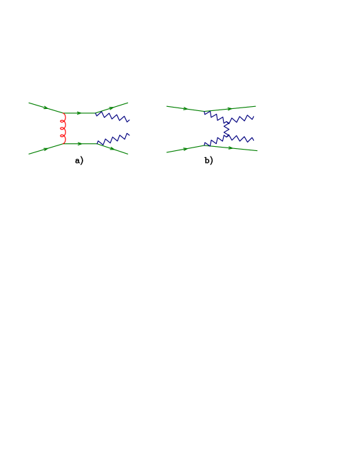
We consider in this work only the QCD production mechanism of the +2 jets final state, i.e. the process involving one gluon exchange and the direct emission of the pair from quark lines (see fig. 1a). A different production mechanism is given by the electroweak (EW) scattering process, where a colourless vector boson is exchanged in the -channel (see fig. 1b). This second mechanism, although of higher order in the electroweak coupling constant, is only moderately smaller than the QCD one. We leave the POWHEG implementation of the EW production process, for which NLO QCD corrections are also known [22], to a future publication.
The +2 jets process has a considerable phenomenological interest. It’s LHC cross section, including the branching ratios to electrons and muons, is around fb at TeV and fb at TeV. It has a distinct signature of two same-sign leptons, missing energy and two jets. It therefore constitutes an important background to studies of double-parton scattering [24], as well as to new physics signatures that involve two same-sign leptons, such as R-parity violating SUSY models [25], diquark production with decay of the diquark to a pair of top quarks [26] or double charged Higgs production [27]. This work will make it possible to have a more reliable generator of this SM background in those physics studies, that currently use only LO (Leading Order) shower Monte Carlo programs.
The remainder of this paper is organized as follows. In section 2 we discuss the process under study. In section 3 we present few technical issues related to the implementation of the process in the POWHEG BOX [21] (more details are given in appendix A). In section 4 we present physical results for some kinematic distributions. We pay particular attention to where NLO results differ mostly from the POWHEG ones. We draw our conclusions and outlook in section 5.
2 plus dijet production
The process + 2 jets has been computed at NLO in [12], and we fully use those results here. In this section we recall few aspects of the calculation and refer the reader to [12] for all other details.
For the one-loop calculation one expresses one-loop amplitudes as a linear combination of master integrals and uses -dimensional unitarity to compute the coefficients of the master integrals in this decomposition of the amplitude. The coefficients are then given by products of tree-level amplitudes evaluated in higher dimensions and involving complex momenta. These tree-level helicity amplitudes are evaluated using recursive Berends-Giele relations[28]. This is the most natural choice since recursion relations can be easily used to compute amplitudes involving complex momenta in an arbitrary dimension. The master integrals are evaluated using the package QCDloop[20].
The ingredients needed to implement a new process in the POWHEG BOX are then [21]
-
•
the list of the flavour structures in the Born and real processes for incoming and outgoing particles. Only one flavour structure must appear for each class of flavour structures that are equivalent up to a permutation of final state particles. In the present case we have 20 flavour structures for the Born and 36 for the real radiation contributions;
-
•
the Born phase space. In our case the Born phase space involves an integration over 16 variables (of which one azimuthal angle is irrelevant);
-
•
the Born, real and virtual squared matrix elements. Furthermore, one needs the Born colour and spin-correlated amplitudes. The last one arises only if there are gluons as external particles, which is not the case in our process. The colour correlated Born amplitudes are available in the code of ref. [12], where they are used in the computation of the virtual amplitudes. The matrix elements for each flavour structure should be appropriately symmetrized if identical particles appear in the final state;
-
•
the Born colour structures in the limit of large number of colours. Once the POWHEG event kinematics and flavour structure is generated, we must also assign a planar colour structure to it, that is needed by the shower program for building the subsequent radiation and to model the hadronization process. In POWHEG this colour assignment is based upon the colour structure of the Born term in the planar limit[21]. In the process at hand, we have two possibilities. In the case of two quark pairs of distinct flavour, there is at Born level only one diagram, therefore the leading colour structure is fixed. In the case of identical fermions there are two diagrams at Born level, corresponding to and channel scattering. We pick then the leading colour structure for each phase space point according to the value of the squared matrix element for and channel scattering, neglecting the interference term.
We performed the following checks on the implementation of the NLO calculation:
-
•
The POWHEG BOX computes internally the soft and collinear limits of the real amplitude, using only the Born cross section. These are compared to the full real amplitude in the soft and collinear limits, and the results of this comparison are written to a file. This is a valuable check on the real and Born amplitudes, and is performed automatically by the POWHEG BOX.
-
•
The POWHEG BOX can also be used to compute bare LO and NLO distributions. Using this feature, by fixing the same input as in [12], we have verified that we reproduce all LO and NLO cross-sections and distributions presented there.
3 Technical details in POWHEG
In this section we discuss some technical issues having to do with the POWHEG implementation of the +2 jets process. We assume that the reader has some familiarity with the POWHEGmethod.
At the beginning, the POWHEG BOX computes the integral of the so called function. The , that we denote collectively with , are a set of variables (where is the number of final state particles in the real emission process, including decay products), defined in the unit cube, that parametrize the momentum fraction of the incoming partons and the full phase space for real emission. More specifically, the first variables, denoted collectively as , parametrize the underlying Born configuration, while the last three variables, denoted by , parametrize the radiation. The integral
| (1) |
represents the inclusive cross section for the process in question at fixed underlying Born configuration. POWHEG produces events by first generating the underlying Born configuration, and then generating radiation using a shower technique.
The and function are sum of terms, each term referring to a specific flavour structure of the underlying Born. POWHEG first computes the integral and an upper bounding envelope of the function. Using this upper bounding envelope, it is possible to generate the variables with a probability distribution proportional to using a hit and miss technique. The values are discarded, and the remaining variables are thus generated with a probability proportional to . The flavour structure of the underlying Born configuration is chosen with a probability proportional to each flavour component of at the generated point. The function itself is the sum of the Born and the virtual contributions evaluated at the underlying Born phase space configuration, plus an appropriate combination of the real emission cross section, the soft and collinear subtractions, and the collinear remnants from the subtraction of the initial state singularities. This combination also depends upon the variables, while the Born and virtual contributions do not. The evaluation of the function requires a calculation of the total virtual cross section for each flavour configuration. It turns out that one evaluation of the function requires a time of the order of 30 seconds.333This is the typical time on a 2.4 GHz CPU, if the program is compiled with the ifort compiler. Although this seems to be a fairly long time, as long as the problem can be trivially parallelized on a large CPU cluster, it can be dealt with. In fact, however, the problem can be parallelized only after the importance sampling integration grid has been established. It is thus common practice, in this kind of NLO calculations, to build the adaptive integration grid using only the Born contribution. In our case, we introduced a switch in our input file, called fakevirt. If this token is set to one, the virtual correction is replaced by a term proportional to the Born cross section. We thus perform the first integration step, when the adaptive integration grid is formed, with this token set, so that no calls to the virtual routines are performed. This way, it is not difficult to obtain reasonably looking adaptive grids with 500000 calls to the function, taking about 10 hours of CPU time. The same calculation using the full virtual contribution would take a time of the order of 170 days, and would thus be unfeasible.
After the importance sampling grid has been established, the computation of the integral of the function, and the computation of the upper bounding envelope that is used for the generation of the underlying Born configurations, can be performed in parallel. The POWHEG BOX already had a mechanism to perform this stage of the computation in parallel and to combine all the results.
We have found that it is convenient to use the so called “folding” technique in the integration of the function. The folding procedure is better explained by an example. Given a function to be integrated by a Monte Carlo technique in the range , one can replace it by the function
| (2) |
also defined for . It is obvious that
| (3) |
It is also obvious that the larger is, the smoother the function will be, thus requiring less points in a Monte Carlo integration. We call this procedure “folding” the variable. In the POWHEG BOX, the radiation variables can be folded individually.444In fact, rather than the variables, what is folded are the corresponding variables, piecewise linear functions of the , that have constant importance sampling in the adaptive grid. In previous works, the use of folding was advocated to avoid spurious negative weights. In the present case, besides also serving that purpose, folding is used to balance the computer time needed for the computation of the real and virtual contribution. In fact, since only the radiation variables are folded, the virtual contribution is the same in a given folded set, and thus is computed only once. The real contribution is instead computed several times. By using this procedure, the function becomes a smoother function of the radiation variables, so that the integration becomes easier to perform, and also the generation of the underlying Born configurations becomes more efficient. It is found that with folding numbers of 5, 5, 10, referring respectively to the radiation variables , and , the time required to compute the virtual contribution becomes comparable to the time for the evaluation of the real one. As we said earlier, by using the Intel Fortran compiler, the time for a single call to the virtual cross section is roughly 30 seconds. In order to get 500000 points, one needs about 170 days of computer time, a relatively easy task on modern days clusters with hundreds of CPU’s. A further problem arises, however. Assuming that we are using 100 CPU’s, each process generates 5000 points. This is not enough to get a reasonable upper bounding envelope for the generation of the underlying Born configuration. In fact, the procedure used in the POWHEG BOX (described in ref. [29]) has no time to reach the upper bound with such a small number of points. Even when combining together the upper bounds of the different runs, one gets an unacceptable rate of upper bound failures in the generation of the underlying Born configuration, of the order of 1 every ten calls to the function, which can thus affect final distributions. We modified the POWHEG BOX basic code, in order to deal with this problem. In short, the return values of the function calls were first written to files by the parallel processes, and the upper bounding envelope was later evaluated by reading all the generated files. After this step, the program is capable of generating user process events (that is to say, events ready to be fed through a shower Monte Carlo program). The efficiency, however, turns out to be very small, of the order of 2%. This means that the generation time is of the order of seconds, roughly a couple of events per hour. In order to collect 100000 events, we would thus need 500 hours on a typical 100 CPU’s cluster. We were able to reach 15% efficiency by a further technical modification to the POWHEG BOX code which is described in appendix A.
At this point, no further problems arise. One can generate the upper bound normalization for the generation of radiation, and start the event generation using a parallel CPU cluster. The upper bound failures in the generation of the underlying Born configurations are at the level of 2 for 1000 generated events. Due to the large folding numbers, the fraction of negative weighted events is only 0.4%, an acceptable value. The generation time is about three minutes per event. Most of the generation time is consumed by the computation of . Since the efficiency in the generation of the underlying Born is of the order of 10%, the generation time is of the order of several times the time needed for the computation of a single virtual point. Again, having a large CPU cluster at one’s disposal, it is not hard to generate few hundred thousands events.
It is also worth asking whether other improvements in performance are actually possible. Aside from considering more aggressive hardware requirements, like using GPU’s and the like, we have immediately noted another speed aspect that can be improved by modifying suitably the POWHEG BOX code. In fact, at the moment, we compute the full function when we generate the underlying Born kinematics, and decide its flavour structure on the basis of the size of each flavour contribution to it. This is what was implemented in the POWHEG BOX, mainly for reasons of simplicity. A more efficient approach would be to store sufficient information to generate each underlying Born flavour configuration individually. In this way, the generation process would start by picking an underlying Born flavour configuration with probability proportional to the corresponding contribution to the total cross section. Given the underlying Born flavour configuration, one would then generate the underlying Born phase space. It is not unlikely that, with this approach, one may gain a factor of order 10 in speed.
Alternatively, a speed gain may be achieved if the code that computes the virtual contribution is optimized to compute all flavour structure contributions to the virtual cross section at once.
4 Results
In this section we present our results. We consider proton-proton collisions with center-of-mass energy . We require the bosons to decay leptonically into . The -bosons are produced on mass-shell and we assume a diagonal CKM matrix. Neglecting interference effects, which are numerically suppressed since they force the bosons off mass-shell, the cross-section for same-flavour production is half that of different flavour. This implies that the full cross-section summing over electrons and muons can be obtained by multiplying the results presented here by a factor two.
The setup used is largely inspired by [12], but we consider here a different center of mass energy. In the distributions shown, we impose the following leptonic cuts
| (4) |
We define jets using the anti- algorithm [30], with the parameter set to 0.4. We do not impose any transverse-momentum cut on the two outgoing jets, nor do we impose lepton isolation cuts.
The mass of the -boson is taken to be , the width GeV. couplings to fermions are obtained from and . We use MSTW08NLO parton distribution functions, corresponding to [31]. We consider the top quark infinitely heavy and neglect its effects, while all other quarks are treated as massless. We set the factorization scale equal to the renormalization scale, which we choose to be
| (5) |
where , and and are the transverse momenta of the two and of the two emitted partons in the underlying Born configuration. We use PYTHIA 6.4.21 [32] to shower the events, include hadronization corrections and underlying event effects, with the Perugia 0 tune (i.e. we call PYTUNE(320) before calling PYINIT). We have also showered the events using HERWIG [33]. We found only marginal differences between the HERWIG and PYTHIA results. Thus, we do not show any plot of HERWIG results.
We remind the reader that we consider here only the QCD production of , while we completely neglect the electroweak production. We also stress that we have not computed any theoretical error due to scale variations or PDF uncertainties on our distributions. Thus, our error bars are only statistical. The purpose of the plots we show is only to validate our results. Since the code is public, a user may study theoretical uncertainties at will.
With the setup described above, we obtain an NLO total cross-section of fb, that coincides by construction with the POWHEG+PYTHIA result. If we impose the leptonic cuts of eq. (4), and do not require any minimum transverse momentum for the jets, we have a NLO cross section of fb, and a slightly lower cross section with POWHEG+PYTHIA of fb. Unless otherwise stated, these are the cuts applied to the distributions presented in the following. If we also require to have at least two jets with transverse momentum larger than GeV we obtain an NLO inclusive cross-section of fb. A GeV transverse momentum cut was also applied to the third hardest jet, when we plot its rapidity distribution.
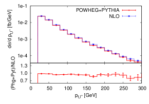
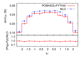
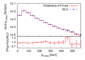
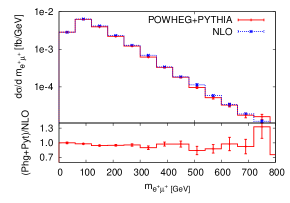
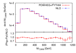
We now discuss some kinematical distributions. We first consider leptonic inclusive distributions. We plot in fig. 2 the inclusive transverse momentum distribution for the charged lepton ( or ) and its rapidity distribution , the missing transverse momentum, the charged lepton system invariant mass , and the transverse mass of the two bosons defined as
| (6) |
where the missing transverse energy is reconstructed from the missing transverse momentum using the invariant mass of the charged lepton system . For these distributions we find good agreement between NLO and POWHEG+PYTHIA, and do not observe any relevant difference in shape.
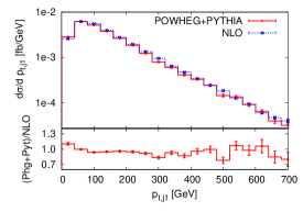
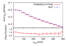
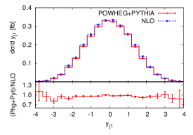
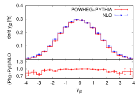
In fig. 3 we show some hadronic inclusive distributions. We plot the transverse momentum and rapidity distributions of the two leading jets, i.e. those with largest transverse momentum, and the total transverse energy of the event , defined as
| (7) |
where the sum runs over all jets in the event. For the transverse momentum and rapidity distributions we notice differences of the order of 10% between the NLO and POWHEG+PYTHIA results. We also find that the POWHEG+PYTHIA distributions tend to be more peaked for smaller jet transverse momenta, and also that jets tend to be slightly more central.
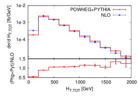
The distribution, on the other hand, displays large differences, especially on the first bin, where the POWHEG+PYTHIA result is a factor 2 smaller that the NLO one. This feature is easily explained. The shower and the underlying event generated by PYTHIA adds several soft particles to the event. Since we do not apply any transverse momentum cut, these soft particles are clustered in jets, and contribute positively to . Because of the large multiplicity of LHC events, assuming a typical transverse momentum of 500 MeV for soft hadrons, we see that it is not inconceivable that this increase may reach values of the order of 50 GeV. The first bin of the distribution is the most affected one, because this mechanism can cause events to migrate to higher bins from it, while no event will migrate backward. This explanation is easily tested. First of all, we show in the left plot of fig. 4 that the POWHEG user process event, without PYTHIA shower, is in good agreement with the NLO result.
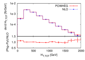
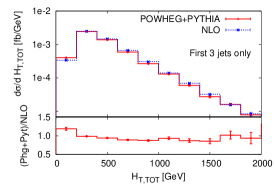
We see that, if anything, it is the POWHEG distribution that is slightly above the NLO one. This proves that this feature is not originated by the POWHEG implementation. In the right plot, we show a comparison of the POWHEG+PYTHIA and the NLO calculation for the distribution, this time defined to involve only the three hardest jets. The NLO distribution, of course, is not affected. On the other hand, the POWHEG+PYTHIA is brought in much better agreement with the NLO calculation.
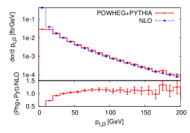
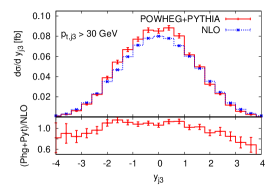
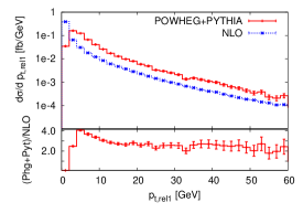
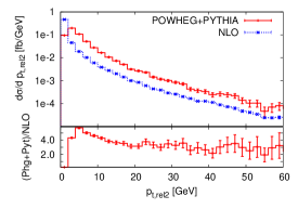
Finally, we show in fig. 5 the transverse momentum and rapidity of the third jet (in the last distribution we impose a transverse momentum cut of 30 GeV on the jets), and the relative transverse momentum distribution of the particles inside the two leading jets defined with respect to the jet axis in the frame where the jet has zero rapidity
| (8) |
Here denotes the momentum of the particle and of the jet. At NLO it is only the real radiation that contributes to these four distributions, and we see clearly a divergence at small and , while in the POWHEG+PYTHIA prediction the distribution has a Sudakov peak and goes to zero for . We also remark that the third jet tends to be more central with POWHEG+PYTHIA.
5 Conclusions
In this work we have presented a POWHEG implementation for the QCD production of plus two jets, at NLO in the strong coupling constant, with leptonic decays included with NLO accurate spin correlations. The NLO corrections for this process have been computed recently using -dimensional unitarity in ref. [12]. In this work we just focused upon building up a POWHEG implementation, in order to consistently interface the calculation to shower Monte Carlo generators. The POWHEG implementation was built in the framework of the POWHEG BOX [21].
The process is of considerable phenomenological interest, being an important background to new physics signatures, and to the study of double parton scattering phenomena. Furthermore, its study is also interesting since it represents a first POWHEG implementation of a complex, scattering process, where the calculation of the virtual corrections is highly demanding from a computational point of view. Besides this issue, the POWHEG implementation of this process does not present any special problem. The Born cross section is finite, in spite of the presence of the two jets in the final state, so, from this point of view the process is similar to Higgs boson production in Vector Boson Fusion [18]. However, the large amount of computer time required for the calculation of the virtual contributions has in practice turned out into a difficult problem to deal with, so that the POWHEG BOX implementation of the process was in fact not completely trivial.
We have spotted a number of possible improvements to the POWHEG BOX code that can result in a substantial increase in efficiency, and we have implemented the most simple ones. We were thus able to generate an adequate number of events for this process and, most importantly, we have convinced ourselves that the POWHEG BOX efficiency can be increased even further, in order to match the level of complexity that is now possible in NLO calculations.
We have compared the POWHEG BOX result, interfaced with the PYTHIA and HERWIG Monte Carlo, with the bare NLO one, and have found consistency with the features observed in other implementations: very inclusive observables, like the lepton spectra, display a remarkable agreement; quantities involving leading jets also agree well, with only minor differences; quantities involving the radiated jet display marked differences in the Sudakov region.
Finally, we have made our code public. It can be retrieved by following the instructions at the POWHEG BOX web site http://powhegbox.mib.infn.it.
Acknowledgments We thank Kirill Melnikov, Carlo Oleari and Emanuele Re for useful exchanges. The calculations have been performed using TURING, the INFN computer cluster in Milano-Bicocca, and the centralized INFN CSN4Cluster. This work is supported by the British Science and Technology Facilities Council and by the LHCPhenoNet network under the Grant Agreement PITN-GA-2010-264564.
Appendix A Raising the generation efficiency
Due to the large amount of computer time needed to compute virtual corrections, it is mandatory to increase the generation efficiency for the underlying Born configurations. For processes with many external legs, this efficiency can be in fact quite low.
The POWHEG BOX generates the underlying Born and radiation kinematics using a hit and miss technique. An upper bounding envelope of the function is found, of the form
| (9) |
where the are the integration variables, and the functions are step functions of the integration variables. The size of the step is determined by the importance sampling grid itself, as documented in ref. [29]. In order to generate a configuration, the points are first generated with a probability distribution equal to . Then a uniform random number , with
| (10) |
is generated. One then computes . If we have a hit, and the configuration is kept. Otherwise the configuration is rejected (we have a miss), and we restart the procedure.
It is clear that, if the number of integration variables is large (as in our case), an upper bound of the form eq. (9) will generally be highly inefficient, just because the product of a large number of terms will tend to build up large values. In order to remedy to this problem, we have exploited the fact that the function is equal to the Born cross section plus higher order terms. It is thus natural to expect that an upper bound of the form
| (11) |
will be much closer to it. We thus determine the functions for this bound, using the same technique used for the functions. Then we modified our code in such a way that, before computing in order to test for a hit or miss, we compute the right hand side of eq. (11). If it is smaller than , will also be smaller than , and we thus know that we have a miss without the need to compute the time consuming function. By adopting this method, we have reached an efficiency of 15%, instead of a 1-2% efficiency that we achieve with the POWHEG BOX default method.
References
- [1] A. Bredenstein, A. Denner, S. Dittmaier, S. Pozzorini, Phys. Rev. Lett. 103 (2009) 012002. [arXiv:0905.0110 [hep-ph]].
- [2] A. Bredenstein, A. Denner, S. Dittmaier, S. Pozzorini, JHEP 1003 (2010) 021. [arXiv:1001.4006 [hep-ph]].
- [3] G. Bevilacqua, M. Czakon, C. G. Papadopoulos, R. Pittau, M. Worek, JHEP 0909 (2009) 109. [arXiv:0907.4723 [hep-ph]].
- [4] C. F. Berger et al., Phys. Rev. Lett. 102 (2009) 222001. [arXiv:0902.2760 [hep-ph]].
- [5] C. F. Berger et al., Phys. Rev. D80 (2009) 074036. [arXiv:0907.1984 [hep-ph]].
- [6] R. K. Ellis, K. Melnikov, G. Zanderighi, JHEP 0904 (2009) 077. [arXiv:0901.4101 [hep-ph]].
- [7] R. K. Ellis, K. Melnikov, G. Zanderighi, Phys. Rev. D80 (2009) 094002. [arXiv:0906.1445 [hep-ph]].
- [8] K. Melnikov, G. Zanderighi, Phys. Rev. D81 (2010) 074025. [arXiv:0910.3671 [hep-ph]].
- [9] T. Binoth, N. Greiner, A. Guffanti, J. Reuter, J. -P. .Guillet, T. Reiter, Phys. Lett. B685 (2010) 293-296. [arXiv:0910.4379 [hep-ph]].
- [10] G. Bevilacqua, M. Czakon, C. G. Papadopoulos, M. Worek, Phys. Rev. Lett. 104 (2010) 162002. [arXiv:1002.4009 [hep-ph]].
- [11] C. F. Berger et al., Phys. Rev. D82 (2010) 074002. [arXiv:1004.1659 [hep-ph]].
- [12] T. Melia, K. Melnikov, R. Rontsch, G. Zanderighi, JHEP 1012 (2010) 053. [arXiv:1007.5313 [hep-ph]].
- [13] A. Denner, S. Dittmaier, S. Kallweit et al., [arXiv:1012.3975 [hep-ph]].
- [14] C. F. Berger et al., [arXiv:1009.2338 [hep-ph]].
- [15] S. Frixione, B. R. Webber, JHEP 0206 (2002) 029. [hep-ph/0204244].
- [16] P. Nason, JHEP 0411 (2004) 040. [hep-ph/0409146].
- [17] S. Frixione, P. Nason, C. Oleari, JHEP 0711 (2007) 070. [arXiv:0709.2092 [hep-ph]].
- [18] P. Nason, C. Oleari, JHEP 1002 (2010) 037. [arXiv:0911.5299 [hep-ph]].
- [19] A. Kardos, C. Papadopoulos and Z. Trócsányi, arXiv:1101.267v1 [hep-ph].
- [20] R. K. Ellis, G. Zanderighi, JHEP 0802 (2008) 002. [arXiv:0712.1851 [hep-ph]].
- [21] S. Alioli, P. Nason, C. Oleari and E. Re, JHEP 1006 (2010) 043. [arXiv:1002.2581 [hep-ph]].
- [22] B. Jager, C. Oleari, D. Zeppenfeld, Phys. Rev. D80 (2009) 034022. [arXiv:0907.0580 [hep-ph]].
- [23] S. Alioli, P. Nason, C. Oleari, E. Re, JHEP 1101 (2011) 095. [arXiv:1009.5594 [hep-ph]].
-
[24]
A. Kulesza, W. J. Stirling,
Phys. Lett. B475 (2000) 168-175.
[hep-ph/9912232];
E. Maina, JHEP 0909 (2009) 081. [arXiv:0909.1586 [hep-ph]];
J. R. Gaunt, C. -H. Kom, A. Kulesza, W. J. Stirling, Eur. Phys. J. C69 (2010) 53-65. [arXiv:1003.3953 [hep-ph]]. - [25] H. K. Dreiner, S. Grab, M. Kramer, M. K. Trenkel, Phys. Rev. D75 (2007) 035003. [hep-ph/0611195].
- [26] T. Han, I. Lewis, T. McElmurry, JHEP 1001 (2010) 123. [arXiv:0909.2666 [hep-ph]].
- [27] J. Maalampi, N. Romanenko, Phys. Lett. B532 (2002) 202-208. [hep-ph/0201196].
- [28] F. A. Berends, W. T. Giele, Nucl. Phys. B306 (1988) 759.
- [29] P. Nason, [arXiv:0709.2085 [hep-ph]].
- [30] M. Cacciari, G. P. Salam, G. Soyez, JHEP 0804 (2008) 063. [arXiv:0802.1189 [hep-ph]].
- [31] A. D. Martin, W. J. Stirling, R. S. Thorne, G. Watt, Eur. Phys. J. C63 (2009) 189-285. [arXiv:0901.0002 [hep-ph]].
- [32] T. Sjostrand, S. Mrenna, P. Z. Skands, JHEP 0605 (2006) 026. [hep-ph/0603175].
- [33] G. Corcella et al., JHEP 0101 (2001) 010. [hep-ph/0011363].