Periodic orbits for classical particles having complex energy

Abstract

This paper revisits earlier work on complex classical mechanics in which it was argued that when the energy of a classical particle in an analytic potential is real, the particle trajectories are closed and periodic, but that when the energy is complex, the classical trajectories are open. Here it is shown that there is a discrete set of eigencurves in the complex-energy plane for which the particle trajectories are closed and periodic.

I Introduction

This paper continues and advances the ongoing research program to extend conventional real classical mechanics into the complex domain. Complex classical mechanics is a rich and largely unexplored area of mathematical physics, and in the current paper we report some new analytical and numerical discoveries.

In past papers on the nature of complex classical mechanics, many analytic potentials were examined and some unexpected phenomena were discovered. For example, in numerical studies it was shown that a complex-energy classical particle in a double-well potential can exhibit tunneling-like behavior R1 . Multiple-well potentials were also studied and it was found that a complex-energy classical particle in a periodic potential can exhibit a kind of band structure R2 . It was surprising to find classical-mechanical systems that can exhibit behaviors that one would expect to be displayed only by quantum-mechanical systems.

In previous numerical studies it was also found that the complex classical trajectories of a particle having real energy are closed and periodic, but that the classical trajectories of a particle having complex energy are generally open. The claim that classical orbits are closed and periodic when the energy is real and that classical orbits are open and nonperiodic when the energy is complex was first made in Ref. R3 and was examined numerically in Ref. R1 . In these papers it was emphasized that this property is consistent with the Bohr-Sommerfeld quantization condition

$$\oint_{C}dx\,p=\left(n+\textstyle{\frac{1}{2}}\right)\pi,$$ (1)

which can only be applied if the classical orbits are closed. Thus, there seems to be an association between real energies and the existence of closed classical trajectories R4 .

However, in this paper we show analytically that while a classical particle having complex energy almost always follows an open and nonperiodic trajectory, there is a special discrete set of curves in the complex-energy plane for which the classical orbits are actually periodic. We call these curves eigencurves because the requirement that the trajectory of a classical particle having complex energy be closed and periodic is a kind of quantization condition that specifies a countable set of curves in the complex-energy plane. When the energy of a classical particle lies on an eigencurve, the trajectory of the particle in the complex coordinate plane is periodic.

This paper is organized as follows: In Sec. II we give a brief review of complex classical mechanics focusing on the tunneling-like behavior of a classical particle that has complex energy. In Sec. III we describe the special periodic orbits of a complex classical particle in a quartic double-well potential. In Sec. IV we consider sextic and octic potentials. Finally, in Sec. V we make some brief concluding remarks.

II Background and Previous Results on Tunneling-like behavior in Complex Classical Mechanics

For the past twelve years there has been an active research program to extend quantum mechanics into the complex domain. Complex quantum mechanics has rapidly developed into a rich and exciting area of physics. It has been found that if the requirement that a Hamiltonian be Hermitian is weakened and broadened to include complex non-Hermitian Hamiltonians that are ${\cal P}{\cal T}$ symmetric, some of the quantum theories that result are physically acceptable because these Hamiltonians possess two crucial features: (i) their eigenvalues are all real, and (ii) they describe unitary time evolution. (A Hamiltonian is ${\cal P}{\cal T}$ symmetric if it is invariant under combined spatial reflection ${\cal P}$ and time reversal ${\cal T}$ R5 ; R6 .) Such Hamiltonians have been observed in laboratory experiments R7 ; R8 .

The study of complex classical mechanics arose in an effort to understand the classical limit of complex quantum theories. In the study of complex classical systems, the complex as well as the real solutions to Hamilton’s differential equations of motion are considered. In this generalization of conventional classical mechanics, classical particles are not constrained to move along the real axis and may travel through the complex plane.

Early work on the particle trajectories in complex classical mechanics is reported in Refs. R9 ; R10 . Subsequently, detailed studies of the complex extensions of various one-dimensional conventional classical-mechanical systems were undertaken: The remarkable properties of complex classical trajectories are examined in Refs. R11 ; R12 ; R13 ; R14 ; R15 . Higher dimensional complex classical-mechanical systems, such as the Lotka-Volterra equations for population dynamics and the Euler equations for rigid body rotation, are discussed in Refs. R3 . The complex ${\cal P}{\cal T}$-symmetric Korteweg-de Vries equation has also been studied R16 ; R17 ; R18 ; R19 ; R20 ; R21 ; R22 .

In part, the motivation for extending classical mechanics into the complex domain is that doing so might enhance one’s understanding of the subtle mathematical phenomena that real physical systems can exhibit. For example, some of the complicated properties of chaotic systems become more transparent when extended into the complex domain R23 . Second, studies of exceptional points of complex systems have revealed interesting and potentially observable effects R24 ; R25 . Third, recent work on the complex extension of quantum probability density constitutes an advance in understanding the quantum correspondence principle R26 . Fourth, and most relevant to the work in this paper, is the prospect of understanding the nature of tunneling.

Let us illustrate how a classical particle can exhibit tunneling-like behavior. Consider a classical particle in the quartic double-well potential $V(x)=x^{4}-5x^{2}$. Figure 1 shows eight complex classical trajectories for a particle of real energy $E=-1$. Each of these trajectories is closed and periodic. Observe that for this energy the trajectories are localized either in the left well or the right well and that no trajectory crosses from one side to the other side of the imaginary axis.

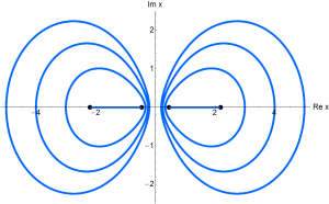
Figure 1: Eight classical trajectories in the complex-$x$ plane representing a particle of energy $E=-1$ in the potential $x^{4}-5x^{2}$. The turning points are located at $x=\pm 2.19$ and $x=\pm 0.46$ and are indicated by dots. Because the energy is real, the trajectories are all closed. The classical particle stays in either the right-half or the left-half plane and cannot cross the imaginary axis. Thus, when the energy is real, there is no effect analogous to tunneling.

What happens if we allow the classical energy to be complex R1 ? In this case the classical trajectory is generally not closed, but surprisingly it also does not spiral out to infinity. Rather, the trajectory in Fig. 2 unwinds around a pair of turning points for a characteristic length of time and then crosses the imaginary axis. At this point the trajectory does something remarkable: Rather than continuing its outward journey, it spirals inward towards the other pair of turning points. Then, never intersecting itself, the trajectory turns outward again, and after the same characteristic length of time, returns to the vicinity of the first pair of turning points. This oscillatory behavior, which shares the qualitative characteristics of strange attractors, continues forever but the trajectory never crosses itself. As in the case of quantum tunneling, the particle spends a long time in proximity to a given pair of turning points before rapidly crossing the imaginary axis to the other pair of turning points. On average, the classical particle spends equal amounts of time on either side of the imaginary axis. Interestingly, we find that as the imaginary part of the classical energy increases, the characteristic “tunneling” time decreases in inverse proportion, just as one would expect of a quantum particle.

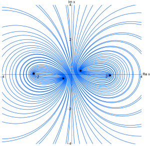
Figure 2: Classical trajectory of a particle moving in the complex-$x$ plane under the influence of a double-well $x^{4}-5x^{2}$ potential. The particle has complex energy $E=-1-i$ and its trajectory does not close. The trajectory spirals outward around one pair of turning points, crosses the imaginary axis, and then spirals inward around the other pair of turning points. It then spirals outward again, crosses the imaginary axis, and goes back to the original pair of turning points. The particle repeats this behavior endlessly but at no point does the trajectory cross itself. This classical-particle motion is analogous to the behavior of a quantum particle that repeatedly tunnels between two classically allowed regions. Here, the particle does not disappear into the classically forbidden region during the tunneling process; rather, it moves along a well-defined path in the complex-$x$ plane from one well to the other.

The measurement of a quantum energy is inherently imprecise because of the time-energy uncertainty principle $\Delta E\,\Delta t\gtrsim\hbar/2$. Specifically, since there is not an infinite amount of time in which to make a quantum energy measurement, the uncertainty in the energy $\Delta E$ is nonzero. In Ref. R1 the uncertainty principle was generalized to include the possibility of complex uncertainty: If we suppose that the energy uncertainty $\Delta E$ has a small imaginary component, then in the corresponding classical theory, while the particle trajectories are almost periodic, the orbits do not close exactly. The fact that the complex-energy classical orbits are not closed means that in complex classical mechanics one can observe tunneling-like phenomena that one normally expects to find only in quantum systems.

III Periodic orbits in a quartic double-well potential

Let us consider the complex motion of a classical particle in the double-well potential

$$V(x)=x^{4}-5x^{2}.$$ (2)

In general, the trajectory $x(t)$ of a classical particle in a potential $V(x)$ satisfies the differential equation

$$[x^{\prime}(t)]^{2}+V(x)=E,$$ (3)

which is obtained by integrating Hamilton’s equations of motion once. This differential equation is separable, and for the double-well potential in (2) the equation may be written as

$$dt=\frac{dx}{\sqrt{E+5x^{2}-x^{4}}}.$$ (4)

Integrating both sides of (4) gives rise to a Jacobi elliptic function. The standard Jacobi elliptic function ${\rm sn}(u,k)$ is defined implicitly in terms of the integral:

$$u=\int_{0}^{{\rm sn}(u,k)}\frac{ds}{\sqrt{(1-s^{2})(1-k^{2}s^{2})}}.$$ (5)

It is well known that the Jacobi elliptic function is doubly periodic and that it satisfies the double periodicity condition

$${\rm sn}[u+2mK(k)+2niK(k^{\prime}),k]=(-1)^{m}{\rm sn}(u,k),$$ (6)

where $m$ and $n$ are integers, $K(k)$ is the complete elliptic integral

$$K(k)\equiv\int_{0}^{1}\frac{ds}{\sqrt{(1-s^{2})(1-k^{2}s^{2})}},$$ (7)

and $k^{\prime}\equiv\sqrt{1-k^{2}}$.

To identify the value of $k$ for the particular differential equation in (4), we must factor the polynomial $E+5x^{2}-x^{4}$. Note that this polynomial has four roots, $x=\pm a$ and $x=\pm b$, and thus we can write the polynomial in factored form as

$$E+5x^{2}-x^{4}=-(a^{2}-x^{2})(b^{2}-x^{2}).$$ (8)

By comparing powers of $x$ in (8) we determine that

$$a^{2}=\textstyle{\frac{1}{2}}\left(5-\sqrt{25+4E}\right),\qquad b^{2}=\textstyle{\frac{1}{2}}\left(5+\sqrt{25+4E}\right).$$ (9)

Using the factorization in (8) and replacing $x$ by $ax$ in (4), we obtain the result

$$ibt=\int\frac{dx}{\sqrt{(1-x^{2})(1-a^{2}x^{2}/b^{2})}},$$ (10)

from which we identify

$$k^{2}=\frac{a^{2}}{b^{2}}=\frac{5-\sqrt{25+4E}}{5+\sqrt{25+4E}}.$$ (11)

Thus, the complex trajectory $x(t)$ of a classical particle that has complex energy $E$ and moves according to the double-well potential $V(x)=x^{4}-5x^{2}$ is given by

$$x(t)=a\,{\rm sn}(ibt,k),$$ (12)

where the time $t$ is real and the particle is initially at the origin.

The Jacobi elliptic function in (12) is doubly periodic according to (6), so the trajectory in (12) closes if we make the replacement

$$ibt\to ibt+4mK(k)+2niK(k^{\prime}).$$ (13)

Moreover, since $t$ is real, we may eliminate this parameter by dividing the expression in (13) by $ib$ and taking the imaginary part. We conclude that the condition for having a periodic orbit is

$$\frac{n}{m}=\frac{{\rm Im}[2iK(k)/b]}{{\rm Im}[K(k^{\prime})/b]}.$$ (14)

This is the classical quantization condition referred to earlier in Sec. I.

Equation (14) is an implicit equation for the complex number $E$ because, as we can see from (11), the parameter $k$ (and hence $k^{\prime}$) depends on $E$. We are free to choose the integers $m$ and $n$, and once $m$ and $n$ are chosen, (14) determines a countable set of eigencurves in the complex-$E$ plane; for any energy $E$ on these curves, the complex trajectory is periodic. In fact, the complex trajectory for a complex energy satisfying (14) will be periodic for any initial value $x(0)$. The curves in the complex-$E$ plane for which the particle trajectories $x(t)$ are periodic are shown in Fig. 3. The curves in Fig. 3 are symmetric with respect to the real axis.

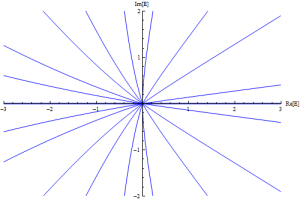
Figure 3: Some quantized complex energies $E$ for the potential $V(x)=x^{4}-5x^{2}$ for $-3<{\rm Re}\,E<3$ and $-2<{\rm Im}\,E<2$ [see (14)]. These curves represent some of the (infinite number of) special complex energies $E$ for which the classical orbits are periodic. These energies occur for rational values of $n/m\geq 2$. When $n=2$ and $m=1$, $E$ is real and positive. (This corresponds to oscillatory particle motion above the barrier in the potential.) The energy curve just above the positive-real axis in this figure corresponds to $(n,m)=(5,2)$. Subsequent energy curves in anticlockwise order correspond to $(n,m)=(3,1)$, $(n,m)=(4,1)$, $(n,m)=(5,1)$, $(n,m)=(7,1)$, $(n,m)=(10,1)$, $(n,m)=(20,1)$, $(n,m)=(40,1)$, and the negative real axis corresponds to $n/m=\infty$. (When $E<0$, the particle motion is oscillatory and confined to either the left or the right well.) The energy curves in the lower-half $E$ plane are complex conjugates of the energy curves in the upper-half $E$ plane. Near the origin these curves are asymptotically straight lines [see (15 and (16)].

Let us examine (14) for small $|E|$ and ${\rm Im}\,E>0$. When $|E|<<1$, $k^{2}\sim-\frac{2}{25}E$ and $k^{\prime}\sim 1+E/25$. Thus, using the asymptotic behaviors $K(\epsilon)\sim\textstyle{\frac{1}{2}}\pi$ ($\epsilon\to 0$) and $K(1-\epsilon)\sim\log(4/\sqrt{\epsilon})$ ($\epsilon\to 0$), we see that when $0\leq{\rm arg}\,E\leq\pi$, (14) reduces to

$${\rm arg}\,E\sim\pi\left(1-\frac{2m}{n}\right)\quad(|E|\to 0).$$ (15)

In this formula $m$ and $n$ are integers with $n\geq 2m$. When $-\pi\leq{\rm arg}\,E\leq 0$, the corresponding formula is

$${\rm arg}\,E\sim-\pi\left(1-\frac{2m}{n}\right)\quad(|E|\to 0).$$ (16)

Equations (15) and (16) show that the curves (see Fig. 3) for which the particle trajectories $x(t)$ are periodic emanate from $E=0$ as straight lines before they begin to curve.

Some periodic orbits corresponding to the quantized energies are shown in Figs. 4 – 7. All curves for a given value of $n/m$ have the same topology. In Fig. 4 we display two periodic orbits corresponding to $(n,m)=(3,1)$. For these curves we choose at random a complex energy $E=0.672\,543\,108\,9+i$ that lies on the $(3,1)$ curve in Fig. 3. In Fig. 5 we take $(n,m)=(5,2)$ and choose the energy to be $E=1.540\,288\,094\,6+i$. In Fig. 6 we take $(n,m)=(8,1)$ and choose $E=-0.852\,958\,824\,6+i$. In Fig. 7 we take $(n,m)=(14,3)$ and choose $E=-0.144\,984\,595\,5+i$.

Figure 4: Two periodic orbits for the quartic potential $V(x)=x^{4}-5x^{2}$ corresponding to $(n,m)=(3,1)$. We choose at random the complex energy $E=0.672\,543\,108\,9+i$, which lies on the $(3,1)$ curve in Fig. 3. One orbit (blue) oscillates between a pair of turning points (turning points are indicated by dots) and the other orbit (green) encloses the pair of turning points. Because of Cauchy’s theorem all orbits having the same energy have the same period.

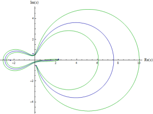
Figure 5: Two periodic orbits for the potential $x^{4}-5x^{2}$ for the case $(n,m)=(5,2)$. The energy is $E=1.540\,288\,094\,6+i$.

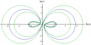
Figure 6: Two periodic orbits for $V(x)=x^{4}-5x^{2}$ for the case $(n,m)=(8,1)$. The energy is $E=-0.852\,958\,824\,6+i$.

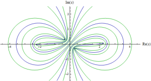
Figure 7: Two periodic orbits for $V(x)=x^{4}-5x^{2}$ for the case $(n,m)=(14,3)$. The energy is $E=-0.144\,984\,595\,5+i$.

Figures 4 – 7 illustrate an easy way to determine the ratio $n/m$ by examining the shape of the orbits: First, one determines $m$ by counting the number of times that the periodic orbit crosses the imaginary axis. Then one determines $n$ by counting the number of times that the orbit crosses two vertical lines, one between the left pair of turning points, and the other between the right pair of turning points. For example, in Fig. 4 the blue orbit crosses the imaginary axis once, so $m=1$, and it crosses a vertical line between the left pair of turning points twice and a vertical line between the right pair of turning points once, so $n=3$. Thus, the ratio $n/m=3$. For the green orbit we get $m=2$ and $n=6$, so again we find that $n/m=3$.

Similarly, in Fig. 5 for the blue orbit we count $m=2$ and $n=5$ and for the green orbit we count $m=4$ and $n=10$. Thus, $n/m=5/2$. In Figs. 6 and 7 it is easy to determine by inspection that $n/m=8$ and $n/m=14/3$.

IV Sextic and Octic Potentials

Higher degree polynomial potentials are significantly more complicated than quartic polynomial potentials because the classical trajectories are not elliptic functions. Thus, it is very difficult to study such potentials analytically. We have examined the complex trajectories of such potentials numerically, and we have found that there are still special quantized complex energy eigencurves for which the trajectories are periodic. However, the remarkable feature of polynomial potentials having degree higher than four is that now the behavior of trajectories depends on the initial condition. We find that there is a separatrix in the complex-coordinate plane that divides the periodic orbits from the nonperiodic paths. For example, in Fig. 8, which displays some trajectories for the sextic potential

$$V(x)=x^{6}-5x^{5}-4x^{4}+11x^{3}-\textstyle{\frac{11}{4}}x^{2}-13x,$$ (17)

we have plotted four trajectories for the energy $E=-4.359\,375+i$. There are three periodic orbits, one passing through $x=0$ (blue), a second passing through $x=i$ (cyan), and a third passing through $x=3i$ (green). However, there is a nonperiodic trajectory that begins at $x=5i$; this trajectory (red) spirals inward in an anticlockwise direction around the pair of turning points that lie just above and just below the positive real axis. Eventually this trajectory will cross the midline joining these two turning points and will then spiral outward. The nonperiodic trajectories are separated from the periodic trajectories by a separatrix curve that crosses the imaginary axis near $4i$ (not shown).

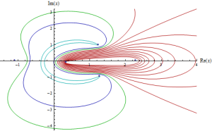
Figure 8: Periodic and nonperiodic trajectories for the sextic potential in (17). All trajectories correspond to the special complex energy $E=-4.359\,375+i$ and are either periodic or nonperiodic depending on the initial condition. The periodic orbits (blue, cyan, and green) are separated from the nonperiodic trajectories (red) by a separatrix curve (not shown).

In Fig. 9 we plot some trajectories for the octic potential

$$V(x)=(x-1)^{2}(x+1)^{2}(x-2)^{2}(x+2)^{2}$$ (18)

for the special complex energy $E=16.489+10i$. There are two periodic orbits, one starting at $x=0$ that oscillates between a pair of turning points (blue) and a second (cyan) that passes through $x=0.3$ and encircles these turning points. A nonperiodic trajectory (red) begins at $x=1$, spirals inward, then outward, and then inward. As time passes, this trajectory will continue to spiral outward and inward without ever crossing itself. The periodic and nonperiodic trajectories are separated by a separatrix curve (green). One part of the separatrix curve is shown passing through $x=0.670$ and the other part is shown passing through $x=i$. These two curves join in the upper-right quadrant and in the lower left quadrant.

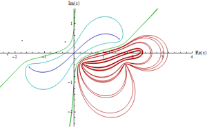
Figure 9: Periodic and nonperiodic trajectories for the octic potential in (18) for the energy $E=16.489+10i$. Two periodic trajectories (blue and cyan) and a nonperiodic trajectory (red) is shown. Two separatrix curves (green) separate the periodic trajectories from the nonperiodic trajectories. Numerical calculations suggest that the two separatrix curves meet at infinity in the first and third quadrants.

V Conclusions and Brief Remarks

We have shown in this paper that complex classical mechanics is richer and more elaborate than previously imagined. While it is generally true that a classical particle having complex energy traces an open trajectory, there are special discrete quantized curves in the complex-energy plane for which the classical particle has a periodic orbit.

For polynomial potentials the situation becomes more complicated as the degree of the polynomial increases: For quartic potentials (which, according to the lore of Riemann surfaces, are associated with the topology of a sphere) the orbits are always periodic, regardless of whether the energy is real or complex. For quadratic potentials (which are associated with the topology of a torus) the trajectories are open except for a discrete set of eigencurves in the complex-energy plane. When the energy lies on an eigencurve, the trajectory is always periodic regardless of the initial condition. For sextic and octic potentials (which are associated with the topology of a double and triple torus) there are eigencurves for which, depending on the initial condition, the particle trajectory may or may not be periodic. The periodic trajectories are separated from the nonperiodic trajectories by a separatrix curve.

The behavior of complex classical trajectories is analogous to the behavior of a quantum particle in a potential well. Ordinarily, a complex-energy classical particle in a double well potential follows a space-filling spiral trajectory as it alternately visits the left and the right well. However, we have shown in this paper that there is a discrete set of complex energy eigencurves for which the particle trajectories are periodic. The quantum analog is evident: The initial wave function of a quantum particle in a double-well potential spreads and diffuses as the particle tunnels from well to well. However, if the particle is initially in an eigenstate, the wave function remains stationary and merely oscillates in time.

One of our future objectives is to examine the nature of complex-energy classical trajectories in periodic potentials. In the case of quartic potentials one can make analytical progress because one can solve the equations of motion in terms of elliptic functions. This is not in general possible for sextic and higher-degree polynomial potentials. However, for periodic potentials such as $V(x)=\sin x$, one can again solve the the equations of motion in terms of elliptic functions. The behavior of complex trajectories in such potentials is surprising, and we expect to complete a paper on this subject soon R2 .

- (1) C. M. Bender, D. C. Brody, and D. W. Hook, J. Phys. A: Math. Theor. 41, 352003 (2008).
- (2) In early numerical studies of a complex-energy classical particle in a periodic potential two types of classical behavior were observed: For most complex energies the classical particle executes a deterministic random walk as it travels from well to well. In addition there appeared to be narrow conduction bands having sharp edges in the complex-energy plane, and for energies in these bands the classical particle appeared to drift from well to well in one direction only. See C. M. Bender and T. Arpornthip, Pramana J. Phys. 73, 259 (2009). In fact, the situation is more complicated than this: At discrete isolated energies in the conduction band there are special translationally invariant periodic solutions. Other solutions eventually turn around after a very long time. A paper on this remarkable complex behavior will be submitted shortly.
- (3) C. M. Bender, D. D. Holm, and D. W. Hook, J. Phys. A: Math. Theor. 40, F793-F804 (2007).
- (4) The harmonic oscillator is a glaring (and probably unique) example of a classical dynamical system that has closed orbits even when the classical energy is complex. When the classical energy is real, the classical orbits are all ellipses whose axes are parallel to the real and the imaginary axes, and as the energy becomes complex, the orientation of the ellipses changes.
- (5) C. M. Bender, Contemp. Phys. 46, 277 (2005) and Repts. Prog. Phys. 70, 947 (2007).
- (6) P. Dorey, C. Dunning, and R. Tateo, J. Phys. A: Math. Gen. 40, R205 (2007).
- (7) Experimental observations of the phase transition using optical wave guides are reported in A. Guo, G. J. Salamo, D. Duchesne, R. Morandotti, M. Volatier-Ravat, V. Aimez, G. A. Siviloglou, and D. N. Christodoulides, Phys. Rev. Lett. 103, 093902 (2009); C. E. Rüter, K. G. Makris, R. El-Ganainy, D. N. Christodoulides, M. Segev, D. Kip, Nature Phys. 6, 192 (2010). See also T. Kottos, Nature Phys. 6, 166 (2010).
- (8) Experimental observation of -symmetric diffusion of spin-polarized rubidium atoms is reported in K. F. Zhao, M. Schaden, and Z. Wu, Phys. Rev. A 81, 042903 (2010).
- (9) C. M. Bender, S. Boettcher, and P. N. Meisinger, J. Math. Phys. 40, 2201 (1999).
- (10) A. Nanayakkara, Czech. J. Phys. 54, 101 (2004) and J. Phys. A: Math. Gen. 37, 4321 (2004).
- (11) F. Calogero, D. Gomez-Ullate, P. M. Santini, and M. Sommacal, J. Phys. A: Math. Gen. 38, 8873-8896 (2005).
- (12) C. M. Bender, J.-H. Chen, D. W. Darg, and K. A. Milton, J. Phys. A: Math. Gen. 39, 4219 (2006).
- (13) C. M. Bender and D. W. Darg, J. Math. Phys. 48, 042703 (2007).
- (14) C. M. Bender and D. W. Hook, J. Phys. A: Math. Theor. 41, 244005 (2008).
- (15) Yu. Fedorov and D. Gomez-Ullate, Physica D 227, 120 (2007).
- (16) C. M. Bender, D. C. Brody, J.-H. Chen, and E. Furlan, J. Phys. A: Math. Theor. 40, F153 (2007).
- (17) A. Fring, J. Phys. A: Math. Theor. 40, 4215 (2007).
- (18) B. Bagchi and A. Fring, J. Phys. A: Math. Theor. 41, 392004 (2008).
- (19) C. M. Bender and J. Feinberg, J. Phys. A: Math. Theor. 41, 244004 (2008).
- (20) T. L. Curtright and D. B. Fairlie, J. Phys. A: Math. Theor. 41 No 24 (20 June 2008) 244009 (2pp)
- (21) C. M. Bender, F. Cooper, A. Khare, B. Mihaila, and A. Saxena, Pramana J. Phys. 73, 375 (2009).
- (22) P. E. G. Assis and A. Fring, arXiv:0901.1267.
- (23) C. M. Bender, J. Feinberg, D. W. Hook, and D. J. Weir, Pramana J. Phys. 73, 453 (2009).
- (24) A. V. Smilga, J. Phys. A: Math. Theor. 42, 095301 (2009).
- (25) A. Mostafazadeh, Phys. Rev. Lett. 102, 220402 (2009).
- (26) C. M. Bender, D. W. Hook, P. N. Meisinger, and Q. Wang, Phys. Rev. Lett. 104, 061601 (2010) and Ann. Phys. 325, 2332-2362 (2010).
- (27) Z. Ahmed, C. M. Bender, and M. V. Berry, J. Phys. A: Math. Gen. 38, L627 (2005).