A graphical theory of competition on spatial resource gradients

Abstract

Resource competition is a fundamental interaction in natural communities. However little is known about competition in spatial environments where organisms are able to regulate resource distributions. Here, we analyze the competition of two consumers for two resources in a one-dimensional habitat in which the resources are supplied from opposite sides. We show that the success of an invading species crucially depends on the slope of the resource gradients shaped by the resident. Our analysis reveals that parameter combinations which lead to coexistence in a uniform environment may favor alternative stable states in a spatial system, and vice versa. Furthermore, differences in growth rate, mortality or dispersal abilities allow a consumer to coexist stationarily with - or even outcompete - a competitor with lower resource requirements. Applying our theory to a phytoplankton model, we explain shifts in the community structure that are induced by environmental changes.

Keywords: competition, coexistence, limiting resources, spatial system, meta-ecosystem, invasion analysis

Correspondence email: a.ryabov@icbm.de, blasius@icbm.de

Ecology Letters (2011) 14: 220–228

INTRODUCTION

Competition for limiting resources is one of the most important species interactions in ecology and has long been considered as a major driver for shaping the spatial structure of communities and limiting species richness. A graphical theory of resource competition was advanced by MacArthur (1972), León & Tumpson (1975) and Tilman (1980, 1982) and revolves around the assumption that consumers that reduce limiting resources to the lowest level will exclude all other competitors (the $R^{*}$-rule). Being confirmed experimentally (Miller et al. 2005, but see also Wilson et al. 2007), this theory provides a fundamental framework for interpreting the relationship between organisms and their shared resources in a uniform environment (Grover 1997; Chase & Leibold 2003). Extensions of competition theory to spatial settings (Chesson 2000a, 2000b; Klausmeier & Tilman 2002; Amarasekare 2003) can be grouped into different classes. In spatially homogeneous environments, coexistence can be mediated by trade-offs in life history parameters (Levins & Culver 1971; Levin 1974; Kneitel & Chase 2004). In heterogeneous environments regional coexistence can be mediated by spatial segregation (Tilman 1982; Gross and Cardinale 2007), whereas local coexistence may be promoted via source-sink effects (Mouquet & Loreau 2003; Leibold et al. 2004) or positive correlations between dispersal and competitive abilities (Abrams & Wilson 2004). However, previous theory has not thoroughly explored resource competition in continuous spatially variable habitats.

In a system with resource flows, spatial heterogeneity can be created by biotic interactions, as local resource consumption can modify resource levels over larger ranges (Huston & DeAngelis 1994), possibly establishing resource gradients over the full extent of the habitat. The analysis of competition in such systems is mathematically challenging (Grover 1997), as not only the resource availability, but also the size of favorable areas (Skellam 1951), dispersal rates (Abrams & Wilson 2004) and many other factors become crucial for the survival of a population (Ryabov & Blasius 2008). Despite extensive theoretical studies on unstirred chemostats (Hsu & Waltman 1993; Smith & Waltman 1995; Wu et al. 2004), persistence and competition in streams (Speirs & Gurney 2001; Lutscher et al. 2007), vegetation patterns in water-limited habitats (Klausmeier 1999; von Hardenberg et al. 2001), well-mixed systems with a light gradient (Huisman & Weissing 1994; Diehl 2002), and non-uniform phytoplankton systems (Dutkiewicz et al. 2009; Yoshiyama et al. 2009; Ryabov et al. 2010), translating competition theory to extended systems, where species are able to shape resource distributions, still remains a great challenge.

In this study we develop a general framework for analyzing the competition between two consumers for two limiting resources in a spatially continuous habitat in which resource distributions are regulated by biotic interactions. In extension of the $R^{*}$-rule for uniform systems, we introduce the notion of an invasion threshold in a spatial system as the maximal resource requirement for a consumer to invade in the presence of a resident species. In this way, the outcome of competition can be interpreted graphically in the resource plane, by comparing the location of the invader’s critical resources with respect to the invasion threshold lines. We derive analytic expressions for the invasibility conditions and show that they can be related to how resources are spatially reduced as a result of resource-use by the resident.

Using this approach we find that environmental heterogeneity increases the likelihood of coexistence. Thereby we identify two forms of stationary coexistence in spatially variable habitats. First, coexistence can be mediated by a trade-off in resource requirements. This is characterized by spatial segregation of the two species and we find that parameter combinations which allow coexistence in a uniform system favor alternative stable states in a spatially extended system and vice versa. Second, coexistence can arise from positive correlations of growth rates and resource requirements (gleaner-opportunist trade-off), characterized by a lack of spatial segregation.

To illustrate these ideas, we investigate two phytoplankton species competing for light and a nutrient in a water column. We identify two distinct regimes of bistability in the competition outcome and show that our approach provides a powerful basis for projecting the influence of environmental changes on the community composition.

MODELLING FRAMEWORK AND ANALYSIS

Resource competition in uniform systems

As a background for the following discussion, we briefly review the theory of resource competition in a uniform environment (MacArthur 1972; León and Tumpson 1975; Tilman 1980, 1982; Grover 1997; Chase & Leibold 2003). Consider two consumer species $i=1,2$ growing on two essential resources $N$ and $I$. The dynamics of the population density $P_{i}$ of each species is determined by the difference between growth $\mu_{i}(N,I)$ and mortality $m_{i}$

$$\dot{P}_{i}=(\mu_{i}(N,I)-m_{i})\,P_{i}\,,$$ (1)

where the growth rate in general can be written as

$$\mu_{i}(N,I)=\mu_{max,i}\,\,\mu\left(\frac{N}{H_{N,i}},\frac{I}{H_{I,i}}\right).$$ (2)

Here $\mu_{max,i}$ is the maximal growth rate of species $i$, $\mu$ is a monotonically increasing function of both arguments with upper bound $\lim_{N,I\rightarrow\infty}\mu(N,I)=1$, and the half-saturation constants $H_{N,i}$ and $H_{I,i}$ define the species’ resource adaptation. In particular, this functional form includes von Liebig’s law of minimum, where the limitation of growth follows the Monod kinetics

$$\mu_{i}(N,I)=\mu_{max,i}\,\,\min\left\{\frac{N}{N+H_{N,i}}\ ,\ \frac{I}{I+H_{I,i}}\right\}\ .$$ (3)

In a uniform environment, levels of system resources can be represented as a point in a two-dimensional resource plane (Fig. 1a). In this plane, states of balance between growth and mortality, $\mu_{i}(N,I)=m_{i}$, determine the zero net growth isoclines (ZNGIs), which for each species divide the resource plane into areas of positive and negative population net growth. Assuming eqn 3 for the growth rate, we can calculate the critical values, $I^{*}_{i}=H_{I,i}\ m_{i}/(\mu_{max,i}-m_{i})$ and $N^{*}_{i}=H_{N,i}\ m_{i}/(\mu_{max,i}-m_{i})$, and the ZNGI takes the form of two orthogonal lines (dashed lines in Fig. 1).

The resource concentrations in the absence of consumers define the coordinates of a resource supply point $S$. A growing population will deplete resources, shifting the system state in the direction of the consumption vector $CV$, until the system state point hits the population’s ZNGI at the equilibrium point $E=(\widetilde{N}_{i},\widetilde{I}_{i})$. This point defines the resource levels at equilibrium, which are shaped by the population, and sets the conditions for the invasion of other species.

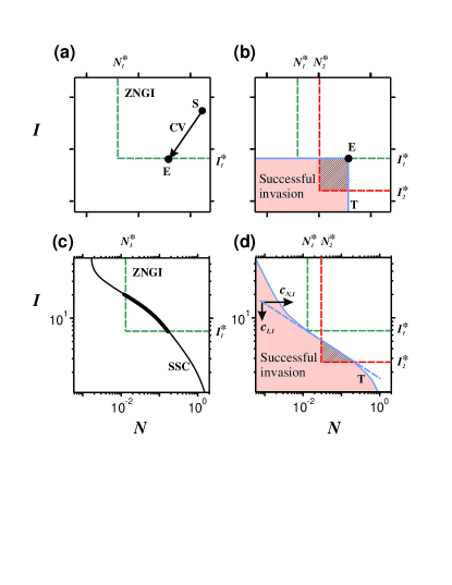
Figure 1: Invasion analysis in a uniform system (top) and a spatially extended system with opposing resource gradients (bottom). (a) Equilibrium configuration of the resident (species 1, green). The system state point at equilibrium $E$ is determined by the intersection of the consumption vector $CV$, starting at the resource supply point $S$, with the zero net growth isocline ZNGI (dashed line, see text). (b) Critical resource values of a successful invader (species 2, red) should be located below the invasion threshold $T$ (blue line). The intersection of the invader’s ZNGI with $T$ is shown as cross-hatching. (c) In a spatially extended system, combinations of resources at different spatial coordinates give rise to a system state curve SSC (solid line, favorable range is marked in bold). (d) Invasion threshold $T$ (blue solid line) and first order approximation (blue dashed line) with slope $\gamma_{1}=c_{I,1}/c_{N,1}$ in the log-log plot (eqn 12). (c) and (d) show results of numerical simulations in the phytoplankton model, eqns 3–6 (see Appendix S5 for model parameters).

Assume that resident species 1 has attained equilibrium. Then invasion of a second species 2 is possible if the equilibrium resource concentrations shaped by the resident are sufficient to allow positive growth of the invader. Thus, in resource space a part of the invader’s ZNGI must be located below the equilibrium point $E$ (Fig. 1b). For the specific form of eqn 3, this condition is fulfilled for all critical resource values of the invader that are located in the rectangular area defined by $I^{*}_{2}<\widetilde{I}_{1}$ and $N^{*}_{2}<\widetilde{N}_{1}$. This line defines the invasion threshold $T$ for species 2 (blue line in Fig. 1b).

Combining the invasion analysis for each of the two species yields the well-known outcomes of resource competition in a uniform environment (Tilman 1982). Without a trade-off in the use of the two resources (i.e. the two ZNGIs do not intersect), the species with the lowest resource requirements wins. In the presence of a trade-off, competition can lead to stable coexistence, competitive exclusion or bistability (i.e. alternative stable states with outcomes depending on initial conditions), depending on whether or not each species has a greater impact on the resource that most limits its own growth (see Fig. S1).

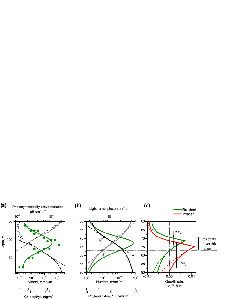
Figure 2: Typical distributions of light (gray), nutrient (black) and chlorophyll/phytoplankton (green) concentrations in a water column from (a) field measurements (HOT program, Station ALOHA, cruise 114; see also Karl 2010) and (b) numerical simulation of eqns 3–6. Dashed lines in (a) and (b) indicate exponential fit of the resource distributions. (c) Net growth rates, $\mu_{i}(N,I)-m$, of a resident (species 1, green) and an invader (species 2, red), derived from the simulated distribution of resources (solid lines) and from their exponential approximation (eqn 7, dashed lines). Horizontal dashed lines in (b) and (c) mark the favorable range of species 1. Vertical shifts $\Delta z_{N}$ and $\Delta z_{I}$, related to nutrient and light limitation (eqn 10), are also shown. Model parameters as in Fig. 1.

Resource distributions in a spatial system

The classical approach implicitly assumes the presence of boundaries which confine the system, between which organisms and resources are uniformly distributed. In the following we aim to translate these ideas to an open system where the favorable area of a species is confined by resource availability, and where organisms and resources are not distributed uniformly. Consider a one-dimensional environment, where the population densities $P_{i}(z,t)$ depend on a spatial coordinate $z$. A spatial analog to eqn 1 can be written in the form

$$\frac{\partial P_{i}}{\partial t}=(\mu_{i}(N,I)-m_{i})\,P_{i}+D_{i}\frac{\partial^{2}P_{i}}{\partial z^{2}}\ ,\\$$ (4)

where $D_{i}$ characterizes the diffusive dispersal ability of population $i$. Again the growth rate $\mu_{i}(N,I)$ follows the general form of eqn 2, but the resource concentrations $N(z,t)$ and $I(z,t)$ are functions of $z$, so that the two populations are indirectly coupled through the spatial profile of their shared resources.

As a case study, we examine a two-species phytoplankton-nutrient model in an incompletely mixed water column (Radach & Maier-Reimer 1975, Jamart et al. 1977, Klausmeier & Litchman 2001, Huisman et al. 2006, Ryabov et al. 2010). In the model, eqn 4 describes the density $P_{i}(z,t)$ of phytoplankton species $i$ at depth $z$ and time $t$, and is complemented by an equation for the nutrient $N(z,t)$

$$\frac{\partial N}{\partial t}=-\sum_{i=1}^{n}\alpha_{i}\mu_{i}(N,I)P_{i}+D\frac{\partial^{2}N}{\partial z^{2}}\ ,$$ (5)

and an equation for the light intensity $I(z,t)$, which describes the absorption of light by water and phytoplankton (Kirk 1994)

$$I(z)=I_{in}\exp\left[-K_{bg}z-\int^{z}_{0}\sum_{i=1}^{n}k_{i}P_{i}(\xi,t)d\xi\right]\ .$$ (6)

In these equations, parameter $D$ obtains the role of the turbulent diffusivity, $\alpha_{i}$ is the nutrient content of a phytoplankton cell, $I_{in}$ is the incident light intensity, $K_{bg}$ is the water turbidity and $k_{i}$ is the attenuation coefficient of phytoplankton cells. As boundary conditions we assumed impenetrable borders at the surface and at the bottom for the phytoplankton biomass and an impenetrable surface and a constant concentration $N_{B}$ at the bottom for the nutrient (for model parameters see Table S1).

The model describes a situation in which the two resources, light and nutrient, are supplied from opposite sides of a spatial habitat. This is typical in the ocean where light is supplied from above and many macronutrients from below (Fig. 2a). As shown in Fig. 2b, this gives rise to characteristic resource distributions with inverse gradients, where population growth is maximal at an intermediate position at which both resources are sufficiently available (see Fig. S6 for further typical model solutions).

Within the favorable range of the population, the light and nutrient distributions in Figs. 2a and 2b can be well approximated as straight lines on a logarithmic scale. This means that resource distributions at equilibrium decay (or grow) exponentially in space

$$\widetilde{N}_{i}(z)\sim e^{c_{N,i}\,z},\ \ \widetilde{I}_{i}(z)\sim e^{-c_{I,i}\,z}\,.$$ (7)

This exponential dependence can be derived analytically in the limit of low mortality (see Appendix S1), and it is typical for many other ecosystems (see e.g. Fig. S5). Eqn 7 implies that a population $i$ in monoculture is “shading” resources by a constant percentage

$$c_{N,i}=\frac{1}{N_{i}}\frac{dN_{i}(z)}{dz},\quad c_{I,i}=-\frac{1}{I_{i}}\frac{dI_{i}(z)}{dz}\ .$$ (8)

Here, the logarithmic resource gradients $c_{N,i}$ and $c_{I,i}$ measure the influence of the population on the resource distribution.

Translated into the resource plane, the resource distributions of the spatially extended system can be compactly represented as a parametric curve, $(N(z),I(z))$, (solid line in Fig. 1c). This ‘system state curve’ (SSC) naturally extends the notion of a system state point E of a homogeneous system to a spatially continuous environment (Ryabov et al. 2010). As shown in Fig. 1c, due to the spatial coupling and source-sink effects the system state curve at equilibrium does not settle at the ZNGI. Instead, it intersects the ZNGI at two points which mark the boundaries of positive net growth. This inner part of the system state curve (marked in bold in Fig. 1c) corresponds to the resident’s favorable range (horizontally dashed lines in Fig. 2b, c). Given the exponential dependence (eqn 7), within the favorable range the system state curve approaches a straight line with slope $\gamma_{i}=c_{I,i}/c_{N,i}$ in the resource plane with logarithmic axes (see Fig. 1c in the model or Fig. S4c for field data).

Invasion analysis in a spatial system

In analogy to competition theory in a uniform system, we may now ask whether it is possible to predict the outcome of two-species competition from knowledge about equilibrium resource distribution which has been shaped by each species alone in the absence of the other species. Assuming that we know the resident’s system state curve at equilibrium $(\widetilde{N}_{1}(z),\widetilde{I}_{1}(z))$, what can we say about the success of an invader (red color in Fig. 2c)?

To address this problem we define the invasion threshold T in the resource plane as the set of critical resources of all invaders of small initial density, which have zero total growth in the presence of the resident (blue solid line in Fig. 1d, obtained by invasion analysis in numerical simulations with 7000 parameter combinations). In this formulation, the success of an invader depends on whether or not its ZNGI intersects with the invasion threshold (cross-hatching in Fig. 1). Thus, invasion analysis can be performed graphically by comparing the location of the invader’s critical resources with the invasion threshold.

By comparison of Figs. 1b and 1d, the invasion threshold has a different shape in a uniform or a spatially continuous system. It is difficult to predict the invasion threshold from general principles. Exact conditions can be expressed in terms of eigenvalues of a corresponding boundary value problem (Hsu & Waltman 1993; Appendix S3), which unfortunately cannot be solved in general. In the following we show that, with the assumption of exponential resource distributions (eqn 7), it is possible to calculate the invasion threshold for species with similar resource requirements.

Calculation of the invasion threshold

Consider first the simplest case where resident (species 1) and invader (species 2) differ only in their half saturation constants, $H_{N,i}$ and $H_{I,i}$, but are otherwise identical ($\mu_{max,1}=\mu_{max,2}$, $m_{1}=m_{2}$, $D_{1}=D_{2}$). As the invader density is assumed to be small, and its influence on the resource distributions can thus be neglected, the possibility of invasion depends entirely on the invader’s growth rate in the equilibrium resource distribution shaped by the resident, $\mu_{2}(\widetilde{N}_{1}(z),\widetilde{I}_{1}(z))$. The mathematical identity

$$\frac{1}{H_{2}}e^{cz}=\frac{1}{H_{1}}e^{c(z-\Delta z)}\ ,\quad\mbox{with}\ \Delta z=\frac{1}{c}\ln\frac{H_{2}}{H_{1}}\ ,$$ (9)

shows that division of an exponential function by different (half-saturation) constants $H_{1}$ and $H_{2}$ is equivalent to a shift $\Delta z$ in position along the $z$-axis. Therefore, assuming that the growth rate follows eqn 2 and the resource distributions are exponential (eqn 7), it is possible to express the growth rate, $\mu_{2}(z)$, of the invader through that of the resident

$$\mu_{2}(\widetilde{N}_{1}(z),\widetilde{I}_{1}(z))=\mu_{1}(\widetilde{N}_{1}(z-\Delta z_{N}),\widetilde{I}_{1}(z-\Delta z_{I}))\ .$$ (10)

Here the shifts $\Delta z_{N}=c_{N,1}^{-1}\ln H_{N,2}/H_{N,1}$ and $\Delta z_{I}=-c_{I,1}^{-1}\ln H_{I,2}/H_{I,1}$ have opposite signs, since the resource gradients are inverse.

Introducing a new position $z^{\prime}=z-\Delta z_{N}$, we find that $\mu_{2}(z)=\mu_{1}(\widetilde{N}_{1}(z^{\prime}),\widetilde{I}_{1}(z^{\prime}+\Delta)),$ with $\Delta=\Delta z_{N}-\Delta z_{I}$. The change of variables $z\rightarrow z^{\prime}$ corresponds to a shift along the z-axis (see Fig. 2c) and has no effect on the conditions for survival as long as boundary effects can be neglected. Thus, the difference in growth between invader and resident depends only on the value and sign of the single parameter $\Delta$. If $\Delta=0$, the distinct resource requirements of the species just result in a parallel translation of the growth rate profile. Since the resident species at equilibrium has zero total growth, the same holds for the invader, and the population of the invader cannot establish. By contrast, if $\Delta>0$, we obtain $I(z^{\prime}+\Delta)<I(z^{\prime})$ since $I(z)$ decays with $z$. This leads to negative net growth of the invader since the function $\mu(N,I)$ increases monotonically with its arguments. Using the same arguments, $\Delta<0$ gives rise to positive growth of the invader.

Thus, we can formulate the invasibility criterion in the form $\Delta<0$. The parameter $\Delta$ describes the invasion threshold and can be interpreted in terms of resource gradients and relative competitive abilities

$$\Delta\,\,=\underbrace{\frac{1}{c_{N,1}}}_{\begin{smallmatrix}\text{inverse}\\ \text{log gradient}\\ \text{in $N$}\end{smallmatrix}}\underbrace{\ln\frac{H_{N,2}}{H_{N,1}}}_{\begin{smallmatrix}\text{log of relative }\\ \text{competitive}\\ \text{abilities for $N$}\end{smallmatrix}}+\underbrace{\frac{1}{c_{I,1}}}_{\begin{smallmatrix}\text{inverse}\\ \text{log gradient}\\ \text{in $I$}\end{smallmatrix}}\underbrace{\ln\frac{H_{I,2}}{H_{I,1}}}_{\begin{smallmatrix}\text{log of relative }\\ \text{competitive}\\ \text{abilities for $I$}\end{smallmatrix}}\,.$$ (11)

If for instance, both species have equal resource requirements for $N$, $H_{N,2}=H_{N,1}$, invasion is only possible, $\Delta<0$, if the invading species is a better competitor for $I$, i.e. $\ln(H_{I,2}/H_{I,1})<0$.

If the limitation of growth follows von Liebig’s law (eqn 3), the spatial profiles for light and nutrient limitation are shifted independently and the net shift $\Delta=\Delta z_{N}-\Delta z_{I}$ measures the difference in the size of the resident and invader’s favorable habitats. This is depicted in Fig. 2c for a situation with $\Delta z_{N}<\Delta z_{I}$, where the narrowing of the favorable range due to higher $N$ requirements ($N_{2}^{*}>N_{1}^{*}$) is less than the widening due to better $I$ adaptation ($I_{2}^{*}<I_{1}^{*}$). Therefore the net growth rate of the invader is greater than that of the resident, allowing for successful invasion (see Fig. 2c). Note that in the example shown in Figs. 1 and 2, the invader, species 2, is a good light competitor, $I^{*}_{2}<I^{*}_{1}$, but needs higher nutrient concentrations, $N^{*}_{2}>N^{*}_{1}$. Therefore it will have maximal production at a deeper depth (Fig. 2c).

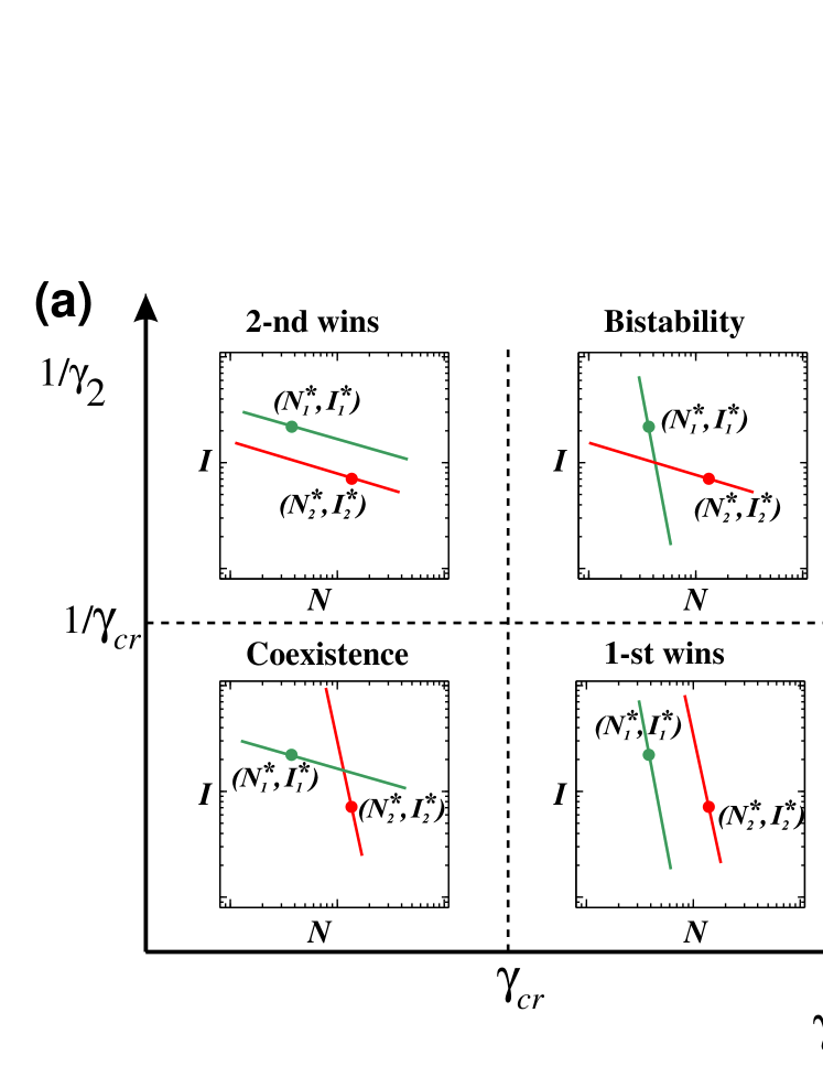
Figure 3: The four different cases of spatial resource competition depending on the ratio $\gamma_{i}$ of logarithmic resource gradients: ($\gamma_{1}<\gamma_{cr}$, $1/\gamma_{2}<1/\gamma_{cr}$) coexistence; ($\gamma_{1}>\gamma_{cr}$, $1/\gamma_{2}>1/\gamma_{cr}$) alternative stable states; ($\gamma_{1}>\gamma_{cr}$, $1/\gamma_{2}<1/\gamma_{cr}$) species 1 wins; ($\gamma_{1}<\gamma_{cr}$, $1/\gamma_{2}>1/\gamma_{cr}$) species 2 wins. (a) Schematic representation. Insets sketch invasion threshold lines for resident species 1 (green) and invader species 2 (red), and critical resource values (dots) in the resource plane. (b) Numerical verification in the phytoplankton model, based on more than 1000 simulations, with parameter values randomly chosen from a wide range (critical resources $(N_{i}^{*},\ I_{i}^{*}$) and $\gamma_{cr}$ remain constant, see Appendix S5). The color scale shows the logarithm of relative species abundance $\ln B_{1}/B_{2}$ at equilibrium (total biomass $B_{i}=\int_{0}^{Z_{B}}P_{i}(z)\,dz$). Upward-pointing triangles indicate the simulation outcome when species 1 is the resident and species 2 the invader, downward-pointing triangles show the opposite case; their color is different only if the competition outcome is bistable.

Since the maximal growth and mortality rates are assumed to be equal for both species, the ratio of half-saturation constants equals the ratio of critical resource values (e.g., $H_{I,2}/H_{I,1}=I^{*}_{2}/I^{*}_{1}$), and the invasibility criterion reads

$$\Delta=\frac{1}{c_{N,1}}\ln\frac{N^{*}_{2}}{N^{*}_{1}}+\frac{1}{c_{I,1}}\ln\frac{I^{*}_{2}}{I^{*}_{1}}<0\ .$$ (12)

This expression has a straightforward geometrical interpretation: a species can invade the spatial habitat if its critical resources $(N^{*}_{2},\ I^{*}_{2})$ are located below a straight line, $\ln I-\ln I^{*}_{1}=-\gamma_{1}(\ln N-\ln N^{*}_{1})$, with a slope of absolute value $\gamma_{1}=c_{I,1}/c_{N,1}$ passing through the point $(N^{*}_{1},\ I^{*}_{1})$ in the double-logarithmic resource plane (blue dashed line in Fig. 1d). Thus, we have derived a first-order approximation for the invasion threshold T.

Competition outcome

In a similar way it is possible to analyze the invasion potential of species 1 in a system with resident species 2. Assume without loss of generality that $N^{*}_{2}>N^{*}_{1}$ and $I^{*}_{2}<I^{*}_{1}$, and denote by $\gamma_{cr}$ the slope (taken with opposite sign) of a straight line passing through the two critical resource points, $\gamma_{cr}=-(\ln I^{*}_{2}/I^{*}_{1})/(\ln N^{*}_{2}/N^{*}_{1})$. Then, combining eqn 12 and its counterpart for species 2, we obtain four different outcomes of spatial resource competition (Fig. 3a). If the critical resource values for each species are located below the invasion threshold of its competitor, $\gamma_{1}<\gamma_{cr}$ and $1/\gamma_{2}<1/\gamma_{cr}$, both species can invade the monoculture of the other, leading to coexistence. In the opposite case, if the critical resource values for every species lie above the invasion threshold of its competitor, $\gamma_{1}>\gamma_{cr}$ and $1/\gamma_{2}>1/\gamma_{cr}$, neither of the two species can invade, leading to bistability. Finally, one species may be a superior competitor if only this species can grow in the presence of its competitor.

This analytic conclusion is confirmed by numerical simulations of the phytoplankton model eqns 3-6 in a large parameter range (Fig. 3b). The figure demonstrates that in spite of the high complexity and nonlinearity of the model, the relation between the slope of the invasion threshold lines, $\gamma_{i}$, and the location of the critical resource values gives a good prediction of the competition outcome.

Differences in growth, mortality and dispersal

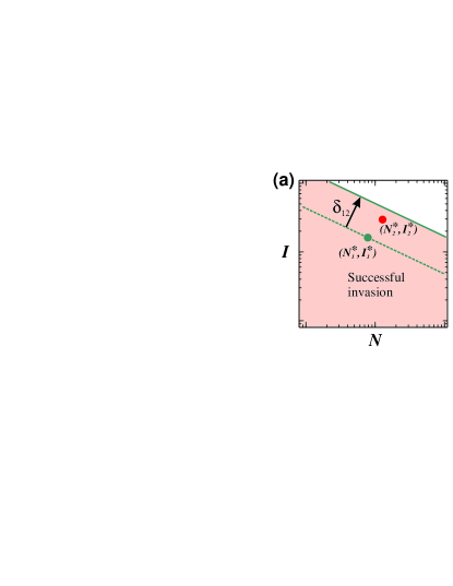
Figure 4: (a) Interspecific differences in $\mu_{max}$, $m$, or $D$ yield a shift $\delta_{12}$ of the invasion threshold in the normal direction. Compared with Fig. 1d, the invader (species 2, red) can establish, even though it has higher resource requirements than the resident (species 1, green). (b) Coexistence due to a gleaner-opportunist trade-off, where both invasion thresholds are shifted in opposite directions. Species 1 (gleaner) with lower resource requirements can coexist at equilibrium with species 2 (opportunist), which has higher resource requirements but higher $\mu_{max}$, or lower $m$ or $D$.

In general, the locations of the invasion thresholds may depend on trait differences between the resident and invader, such as maximal growth rate, mortality and dispersal rates. As shown in Appendix S3, the generalized form of the invasibility criterion reads

$$\frac{1}{c_{N,1}}\ln\frac{N^{*}_{2}}{N^{*}_{1}}+\frac{1}{c_{I,1}}\ln\frac{I^{*}_{2}}{I^{*}_{1}}<\Delta_{12}$$ (13)

where $\Delta_{12}$ is a complicated function of the trait values and resource gradients, but does not depend on the critical resource levels. If all trait differences vanish, we obtain $\Delta_{12}=0$ and recover the previous result, eqn 12. The geometrical representation of the new term $\Delta_{12}$ is a shift of the invasion threshold line toward larger ($\Delta_{12}>0$) or smaller ($\Delta_{12}<0$) resource requirements in the normal direction by $\delta_{12}=\Delta_{12}c_{N,1}c_{I,1}/\sqrt{c^{2}_{N,1}+c^{2}_{I,1}}$. Thus, the slope of the invasion threshold lines remain unchanged, but their location is shifted. Fig. 4a shows an example with a positive shift of the invasion threshold, where species 2 can invade the system despite the fact that it has higher requirements for both resources than the resident species 1.

For an illustration of how specific trait values can change the sign of $\delta_{12}$, consider the particular case that species 2 has higher values of both growth rate, $\mu_{max,2}=\beta\mu_{max,1}$, and mortality, $m_{2}=\beta m_{1}$, with $\beta>1$. Since the critical resource values $N^{*}_{2}>N^{*}_{1}$ and $I^{*}_{2}>I^{*}_{1}$ are independent of $\beta$, this scaling would not affect the competition outcome in a uniform environment and species 2 would not be able to invade the system. However, in a heterogeneous system the invasion threshold (green line in Fig. 4b) is shifted by $\delta_{12}>0$ (see Appendix S3). Similar analysis, using rescaling by a factor of $1/\beta$, shows that the threshold for invasion of species 1 in a monoculture of species 2 is shifted in the opposite direction (red line in Fig. 4b). This mechanism can lead to stable coexistence of a species having high growth rate and resource requirements with another species having low growth rate and resource requirements (gleaner-opportunist trade-off).

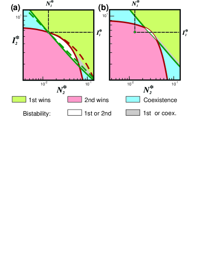
Figure 5: Competition analysis in the phytoplankton model. Maximal growth rates and mortalities are (a) identical, $\beta=1$, and (b) different, $\beta=2$. The competition outcome (in color coding) of species 1 (critical resource values indicated as circle) is shown in dependence of the critical resource values of species 2. Solid lines show invasion thresholds obtained from numerical simulation of eqns 3–6; dashed lines in (a) show their analytical approximations (Appendix S2). Parameter combinations $(N_{2}^{*},I_{2}^{*})$ in the area below the solid green line allow invasion of species 2 in the presence of species 1. In contrast, species 1 can invade in the presence of species 2 with critical resource values taken from the area above the solid red line. The intersections of these lines define the ranges of coexistence, alternative states, and competitive exclusion.

Application to a phytoplankton model

Applying this approach to a phytoplankton community, the slopes $\gamma_{i}$ of the invasion lines can be obtained by numerical simulations (Fig. S2), analytic estimations (Appendix S1), or in field enclosure experiments (Jäger et al. 2008). Tracing the dependence of $\gamma_{i}$ as a function of system parameters allows us to project shifts in the species composition. Consider, for instance, the effects of increasing the nutrient resource concentration at the bottom of the water column, $N_{B}$. More nutrients at the bottom give rise to a larger biomass of the resident species, which in turn yields a steeper nutrient decay within the production layer, i.e. a reduction of $\gamma_{i}$ (see Fig. S2c). In the resource plane this effectively leads to a counter-clockwise rotation of the invasion threshold line, and graphical analysis reveals that by increasing $N_{B}$ the community composition shifts from dominance of the best nutrient competitor, through a regime of coexistence, to the prevalence of the best light competitor (Fig. S3). This result might explain observed negative correlations of the abundance of high light-adapted species with nutrient concentrations (Johnson et al. 2006).

Similarly we can study the influence of consumption rates. In a well-mixed water column the slope of consumption vectors is given by $\Gamma_{i}=(k_{i}\,z_{B})/\alpha_{i}$ (Huisman & Weissing, 1994; Diehl 2002). Thus, the relative resource consumption scales with the ratio of the light attenuation coefficient to the cell nutrient content, $k_{i}/\alpha_{i}$. In our model, according to Fig. 3, two species coexist if $\gamma_{1}<\gamma_{cr}<\gamma_{2}$. Since the ratio of resource gradients $\gamma_{i}$ also grows with $k_{i}/\alpha_{i}$ (see Fig. S2a and eqn S6), we observe coexistence if the best nutrient competitor (here species 1) has a small $k_{1}/\alpha_{1}$ ratio and species 2 a large $k_{2}/\alpha_{2}$ ratio. The reverse situation (large $k_{1}/\alpha_{1}$ and small $k_{2}/\alpha_{2}$) leads to bistability (Fig. 3a). Thus, we obtain a rule which is diametrically opposed to that for uniform systems: coexistence arises if each species reduces its least limiting resource more strongly in relation to the other, whereas stronger reduction of the most limiting resource favors bistability (compare Figs. 3 and S1).

Fig. 5a shows the competition outcome in dependence of the critical resources of species 2 for the case that $k_{1}/\alpha_{1}>k_{2}/\alpha_{2}$, i.e. species 1 shades relatively more light than species 2. In accordance with our rule, if species 2, which has a smaller light attenuation coefficient, is more strongly limited by light ($I_{2}^{*}>I_{1}^{*}$), it may coexist with species 1 (upper blue area), whereas stronger nutrient limitation of species 2 ($N_{2}^{*}>N_{1}^{*}$) can lead to bistability (white area). However, if the difference in nutrient limitation is sufficiently large, then the two species can again coexist (lower blue area, Appendix S2). The model further exhibits a regime of bistability between coexistence and single-species dominance (gray area), where the invasion of species 1 does not exclude species 2, but species 2 cannot invade if species 1 has already established (see also the vertical profiles in Fig. S6). If the two species differ in their maximal growth and mortality rates, $\beta>1$ (Fig. 5b), all bifurcation lines are shifted towards larger critical resource values. Then, if species 2 is parameterized to have higher resource requirements (i.e., critial resource levels located above the black dashed lines in Fig. 5b), it can have all possible competition outcomes, even without a trade-off in resource requirements. The corresponding spatial profiles in Fig. S6 reveal two fundamentally different types of coexistence in a spatial system, mediated either by a trade-off in resource requirements (characterized by spatial segregation of the two species) or by a gleaner-opportunist trade-off (lack of spatial segregation).

	Uniform system	Spatial system with resource gradient
Invasion threshold	simple form defined by resource values,	curved shape, defined by gradients and resource availability,
	on the ZNGI	location depends on differences in $\mu_{max}$, $m$, or $D$
Coexistence with	each species mostly consumes	each species mostly consumes its least limiting resource or
resource trade-off	its most limiting resource	essential difference in resource requirements
		$\to$ spatial profiles with separation
Coexistence without	not possible	species with higher resource requirements (opportunist)
resource trade-off		has larger $\mu_{max}$, or smaller $m$ or $D$
		$\to$ spatial profiles without separation
Bistability	equally likely as coexistence,	less likely than coexistence,
	each species mostly consumes	each species mostly consumes its most limiting resource,
	its least limiting resource	possible also without resource trade-off

Table 1: Comparison of competition outcome in uniform and spatially extended systems with inverse resource gradients

DISCUSSION

The extension of resource competition theory to spatially variable environments remains a major challenge for community ecology. Usual approaches to include environmental heterogeneity consider a range of resource supply points, assuming that the system evolves independently for each supply point (Tilman 1982), while other studies have concentrated on patch occupancy models (Levins 1979) or metacommunity models of discrete patches that are connected by dispersal (Levin 1974; Mouquet & Loreau 2003; Abrams & Wilson 2004; Gross & Cardinale 2007). However, links between local patches might not only affect the dispersal of species, but also the spatial flow of matter and resources, leading to meta-ecosystem dynamics (Loreau et al. 2003) which require a distinct theoretical approach (Huston & DeAngelis 1994, Smith & Waltman 1995, Wu et al. 2004).

Our study takes a significant step in this direction by exploring competition in a spatially continuous environment where species interact indirectly by modifying resource availability beyond their local neighborhood. We study the critical resource requirements of a successful invader in such a system and find that the invasion threshold can be approximated by a straight line on a double-logarithmic scale, with a slope that is determined by the ratio of logarithmic resource gradients. Thus, the likelihood of invasion in a two-species community can be understood from the analysis of equilibrium resource distributions in a monoculture of the resident.

Using this approach, we clarify the bases of coexistence in spatially variable habitats for a model that has widespread and important applications (see Table 1). Thereby, we synthesize two previous sets of results concerning coexistence: i) uniform habitat theory, showing that coexistence can arise from trade-offs in the use of two resources (Tilman 1980, 1982), and ii) spatially variable theory showing that coexistence can arise from a growth-based trade-off (Hsu & Waltman 1993; Smith & Waltman 1995; Wu et al. 2004). We show that in a spatially variable habitat with two resources, both forms of coexistence can occur.

Assuming that two species trade off in their resource adaptation, in a uniform system both species can coexist if each species mostly consumes its most limiting resource (León & Tumpson 1975). In contrast, in a spatial environment the species coexist if they each, in monoculture, create a resource distribution with a relatively smaller gradient ($c_{I}$ or $c_{N}$) of their most limiting resource. In other words, invasion is possible if the resident species does not “shade” its most limiting resource too much. As a consequence, parameter combinations which allow coexistence in a uniform system can lead to alternative stable states in a spatially extended system and vice versa.

These striking differences between resource competition in uniform and spatially variable systems can be explained by the observation that in a uniform environment, resources are equally available everywhere, whereas in a spatially extended system consumers compete for locally available resources. Thus in a uniform system, a species can suppress invasions by reducing those resources for which it is the best competitor. In a spatial setting the same strategy may not work because a local reduction of vital resources does not exclude invasions elsewhere in the habitat. Consider for instance the situation shown in Fig. 2c. Here the resident, species 1, is the best nutrient competitor, so that in a uniform environment invasions are prevented if species 1 reduces nutrients more strongly than light (i.e. a small value of $k_{1}/\alpha_{1}$, or $\Gamma_{1}$, in Fig. S1). In a spatial situation, however, this strategy (small value of $k_{1}/\alpha_{1}$) will promote invasion of species 2 (see Fig. 3), because species 1 can only shade nutrients vertically above its favorable range, whereas species 2 invades at a greater depth. Therefore, to prevent invasions, species 1 should reduce light as much as possible (large value of $k_{1}/\alpha_{1}$) to deteriorate growth conditions in the deep layers.

Applying our theory to a spatial phytoplankton model, we identify two distinct regions of bistability, of either alternative states for each species or bistability between coexistence and a monoculture. Bistability has been theoretically described in phytoplankton communities with differently mixed layers (Yoshiyama et al. 2009, Ryabov et al. 2010). Here we identify bistability in a system with uniform diffusivity, however, unlike in well-mixed systems, the range of bistability is smaller than that of coexistence (see Fig. 5).

Finally, in a spatial system the slope of the invasion threshold changes with the biomass of the resident (see Appendix S1), because species with higher density have a stronger influence on resource distributions. In this way, competitive interactions are intricately linked to productivity, which potentially can give rise to novel causal relations between productivity and diversity (Gross & Cardinale, 2007; Hillebrand & Matthiessen, 2009).

Extensions of the theory

An essential part of our analysis is based on the assumption of exponential decay of resources within the favorable range of the resident (eqn 7). This assumption makes spatial invasion analysis analytically tractable, as it allows us to express the growth rate of an invader by that of a resident species, thereby circumventing the complicated problem of actually having to calculate spatial density profiles. Exponential resource distributions correlate with field data and can be observed in aquatic systems (Figs. 2a and S4; Kirk 1994; Karl & Letelier 2008), but also appear in other systems, such as marine sediments (Fig. S5).

With increasing distance from the favorable range one should expect deviations from exponential profiles (Fig. 2b). Invasion thresholds then become curved (Fig. 1d) and our analytic theory only provides a first-order approximation for competition between biologically closely related species (but note that our general approach of investigating invasion thresholds does not have this limitation). In this sense our theory complements the approach developed by Yoshiyama et al. (2009) for competition between sufficiently different species.

For simplicity we assumed that the favorable ranges of both species are far from the system borders, so that boundary effects on the species survival are negligible. A general approach should include both forms of the invasion threshold, presented in Fig. 1b and 1d, as limit cases, where the range of positive growth is confined either by the boundaries of a well mixed system or by the resource gradients. Our numerical simulations in the phytoplankton model (not shown) demonstrate that alternative stable states replace regimes of coexistence or vice versa, as the favorable range moves from the interior of the water column to the surface.

The analysis can be extended to take other system parameters into account. For example, in Appendix S4 we show how sinking or floating can effectively be interpreted as a change of mortality rates, thus also influencing the position of invasion thresholds. To simplify settings we considered competition between two species under equilibrium conditions. The approach could be generalized to include temporal changes in habitat conditions. Resource fluctuations shift SSCs together with invasion thresholds and can provide different time niches for $r$ and $K$ strategists (Grover 1990, 1991). A further interesting perspective would be to consider additional species. The success of a third competitor can be analyzed by including another invasion threshold in the resource plane. However, analysis of three-species competition is more intricate because it involves the study of invasion thresholds for three possible pairs of resident species. In preliminary investigations we have found that the combination of gleaner-opportunist and resource limitation trade-offs may promote stationary coexistence of three species on two resources.

The method developed in this manuscript is independent of the nature of the abiotic resources involved. Situations with spatial profiles of two inverse chemical resource gradients arise naturally whenever resources are provided from two opposite sides, such as interfaces between different environments (D’Hondt et al. 2004). Moreover, our theory can easily be extended to include spatial gradients of other vital factors, independently of whether or not they are actually influenced or consumed by the population. In fact, such a situation is obtained as a special case of our phytoplankton model by setting the light attenuation coefficient $k_{i}=0$, so that light intensity decays exponentially with depth in the water column, independently of the biomass distributions. Similar spatial variation of growth factors or stress agents is abundant along environmental gradients and in transition zones between different habitat types. Thus, the general approach that we develop should apply to a wide spectrum of systems, ranging from flow reactors, stream ecosystems and transport-limited vegetation systems to marine sediments and many others.

References

- [1] Abrams, P.A. & Wilson, W.G. (2004). Coexistence of competitors in metacommunities due to spatial variation in resource growth rates; does predict the outcome of competition? Ecol. Lett., 7, 929-940.
- [2] Amarasekare, P. (2003). Competitive coexistence in spatially structured environments: a synthesis. Ecol. Lett., 6, 1109-1122.
- [3] Chase, A.J.M. & Leibold, M.A. (2003). Ecological Niches: linking classical and contemporary approaches. University of Chicago Press, Chicago, IL.
- [4] Chesson, P. (2000a). Mechanisms of maintenance of species diversity. Ann. Rev. of Ecol. Syst., 343-366.
- [5] Chesson, P. (2000b). General theory of competitive coexistence in spatially-varying environments. Theor. Popul. Biol., 58, 211-237.
- [6] D’Hondt, S., Jorgensen, B.B., Miller, D.J., Batzke, A., Blake, R., Cragg, B.A. et al. (2004). Distributions of Microbial Activities in Deep Subseafloor Sediments. Science, 306, 2216-2221.
- [7] Diehl, S. (2002). Phytoplankton, light, and nutrients in a gradient of mixing depths: theory. Ecology, 83, 386-398.
- [8] Dutkiewicz, S., Follows, M.J. & Bragg, J.G. (2009). Modeling the coupling of ocean ecology and biogeochemistry. Global Biogeochem. Cycles, 23, GB4017.
- [9] Gross, K. & Cardinale B. J. (2007). Does species richness drive community production or vice versa? Reconciling historical and contemporary paradigms in competitive communities. Am. Nat., 170, 207-220.
- [10] Grover, J.P. (1990). Resource competition in a variable environment: phytoplankton growing according to Monod’s model. Am. Nat., 136, 771-789.
- [11] Grover, J.P. (1997). Resource Competition. Springer.
- [12] von Hardenberg, J., Meron, E., Shachak, M., & Y. Zarmi, Y. (2001). Diversity of Vegetation Patterns and Desertification. Phys. Rev. Lett., 87, 198101.
- [13] Hillebrand, H. & Matthiessen, B. (2009). Biodiversity in a complex world: consolidation and progress in functional biodiversity research. Ecol. Lett., 12, 1405-1419.
- [14] Hsu, S.B. & Waltman, P. (1993). On a system of reaction-diffusion equations arising from competition in an unstirred chemostat. SIAM J. Appl. Math, 53, 1026-1044.
- [15] Huisman, J. & Weissing, F.J. (1994). Light-Limited Growth and Competition for Light in Well-Mixed Aquatic Environments: An Elementary Model. Ecology, 75, 507-520.
- [16] Huisman, J., Pham Thi, N.N., Karl, D.M. & Sommeijer, B. (2006). Reduced mixing generates oscillations and chaos in the oceanic deep chlorophyll maximum. Nature, 439, 322-325.
- [17] Huston, M.A. & DeAngelis D.L. (1994). Competition and coexistence: the effects of resource transport and supply rates. Am. Nat., 144, 954-957.
- [18] Jäger, C.G., Diehl, S. & Schmidt G.M (2008). Influence of water-column depth and mixing on phytoplankton biomass, community composition, and nutrients. Limnol. Oceanogr., 53, 2361–2373.
- [19] Jamart, B.M., Winter, D.F., Banse, K., Anderson, G.C. & Lam, R.K. (1977). A theoretical study of phytoplankton growth and nutrient distribution in the Pacific Ocean off the northwestern U.S. coast. Deep Sea Res., 24, 753-773.
- [20] Johnson, Z.I., Zinser, E.R., Coe, A., McNulty, N.P., Woodward, E.M.S. & Chisholm, S.W. (2006) Niche partitioning among Prochlorococcus ecotypes along ocean-scale environmental gradients. Science, 311, 1737–1740.
- [21] Karl, D.M. & Letelier, R.M. (2008). Nitrogen fixation-enhanced carbon sequestration in low nitrate, low chlorophyll seascapes. Mar. Ecol. Prog. Ser., 364, 257-268.
- [22] Karl, D. (2010). Oceanic ecosystem time-series programs. Oceanography, 23, 104.
- [23] Kirk, J.T.O. (1994). Light and Photosynthesis in Aquatic Ecosystems. Cambridge University Press.
- [24] Klausmeier, C.A. (1999). Regular and irregular patterns in semiarid vegetation. Science, 284, 1826–1828.
- [25] Klausmeier, C. & Litchman, E. (2001). Algal games: The vertical distribution of phytoplankton in poorly mixed water columns. Limnol. Oceanogr., 46, 1998-2007.
- [26] Klausmeier, C. & Tilman, D. (2002). Spatial models of competition. Ecological Studies. 161, 43-78.
- [27] Kneitel, J. M. & Chase, J. M. (2004). Trade offs in community ecology: linking spatial scales and species coexistence. Ecol. Lett., 7, 69-80.
- [28] Leibold, M.A., Holyoak, M., Mouquet, N., Amarasekare, P., Chase, J.M., Hoopes, M.F. et al. (2004). The metacommunity concept: a framework for multi-scale community ecology. Ecol. Lett., 7, 601-613.
- [29] León, J. A. & Tumpson, D. B. (1975). Competition between two species for two complementary or substitutable resources. J. Theor. Biol., 50, 185-201.
- [30] Levin, S.A. (1974). Dispersion and population interactions. Am. Nat., 108, 207-228.
- [31] Levins, R. (1979). Coexistence in a variable environment. Am. Nat., 114, 765-783.
- [32] Levins, R. & Culver, D. (1971). Regional coexistence of species and competition between rare species. Proc. Nat. Acad. Sci. USA, 68, 1246-1248.
- [33] Loreau, M., Mouquet, N. & Holt, R.D. (2003) Meta-ecosystems: a theoretical framework for a spatial ecosystem ecology. Ecol. Lett., 6, 673-679.
- [34] MacArthur, R.H. (1972). Geographical ecology. Princeton University Press, Princeton, NJ.
- [35] Lutscher, F., McCauley, E., Lewis, M.A. (2007). Spatial patterns and coexistence mechanisms in systems with unidirectional flow. Theoretical Population Biology, 71, 267–277.
- [36] Miller, T.E., Burns, J.H., Munguia, P., Walters, E.L., Kneitel, J.M., Richards, P.M. et al. (2005). A critical review of twenty years’ use of the resource-ratio theory. Am. Nat., 165, 439-448.
- [37] Mouquet, N. & Loreau, M. (2003). Community Patterns in Source-Sink Metacommunities. Am. Nat., 162, 544-557.
- [38] Radach, G. & Maier-Reimer, E. (1975). The vertical structure of phytoplankton growth dynamics; a mathematical model. Mem. Soc. Roy. Sci. de Liege, 6e serie, 113-146.
- [39] Ryabov, A.B. & Blasius, B. (2008). Population growth and persistence in a heterogeneous environment: the role of diffusion and advection. Math. Model. Nat. Phenom., 3, 42-86.
- [40] Ryabov, A.B., Rudolf, L. & Blasius, B. (2010). Vertical distribution and composition of phytoplankton under the influence of an upper mixed layer. J. Theor. Biol., 263, 120-133.
- [41] Smith, H.L. & Waltman, P.E. (1995). The theory of the chemostat: dynamics of microbial competition. Cambridge studies in mathematical biology.
- [42] Speirs, D.C. & Gurney, W.S.C. (2001). Population persistence in rivers and estuaries. Ecology, 82, 1219-1237
- [43] Skellam, J.G. (1951). Random Dispersal in Theoretical Populations. Biometrika, 38, 196-218
- [44] Tilman, D. (1980). Resources: A graphical-mechanistic approach to competition and predation. Am. Nat., 116:362-393.
- [45] Tilman, D. (1982). Resource Competition and Community Structure. Princeton University Press.
- [46] Yoshiyama, K., J.P. Mellard, E. Litchman, and C.A. Klausmeier. (2009). Phytoplankton competition for nutrients and light in a stratified water column. Am. Nat., 174, 190-203.
- [47] Wilson, J. B., Spijkerman, E. & Huisman, J. (2007). Is there really insufficient support for Tilman’s concept? A comment on Miller et al. Am. Nat., 169, 700-706.
- [48] Wu, J., Nie, H., and Wolkowicz, G.S.K. (2004). A mathematical model of competition for two essential resources in the unstirred chemostat. SIAM J. Appl. Math, 65, 209.