Origin of the Relaxation Time in Dissipative Fluid Dynamics

Abstract

We show how the linearized equations of motion of any dissipative current are determined by the analytical structure of the associated retarded Green’s function. If the singularity of the Green’s function, which is nearest to the origin in the complex-frequency plane, is a simple pole on the imaginary frequency axis, the linearized equations of motion can be reduced to relaxation-type equations for the dissipative currents. The value of the relaxation time is given by the inverse of this pole. We prove that, if the relaxation time is sent to zero, or equivalently, the pole to infinity, the dissipative currents approach the values given by the standard gradient expansion.

I Introduction

During the last decade, relativistic fluid dynamics has been used as one of the main theoretical tools Heinz:2009xj in the study of the hot and dense matter created in heavy-ion collisions at RHIC and, most recently, at LHC. While the properties of non-relativistic fluids are now well understood landau ; Torr , the non-trivial physical consequences imposed by causality and stability of relativistic fluids are still under intense theoretical investigation hiscock ; us .

In non-relativistic Navier-Stokes theory, the dissipative currents, such as the bulk viscous pressure, the shear stress tensor, and the heat flow, are assumed to be linearly proportional to the fluid-dynamical forces, such as spatial gradients of fluid velocity, temperature, and chemical potential. The constants of proportionality are the bulk viscosity, the shear viscosity, and the heat conductivity. Navier-Stokes theory can be extended by considering higher-order gradients of fluid velocity, temperature, or chemical potential, leading to the Burnett equations (including second-order gradients), the super-Burnett equations (including third-order gradients) etc. Burnett . A systematic derivation of these equations is provided by the gradient expansion. The first-order truncation of the gradient expansion, i.e., Navier-Stokes theory, is stable, but not causal, as it allows for propagation of signals with infinite speed hiscock . Higher-order truncations suffer from the Bobylev instability Bobylev , and are thus neither stable nor causal.

Eckart, and later, Landau and Lifshitz were the first to attempt a relativistic formulation of fluid dynamics eckart ; landau . Their derivation was based on a relativistically covariant extension of traditional Navier-Stokes theory. The resulting equations coincide with a first-order truncation of a relativistic formulation of the gradient expansion. Unlike the non-relativistic case, however, already the first-order truncation of the gradient expansion, i.e., the relativistic generalization of Navier-Stokes theory, is not only acausal but, unfortunately, also unstable hiscock .

Israel and Stewart IS were among the first to formulate a relativistic theory of fluid dynamics that respected causality and was potentially stable. Their formulation was a relativistic extension of Grad’s theory Grad , where the fluid-dynamical dissipative currents appear as dynamical variables which relax to the values of Navier-Stokes theory on characteristic time scales, usually referred to as relaxation times. Thus, unlike for the gradient expansion the dissipative currents in Israel-Stewart theory (IS) do not have to be zero in the absence of gradients. Instead, they decay to zero on the time scales given by the relaxation times.

One of the features of Israel-Stewart theory is that it reduces to Navier-Stokes theory in the limit of vanishing relaxation times. In other words, in Navier-Stokes theory the dissipative currents relax instantaneously to the values given by the fluid-dynamical forces, which leads to a violation of causality. For the theory to be causal it is therefore necessary that the relaxation times assume a non-zero value, but this is not sufficient. It was shown in Ref. us for the case of bulk and shear viscosity that causality imposes a stronger constraint for IS theories: the ratio of the relaxation times to the viscosity coefficients must exceed certain values us . For instance for the case of shear viscosity only, the ratio of shear relaxation time $\tau_{\pi}$ to shear viscosity $\eta$ must obey the relation

$$\frac{\tau_{\pi}}{\eta/(\varepsilon+P)}\geq\frac{4}{3(1-c_{s}^{2})}\;,$$ (1)

where $\varepsilon$, $P$, and $c_{s}$ are the energy density, the thermodynamic pressure, and the velocity of sound, respectively. It was also shown in Ref. us that, for relativistic fluids, the causality condition (1) also implies stability of the fluid-dynamical equations. Any physically meaningful theory of fluid dynamics must not be intrinsically unstable, and any relativistic generalization of such a physically meaningful theory must be causal. Therefore, Eq. (1) implies that, for any non-zero value of viscosity, one cannot take the limit of vanishing relaxation time. In this sense, the transient dynamics of the dissipative currents cannot be neglected when dealing with relativistic fluids. This realization forms the basis for the following discussion.

In this paper, we derive the equations of motion for dissipative currents in the linear regime. We show how the linearized equation of motion of any dissipative current is determined once the analytical structure of the associated retarded Green’s function is known. In the case that the singularity of the retarded Green’s function nearest to the origin is a simple pole on the imaginary axis, we prove that equation of motion can be reduced to a relaxation-type equation. The relaxation time is equal to minus the inverse of the imaginary part of this pole. We prove that this prescription gives a value for the relaxation time that, under certain simplifying assumptions, coincides with the one derived by matching relativistic fluid dynamics to kinetic theory. We also demonstrate that attempts to derive the relaxation time from considering the long-wavelength, low-frequency (i.e., fluid-dynamical) limit of the retarded Green’s function in general fail to give the correct result. This shows that transient dynamics is determined by the slowest microscopic and not by the fastest fluid-dynamical time scale.

This paper is organized as follows. In the next section we define the notation used throughout this paper. In Sec. III we show the equivalency of the gradient expansion in coordinate space with a Taylor series in momentum space. In Sec. IV we derive the main results of this paper and establish the connection between the analytical structure of retarded Green’s functions and the linear transport coefficients in fluid dynamics. We show in Secs. V.1 and V.2 that the linear transport coefficients computed using either the linearized Boltzmann equation or via the disturbances in the space-time metric follow the general method and formulae derived in Sec. IV. In Sec. VI we compare our results to previous derivations of relaxation-type equations for the dissipative currents based on the gradient expansion. We conclude this paper with a summary of our results.

II Definitions

Let us consider a general linear relation between a dissipative current $J\left(X\right)$ and a thermodynamical force $F\left(X\right)$,

$$J\left(X\right)=\int d^{4}X^{\prime}\,G_{R}\left(X-X^{\prime}\right)\,F\left(X^{\prime}\right)\text{,}$$ (2)

where $X=(t,\mathbf{x})$ is the coordinate four-vector in space-time. Any translationally invariant theory that has a linear relation between $J$ and $F$ can always be written in the form of Eq. (2). In fluid dynamics, $J$ could e.g. be the shear stress tensor $\pi^{\mu\nu}$ and $F$ the shear tensor $\sigma^{\mu\nu}$, or $J$ could be the diffusion current of a density $n$ and $F\sim\partial n$.

We define our Fourier transformation in the following way

$$\tilde{A}\left(Q\right) = \int d^{4}X\exp\left(iQ\cdot X\right)A\left(X\right)\;,$$ (3)

$$A\left(X\right) = \int\frac{d^{4}Q}{\left(2\pi\right)^{4}}\exp\left(-iQ\cdot X\right)\tilde{A}\left(Q\right)\;.$$ (4)

Here, $Q=\left(\omega,\mathbf{q}\right)$ is the momentum four-vector, and $Q\cdot X\equiv q^{\mu}x_{\mu}$ is the scalar four-product of the four-momentum vector $Q$ with the coordinate four-vector $X$. Our metric signature is $\eta_{\mu\nu}=\mathrm{diag}\,(+,-,-,-)$. Using this convention, we can rewrite Eq. (2) in terms of the Fourier transforms of the retarded Green’s function and of the thermodynamic force, $\tilde{G}_{R}\left(Q\right)$ and $\tilde{F}\left(Q\right)$, respectively, which then gives

$$\tilde{J}\left(Q\right)=\tilde{G}_{R}\left(Q\right)\tilde{F}\left(Q\right)\text{ \ }.$$ (5)

We only consider systems where the microscopic dynamics is invariant under time reversal and, thus, $\mathrm{Re}\,\tilde{G}_{R}$ is an even function of $\omega$, while $\mathrm{Im}\,\tilde{G}_{R}$ is an odd function of $\omega$. Note that Eq. (5) implies that the current $J$ can also be expressed as an integral over $Q$,

$$J\left(X\right)=\int\frac{d^{4}Q}{(2\pi)^{4}}\,\exp\left(-iQ\cdot X\right)\tilde{G}_{R}\left(Q\right)\tilde{F}\left(Q\right)\;.$$ (6)

Thus, $\tilde{G}_{R}$ at all frequencies can contribute to the dynamics of $J$. Equations (2), (5), and (6) are, of course, equivalent and contain all the information about the underlying microscopic theory that can be obtained through a linear analysis. In this work, we show how the analytical structure of the retarded Green’s function $\tilde{G}_{R}$ determines the equation of motion for the current $J$.

III Equivalency between gradient expansion and Taylor series

In this section, we show that the gradient expansion in space-time is actually equivalent to a Taylor series in 4-momentum space. For the sake of simplicity, we suppress any dependence on spatial coordinates or, equivalently, on 3-momentum, retaining only the dependence on time $t$ and (complex) frequency $\omega$. The coordinate, or 3-momentum dependence, respectively, will be restored later. We implicitly work in the rest frame of the fluid, such that the equations of motion do not appear to be relativistically covariant, however, covariance can be restored by a proper Lorentz-boost.

Let us assume that $\tilde{G}_{R}\left(\omega\right)$ is analytic in the whole complex $\omega$ plane. This can be considered as the limiting case when $\tilde{G}_{R}\left(\omega\right)$ has singularities, but all of them are pushed to infinity by some suitable limiting procedure. In this situation a Taylor expansion of $\tilde{G}_{R}\left(\omega\right)$ around the origin has infinite convergence radius and thus provides a valid representation of $\tilde{G}_{R}\left(\omega\right)$ in the whole complex plane,

$$\tilde{G}_{R}\left(\omega\right)=\tilde{G}_{R}\left(0\right)+\partial_{\omega}\left.\tilde{G}_{R}\left(\omega\right)\right|_{\omega=0}\omega+\frac{1}{2}\partial_{\omega}^{2}\left.\tilde{G}_{R}\left(\omega\right)\right|_{\omega=0}\omega^{2}+\mathcal{O}\left(\omega^{3}\right)\,.$$ (7)

Using Eqs. (4) and (7), as well as the Fourier representation of Dirac’s delta function

$$\delta\left(t-t^{\prime}\right)=\int\frac{d\omega}{2\pi}\,\exp\left[-i\omega\left(t-t^{\prime}\right)\right],$$ (8)

it is straightforward to obtain the general form of $G_{R}\left(t-t^{\prime}\right)$,

$$G_{R}\left(t-t^{\prime}\right) = \tilde{G}_{R}\left(0\right)\delta\left(t-t^{\prime}\right)+i\partial_{\omega}\left.\tilde{G}_{R}\left(\omega\right)\right|_{\omega=0}\partial_{t}\delta\left(t-t^{\prime}\right)$$ (9)

$$-\frac{1}{2}\partial_{\omega}^{2}\left.\tilde{G}_{R}\left(\omega\right)\right|_{\omega=0}\partial_{t}^{2}\delta\left(t-t^{\prime}\right)+\mathcal{O}\left(\partial_{t}^{3}\right)\;.$$

Substituting Eq. (9) into Eq. (2) we obtain the following equation of motion for the dissipative current,

$$J\left(t\right)=\bar{D}_{0}F\left(t\right)+\bar{D}_{1}\partial_{t}F\left(t\right)+\bar{D}_{2}\partial_{t}^{2}F\left(t\right)+\mathcal{O}\left(\partial_{t}^{3}F\right),\,$$ (10)

where we introduced the coefficients

$$\bar{D}_{0} = \tilde{G}_{R}\left(0\right),\text{ }$$

$$\bar{D}_{1} = i\partial_{\omega}\left.\tilde{G}_{R}\left(\omega\right)\right|_{\omega=0},$$ (11)

$$\bar{D}_{2} = -\frac{1}{2}\partial_{\omega}^{2}\left.\tilde{G}_{R}\left(\omega\right)\right|_{\omega=0}\;,$$ (12)

$$\vdots$$

This is nothing but the so-called gradient expansion, in which the current $J$ is expressed in terms of the thermodynamic force $F$ and its derivatives. Note that the standard gradient expansion does not involve time derivatives of the thermodynamic force. This is not a problem, since one can always replace time derivatives with spatial gradients using the conservation equations of fluid dynamics.

It is important to remark that when the system exhibits a clear separation between the typical microscopic and macroscopic scales, $\lambda$ and $\ell$, respectively, it is possible to truncate the expansion on the right-hand side of Eq. (10). A microscopic scale is, for example, the mean-free path in dilute gases. A macroscopic scale is given by the inverse of the gradient of a macroscopic variable, such as energy density, charge density, or fluid velocity. Note that the thermodynamic force, $F$, is already proportional to a gradient of a macroscopic variable, and thus $F\sim\ell^{-1}$. Every additional derivative $\partial_{t}$ brings in another inverse power of $\ell$, $\partial_{t}^{n}F\sim\ell^{-(n+1)}$. The microscopic scale $\lambda$ is contained in $\tilde{G}_{R}$ and its derivatives with respect to $\omega$. Thus, up to some overall power of $\lambda$ (which restores the correct scaling dimension), $\tilde{G}_{R}(0)\sim\lambda$, and each additional derivative $\partial_{\omega}$ brings in another power of $\lambda$, such that $\bar{D}_{n}\sim\lambda^{n+1}$. Therefore, the terms $\bar{D}_{0}F$, $\bar{D}_{1}\partial_{t}F$, and $\bar{D}_{2}\partial_{t}^{2}F$ in Eq. (10) are of order $\lambda/\ell$, $\left(\lambda/\ell\right)^{2}$ and $\left(\lambda/\ell\right)^{3}$, respectively. This is a series of powers in the so-called Knudsen number $\mathrm{Kn}\equiv\lambda/\ell$. If $\mathrm{Kn}\ll 1$, the gradient expansion of $F$, Eq. (10), can be truncated at a given order and one obtains a closed macroscopic theory for the dissipative current $J$.

IV The role of the analytical structure of $\tilde{G}_{R}\left(\omega\right)$

In the previous section, it was shown how to relate the gradient expansion of the thermodynamical force $F$ with the Taylor expansion of the Green’s function $\tilde{G}_{R}$. The viability of the latter required the assumption that the singularities of $\tilde{G}_{R}$ are pushed to infinity by some suitable limiting procedure. For instance, if $\tilde{F}(\omega)$ has only support in a region of small $|\omega|$, which is well separated from the singularities of $\tilde{G}_{R}$, one can devise a limiting procedure that effectively pushes these singularities to infinity. However, a priori it is not at all clear that $\tilde{F}(\omega)$ has vanishing support in the region of the complex $\omega$ plane, where $\tilde{G}_{R}\left(\omega\right)$ has singularities.

Therefore, we have to consider the case that $\tilde{G}_{R}\left(\omega\right)$ has some singularities in the complex $\omega$ plane. This fact necessarily restricts the convergence radius of the Taylor expansion. If the singularities are simple poles, it is better to use a Laurent expansion around these poles.

IV.1 $\tilde{G}_{R}\left(\omega\right)$ with one pole

In order to illustrate this, we consider a retarded Green’s function, $\tilde{G}_{R}\left(\omega\right)$, with a single simple pole at $\omega_{0}$. See Fig. 1 for an illustration in the complex plane. A function with a single pole can always be expressed in the following form,

$$\tilde{G}_{R}\left(\omega\right)=\frac{f\left(\omega\right)}{\omega-\omega_{0}}\;,$$ (13)

where $f\left(\omega\right)$ is an analytic function in the complex plane. In order for $\mathrm{Re}\tilde{G}_{R}$ to be an even function of $\omega$ and $\mathrm{Im}\tilde{G}_{R}$ to be an odd function of $\omega$, we have to require that $\omega_{0}\equiv-i\zeta$, where $\zeta$ is positive and real, for the retarded Green’s function. We also have to require that $\mathrm{Re}\,f(\omega)$ is odd in $\omega$, while $\mathrm{Im}\,f(\omega)$ is even in $\omega$. Since $J$ is not a conserved quantity, we exclude the case where the pole is at the origin, $\zeta=0$.

Since $\tilde{G}_{R}\left(\omega\right)$ has a pole at $\omega_{0}$, the Taylor series around $\omega=0$ has a radius of convergence $\left|\omega_{0}\right|$ and, consequently, this expansion is not able to describe $\tilde{G}_{R}\left(\omega\right)$ beyond the pole. In such cases, the Laurent expansion for $\tilde{G}_{R}\left(\omega\right)$around the pole $\omega_{0}$ should be used,

$$\tilde{G}_{R}\left(\omega\right)=\frac{f\left(\omega_{0}\right)}{\omega-\omega_{0}}+\partial_{\omega}\left.f\left(\omega\right)\right|_{\omega=\omega_{0}}+\frac{1}{2}\partial_{\omega}^{2}\left.f\left(\omega\right)\right|_{\omega=\omega_{0}}\left(\omega-\omega_{0}\right)+\mathcal{O}\left[\left(\omega-\omega_{0}\right)^{2}\right]\,.$$ (14)

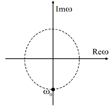
Figure 1: Analytic structure of the retarded Green’s function with a singularity in $\omega_{0}$. The dashed line illustrates the radius of convergence of the Taylor expansion around the origin.

The series of positive powers in $\omega-\omega_{0}$ can be rearranged into a series of positive powers in $\omega$. The coefficients of the latter series can be most conveniently expressed by matching the Laurent expansion to the Taylor expansion around $\omega=0$. To this end, we expand $f\left(\omega_{0}\right)\left(\omega-\omega_{0}\right)^{-1}$ around the origin. Then we match Eq. (7) with Eq. (14). In this way, we obtain e.g. for the coefficients of the constant and linear terms in $\omega$

$$\tilde{G}_{R}\left(0\right) = -\frac{f\left(\omega_{0}\right)}{\omega_{0}}+\partial_{\omega}\left.f\left(\omega\right)\right|_{\omega=\omega_{0}}-\frac{1}{2}\partial_{\omega}^{2}\left.f\left(\omega\right)\right|_{\omega=\omega_{0}}\omega_{0}+\ldots,$$

$$\partial_{\omega}\left.\tilde{G}_{R}\left(\omega\right)\right|_{\omega=0} = -\frac{f\left(\omega_{0}\right)}{\omega_{0}^{2}}+\frac{1}{2}\partial_{\omega}^{2}\left.f\left(\omega\right)\right|_{\omega=\omega_{0}}+\ldots.$$ (15)

We now observe that all constant terms in $\omega$ in Eq. (14) can be expressed as $\tilde{G}_{R}(0)+f(\omega_{0})/\omega_{0}$, while all linear terms in $\omega$ can be written as $\partial_{\omega}\tilde{G}_{R}(\omega)|_{\omega=0}+f(\omega_{0})/\omega_{0}^{2}$. Higher-order terms in $\omega$ can be expressed in a similar fashion. Thus, we can rewrite Eq. (14) in the following way

$$\tilde{G}_{R}\left(\omega\right)=\frac{f\left(\omega_{0}\right)}{\omega-\omega_{0}}+\left[\tilde{G}_{R}\left(0\right)+\frac{f\left(\omega_{0}\right)}{\omega_{0}}\right]+\left[\partial_{\omega}\left.\tilde{G}_{R}\left(\omega\right)\right|_{\omega=0}+\frac{f\left(\omega_{0}\right)}{\omega_{0}^{2}}\right]\omega+\mathcal{O}(\omega^{2}).$$ (16)

The inverse Fourier transform of $\tilde{G}_{R}\left(\omega\right)$ is straightforwardly obtained and has the form

$$G_{R}\left(t-t^{\prime}\right) = -if\left(\omega_{0}\right)\exp\left[-i\omega_{0}\left(t-t^{\prime}\right)\right]\theta\left(t-t^{\prime}\right)+\left[\tilde{G}_{R}\left(0\right)+\frac{f\left(\omega_{0}\right)}{\omega_{0}}\right]\delta\left(t-t^{\prime}\right)$$ (17)

$$+i\left[\partial_{\omega}\left.\tilde{G}_{R}\left(\omega\right)\right|_{\omega=0}+\frac{f\left(\omega_{0}\right)}{\omega_{0}^{2}}\right]\partial_{t}\delta\left(t-t^{\prime}\right)+\mathcal{O}(\partial_{t}^{2}).$$

This retarded Green’s function is the solution of the following differential equation

$$\partial_{t}G_{R}\left(t-t^{\prime}\right)+i\omega_{0}G_{R}\left(t-t^{\prime}\right) = i\omega_{0}\tilde{G}_{R}\left(0\right)\delta\left(t-t^{\prime}\right)$$ (18)

$$- \left[\omega_{0}\partial_{\omega}\left.\tilde{G}_{R}\left(\omega\right)\right|_{\omega=0}-\tilde{G}_{R}\left(0\right)\right]\partial_{t}\delta\left(t-t^{\prime}\right)+\mathcal{O}\left(\partial_{t}^{2}\right).$$

Dividing Eq. (18) by $i\omega_{0}$, multiplying by $F\left(t^{\prime}\right)$, and integrating over $t^{\prime}$, one now obtains an equation of motion for the current $J$ defined in Eq. (2), instead of a simple algebraic identity as in the gradient expansion, cf. Eq. (10). This equation of motion reads

$$\tau_{R}\partial_{t}J+J=D_{0}F+D_{1}\partial_{t}F+\mathcal{O}\left(\partial_{t}^{2}F\right),$$ (19)

where the coefficients are

$$\tau_{R} = \frac{1}{i\omega_{0}}=\frac{1}{\zeta},\text{ }$$

$$D_{0} = \tilde{G}_{R}\left(0\right),\text{ }$$

$$D_{1} = i\partial_{\omega}\left.\tilde{G}_{R}\left(\omega\right)\right|_{\omega=0}+D_{0}\tau_{R}=\tau_{R}\,\partial_{\omega}\left.f\left(\omega\right)\right|_{\omega=0}.$$ (20)

Note that, in case $\tilde{G}_{R}(\omega)$ has a single simple pole, Eq. (19) is exact.

It is clear that Eq. (19) is nothing but a relaxation equation which is similar in structure to that occurring in the transient theories for non-relativistic fluid dynamics proposed by Grad Grad and extended to relativistic fluids by Israel and Stewart in Ref. IS . The appearance of the time derivative of $J$ is due to the existence of the pole in the retarded Green’s function. Also, the transport coefficient $\tau_{R}$, usually known as the relaxation time coefficient, is directly related to the singularity, $\omega_{0}\equiv-i\zeta$, of $\tilde{G}_{R}\left(\omega\right)$. Since $\zeta>0$, $\tau_{R}$ is real and positive, as expected. It is interesting to note that $D_{0}\equiv\bar{D}_{0}$, with $\bar{D}_{0}$ from Eq. (11), while $D_{1}$ is not identical to $\bar{D}_{1}$, cf. see Eqs. (11) and (20).

It should be noted that the right-hand side of Eq. (19) can be truncated using the same procedure employed for Eq. (10). After this truncation, the dissipative current $J$ satisfies the following equation,

$$\tau_{R}\partial_{t}J+J=D_{0}F+D_{1}\partial_{t}F\;.$$ (21)

As before, it was assumed that $\mathrm{Kn}\ll 1$, with $\mathrm{Kn}$ being the appropriate Knudsen number, and terms of order $\mathcal{O}\left(\mathrm{Kn}^{3}\right)$ were dropped.

As was mentioned in the beginning of this section, the Taylor expansion around $\omega=0$ is valid in a radius $\left|\omega_{0}\right|$ around the origin, see Fig. 1. Thus, when the pole is pushed to infinity, $\left|\omega_{0}\right|\rightarrow\infty$, the radius of convergence of the Taylor series becomes infinite and we should recover the gradient expansion. In fact, taking the limit $\left|\omega_{0}\right|\rightarrow\infty$, that is, $\tau_{R}\rightarrow 0$, cf. Eqs. (20), one recovers Eq. (10), with identical coefficients. The coefficient $D_{0}$ was already seen to be identical to $\bar{D}_{0}$, while $D_{1}$ agrees with $\bar{D}_{1}$ only in the limit of vanishing relaxation time comment1 .

In the case where the thermodynamic force varies slowly on the time scale given by $\tau_{R}$, eventually, i.e., for times $t\gg\tau_{R}$, the dissipative current $J$ will follow the time dependence imposed by the right-hand side of Eq. (21). In other words, the transient term $\tau_{R}\partial_{t}J$ in Eq. (21) will become small. Then it is permissible to replace $J$ in this term by the right-hand side of Eq. (21), and we obtain up to terms of order $\mathcal{O}(\mathrm{Kn}^{3})$

$$J\simeq D_{0}F+D_{1}\partial_{t}F-\tau_{R}D_{0}\partial_{t}F\equiv\bar{D_{0}}F+\bar{D}_{1}\partial_{t}F\;,$$ (22)

i.e., we recover the result (10) given by the gradient expansion. In this sense, the gradient expansion is the asymptotic solution of Eq. (19) for time $t\gg\tau_{R}$.

For nonrelativistic systems, when the transient dynamics can be neglected at all times, it is known that the first-order truncation of the gradient expansion can actually serve not only as an asymptotic solution, but as an effective theory to describe the system, e.g., substituting the first-order result into the conservation equations one obtains the nonrelativistic diffusion equation and the nonrelativistic Navier-Stokes equation. However, for relativistic theories this is not possible because of the violation of causality. As was mentioned in the Introduction, because of Eq. (1) for any non-zero value of the transport coefficients (shear viscosity, bulk viscosity, etc.) it is not possible to take the (acausal) limit of vanishing relaxation time, if one wants to obtain causal and stable relativistic fluid-dynamical equations of motion.

IV.2 $\tilde{G}_{R}\left(\omega\right)$ with two poles

In order to better understand the consequences induced by the retarded Green’s function’s nontrivial analytic structure, it is useful to analyze in detail the case where $\tilde{G}_{R}\left(\omega\right)$ has two poles, $\omega_{1}$ and $\omega_{2}$,

$$\tilde{G}_{R}\left(\omega\right)=\frac{f_{1}\left(\omega\right)}{\omega-\omega_{1}}+\frac{f_{2}\left(\omega\right)}{\omega-\omega_{2}}.$$ (23)

We employ exactly the same steps as before and expand each term of $\tilde{G}_{R}\left(\omega\right)$ in a Laurent series around its respective pole. The result is

$$\tilde{G}_{R}\left(\omega\right) = \frac{f_{1}\left(\omega_{1}\right)}{\omega-\omega_{1}}+\frac{f_{2}\left(\omega_{2}\right)}{\omega-\omega_{2}}+\partial_{\omega}\left.f_{1}\left(\omega\right)\right|_{\omega=\omega_{1}}+\partial_{\omega}\left.f_{2}\left(\omega\right)\right|_{\omega=\omega_{2}}$$ (24)

$$+\frac{1}{2}\partial_{\omega}^{2}\left.f_{1}\left(\omega\right)\right|_{\omega=\omega_{1}}\left(\omega-\omega_{1}\right)+\frac{1}{2}\partial_{\omega}^{2}\left.f_{2}\left(\omega\right)\right|_{\omega=\omega_{2}}\left(\omega-\omega_{2}\right)+\mathcal{O}\left[(\omega-\omega_{i})^{2}\right]\,.$$

As before, we can match this expansion to the Taylor expansion near the origin. This enables us to rewrite $\tilde{G}_{R}\left(\omega\right)$ as

$$\tilde{G}_{R}\left(\omega\right)=\frac{f_{1}\left(\omega_{1}\right)}{\omega-\omega_{1}}+\frac{f_{2}\left(\omega_{2}\right)}{\omega-\omega_{2}} + \left[\tilde{G}_{R}\left(0\right)+\frac{f_{1}\left(\omega_{1}\right)}{\omega_{1}}+\frac{f_{2}\left(\omega_{2}\right)}{\omega_{2}}\right]$$ (25)

$$+ \left[\partial_{\omega}\left.\tilde{G}_{R}\left(\omega\right)\right|_{\omega=0}+\frac{f_{1}\left(\omega_{1}\right)}{\omega_{1}^{2}}+\frac{f_{2}\left(\omega_{2}\right)}{\omega_{2}^{2}}\right]\omega$$

$$+ \left[\frac{1}{2}\left.\partial_{\omega}^{2}\,\tilde{G}_{R}(\omega)\right|_{\omega=0}+\frac{f_{1}(\omega_{1})}{\omega_{1}^{3}}+\frac{f_{2}(\omega_{2})}{\omega_{2}^{3}}\right]\,\omega^{2}+\mathcal{O}(\omega^{3}).$$

With the last expression, we can determine the Green’s function $G_{R}(t-t^{\prime})$ and also its equation of motion. Similarly to the previous section, it is straightforward to show that

$$G_{R}\left(t-t^{\prime}\right) = -i\left\{\frac{{}}{{}}f_{1}\left(\omega_{1}\right)\exp\left[-i\omega_{1}\left(t-t^{\prime}\right)\right]+f_{2}\left(\omega_{2}\right)\exp\left[-i\omega_{2}\left(t-t^{\prime}\right)\right]\right\}\theta\left(t-t^{\prime}\right)$$ (26)

$$+\left[\tilde{G}_{R}\left(0\right)+\frac{f_{1}\left(\omega_{1}\right)}{\omega_{1}}+\frac{f_{2}\left(\omega_{2}\right)}{\omega_{2}}\right]\delta\left(t-t^{\prime}\right)$$

$$+i\left[\partial_{\omega}\left.\tilde{G}_{R}\left(\omega\right)\right|_{\omega=0}+\frac{f_{1}\left(\omega_{1}\right)}{\omega_{1}^{2}}+\frac{f_{2}\left(\omega_{2}\right)}{\omega_{2}^{2}}\right]\partial_{t}\delta\left(t-t^{\prime}\right)$$

$$-\left[\frac{1}{2}\,\partial_{\omega}^{2}\left.\tilde{G}_{R}(\omega)\right|_{\omega=0}+\frac{f_{1}(\omega_{1})}{\omega_{1}^{3}}+\frac{f_{2}(\omega_{2})}{\omega_{2}^{3}}\right]\,\partial_{t}^{2}\,\delta(t-t^{\prime})+\mathcal{O}(\partial_{t}^{3})\,.$$

The equation satisfied by $G_{R}$ is

$$-\partial_{t}^{2}G_{R}\left(t-t^{\prime}\right)=i\left(\omega_{1}+\omega_{2}\right)\partial_{t}G_{R}\left(t-t^{\prime}\right)-\omega_{1}\omega_{2}G_{R}\left(t-t^{\prime}\right)+\omega_{1}\omega_{2}\tilde{G}_{R}\left(0\right)\delta\left(t-t^{\prime}\right)$$ (27)

$$+ i\left[\omega_{1}\omega_{2}\partial_{\omega}\left.\tilde{G}_{R}\left(\omega\right)\right|_{\omega=0}-\left(\omega_{1}+\omega_{2}\right)\tilde{G}_{R}\left(0\right)\right]\partial_{t}\delta\left(t-t^{\prime}\right)$$

$$- \left[\frac{1}{2}\,\omega_{1}\,\omega_{2}\,\partial_{\omega}^{2}\left.\tilde{G}_{R}(\omega)\right|_{\omega=0}-\left(\omega_{1}+\omega_{2}\right)\,\partial_{\omega}\left.\tilde{G}_{R}(\omega)\right|_{\omega=0}+\tilde{G}_{R}(0)\right]\,\partial_{t}^{2}\,\delta(t-t^{\prime})+\mathcal{O}(\partial_{t}^{3})\;,\;\;\;\;$$

The main difference to the previous case is that, due to the existence of a second pole, the Green’s function now satisfies a second-order differential equation, instead of a first-order one. As will be shown later, the order of the differential equation satisfied by $\tilde{G}_{R}\left(\omega\right)$ is equal to the number of its singularities. Dividing by $-\omega_{1}\omega_{2}$, multiplying the equation by $F\left(t^{\prime}\right)$, and integrating over $t^{\prime}$ we can determine the equation of motion for $J$,

$$\chi_{2}\partial_{t}^{2}J+\chi_{1}\partial_{t}J+J=D_{0}F\left(t\right)+D_{1}\partial_{t}F\left(t\right)+D_{2}\partial_{t}^{2}F\left(t\right)+\mathcal{O}\left[\left(\lambda/\ell\right)^{4}\right].$$ (28)

We introduced the following transport coefficients,

$$\chi_{2} = -\frac{1}{\omega_{1}\omega_{2}},$$

$$\chi_{1} = \frac{1}{i\omega_{1}}+\frac{1}{i\omega_{2}},$$

$$D_{0} = \tilde{G}_{R}\left(0\right),\text{ }$$

$$D_{1} = i\partial_{\omega}\left.\tilde{G}_{R}\left(\omega\right)\right|_{\omega=0}+D_{0}\chi_{1}\,,$$

$$D_{2} = -\frac{1}{2}\partial_{\omega}^{2}\left.\tilde{G}_{R}\left(\omega\right)\right|_{\omega=0}+D_{1}\chi_{1}+D_{0}\left(\chi_{2}-\chi_{1}^{2}\right),$$ (29)

Note that $\chi_{2}$ and $\chi_{1}$ have contributions from both poles.

Next, we shall investigate under which circumstances a relaxation equation for $J$ can be obtained. Due to time reversal invariance, the two poles of $\tilde{G}_{R}\left(\omega\right)$ can appear in two ways: (i) both poles are on the imaginary axis, in which case we assume, without any loss of generality, that $\left|\omega_{2}\right|>\left|\omega_{1}\right|$; (ii) both poles have the same imaginary part, but opposite real parts, being symmetric with respect to the imaginary axis. In this case, $\left|\omega_{1}\right|=\left|\omega_{2}\right|$. See Fig. 2 for details. Both cases reflect distinct physical scenarios.

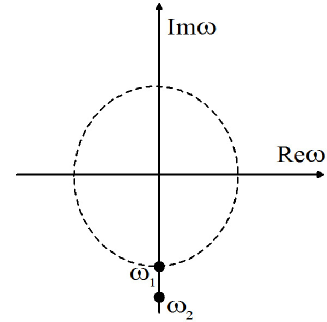
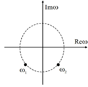
Figure 2: Analytic structure of the retarded Green’s function with two singularities, $\omega_{1}$ and $\omega_{2}$. Case (i), in which both poles are on the imaginary axis, is illustrated on the left. Case (ii), in which both poles are symmetric around the imaginary axis, is illustrated on the right. The dashed line illustrates the radius of convergence of the Taylor expansion around the origin.

Let us consider the case in which the thermodynamic force is turned off, and the current $J$ is left to relax to equilibrium. This process is governed by the equation

$$\chi_{2}\partial_{t}^{2}J+\chi_{1}\partial_{t}J+J=0.$$ (30)

This is the equation of motion of a damped harmonic oscillator,

$$\ddot{x}+2\,\gamma\,\dot{x}+\omega_{0}^{2}\,x=0\;.$$ (31)

The harmonic oscillator is overdamped, if $\gamma>\omega_{0}$, and underdamped, if $\gamma<\omega_{0}$. Identifying the coefficients, we find

$$\gamma=\frac{\chi_{1}}{2\,\chi_{2}}\;,\;\;\;\;\omega_{0}^{2}=\frac{1}{\chi_{2}}\;.$$ (32)

Therefore, if $\chi_{1}^{2}>4\,\chi_{2}$, the dissipative current $J$ relaxes to equilibrium without oscillating, while for $\chi_{1}^{2}<4\,\chi_{2}$, it relaxes in an oscillatory fashion. Using the definitions (29), we see that in the overdamped case, $4\omega_{1}\omega_{2}>(\omega_{1}+\omega_{2})^{2}$, while in the underdamped case, $4\omega_{1}\omega_{2}<(\omega_{1}+\omega_{2})^{2}$.

In case (i), both poles are purely imaginary, $\omega_{i}\equiv-i\zeta_{i}$, with $\zeta_{i}>0$, $i=1,2$. Since always $4\zeta_{1}\zeta_{2}<(\zeta_{1}+\zeta_{2})^{2}$, we are in the overdamped limit. In this case, a relaxation equation is obtained by applying the limiting procedure $\,\chi_{2}\rightarrow 0$. That is, the second pole is pushed to infinity, in which case the relaxation time is given by the inverse of the first pole,

$$\tau_{R}\equiv\chi_{1}=\frac{1}{i\omega_{1}}.$$

Naturally, this theory is only valid for frequencies that are small compared to the second pole.

In case (ii), $\left|\omega_{1}\right|=\left|\omega_{2}\right|$ and $\omega_{1}=-\omega_{2}^{\ast}$. We always have $|\omega_{1}|^{2}>(\mathrm{Im}\omega_{1})^{2}$, which can be rewritten in the form $4\omega_{1}\omega_{2}=-4|\omega_{1}|^{2}<(\omega_{1}-\omega_{1}^{\ast})^{2}=(\omega_{1}+\omega_{2})^{2}$. Thus, we are in the underdamped limit. In this case, due to the symmetries of the retarded Green’s function, one cannot disregard one of the poles while keeping the other. Thus, the term including the second time derivative of $J$ must be included (otherwise there would be no oscillation) and the full equation of motion must be solved. It is important to remark that, in this case, the coefficient $\chi_{1}$ cannot be interpreted as a relaxation time.

Note that the exponential decay of $J(t)$ in case (i) can also be seen when inserting the Green’s function $\tilde{G}_{R}(\omega)$ into Eq. (6) and performing the $\omega$ integral via contour integration, picking up the poles via the residue theorem. In case (ii), one gets an exponentially damped factor from the imaginary part of the pole, $\sim\exp(-|{\rm Im}\omega_{i}|\,t)$, and an oscillatory factor from the real part, $\sim\exp(i\,{\rm Re}\omega_{i}\,t)$. If $|{\rm Im}\omega_{i}|\gg|{\rm Re}\omega_{i}|$, the damping is much stronger than the oscillation, already within a single oscillation, the dissipative current has decayed a couple of $e-$folds towards its stationary solution. On the other hand, if $|{\rm Im}\omega_{i}|\ll|{\rm Re}\omega_{i}|$, the current will oscillate many times before a substantial decay occurs. The oscillatory behavior of the dissipative current in case (ii) was already noticed in Ref. Kovtun:2005ev .

It is clear from this analysis that the derivation of relaxation equations for systems with more than one pole is not possible if the first pole does not lie on the imaginary axis. With this in mind, we can finally consider the general case of an arbitrary number of poles. The result will be qualitatively similar to what was found above.

IV.3 $\tilde{G}_{R}\left(Q\right)$ with $N$ poles

Now we assume that $\tilde{G}_{R}\left(Q\right)$ has $N$ poles in the complex $\omega$-plane, $\omega_{1}\left(\mathbf{q}\right)$, … , $\omega_{N}\left(\mathbf{q}\right)$. We furthermore restore the $\mathbf{q}$ dependence which was neglected in the previous sections, and assume that the Green’s function is analytic in $\mathbf{q}$. Since $J$ is not a conserved quantity, we can safely assume that all poles remain within a finite distance from the origin even when $\mathbf{q}\rightarrow 0$. Here we consider the case of a finite (but arbitrarily large) number of poles. Also, in many cases $\tilde{G}_{R}\left(Q\right)$ contains branch cuts. We assume that these branch cuts are located further from the origin of the complex frequency plane than these $N$ poles and thus will not be considered any further in this work. The retarded Green’s function can be written in the general form

$$\tilde{G}_{R}\left(Q\right)=\sum_{i=1}^{N}\frac{f_{i}\left(Q\right)}{\omega-\omega_{i}\left(\mathbf{q}\right)}=\frac{\Xi\left(Q\right)}{\left[\omega-\omega_{1}\left(\mathbf{q}\right)\right]\cdots\left[\omega-\omega_{N}\left(\mathbf{q}\right)\right]},$$ (33)

where the $f_{i}\left(Q\right)$ and $\Xi\left(Q\right)$ are analytic functions in the complex $\omega$ plane. We now use the identity

$$1+\Phi_{1}\left(\mathbf{q}\right)\left(-i\omega\right)+\ldots+\Phi_{N}\left(\mathbf{q}\right)\left(-i\omega\right)^{N}=\left(-1\right)^{N}\frac{\left[\omega-\omega_{1}\left(\mathbf{q}\right)\right]\cdots\left[\omega-\omega_{N}\left(\mathbf{q}\right)\right]}{\omega_{1}\left(\mathbf{q}\right)\cdots\omega_{N}\left(\mathbf{q}\right)}\;,$$ (34)

where

$$\Phi_{m}\left(\mathbf{q}\right)=\left(-i\right)^{m}\sum_{1\leq i_{1}...<i_{m}\leq N}\frac{1}{\omega_{i_{1}}\left(\mathbf{q}\right)\cdots\omega_{i_{m}}\left(\mathbf{q}\right)}\;.$$ (35)

From this expression, we can find the following equation for $\tilde{G}_{R}\left(Q\right)$,

$$\left[1+\Phi_{1}\left(\mathbf{q}\right)\left(-i\omega\right)+\ldots+\Phi_{N}\left(\mathbf{q}\right)\left(-i\omega\right)^{N}\right]\tilde{G}_{R}\left(Q\right)=\frac{\left(-1\right)^{N}\Xi\left(Q\right)}{\omega_{1}\left(\mathbf{q}\right)\cdots\omega_{N}\left(\mathbf{q}\right)}\;.$$ (36)

After taking the Fourier transform and expanding the functions $\Phi_{m}\left(\mathbf{q}\right)$ in a Taylor series around $\mathbf{q}=0$, we obtain a differential equation satisfied by $G_{R}$. It is clear that this will be a linear differential equation of order $N$ in time. The equation of motion for $J$ can be obtained in the same way as before. The result is

$$\chi_{N}\partial_{t}^{N}J+\ldots+\chi_{1}\partial_{t}J+J=D_{0}F+\ldots+D_{N}\partial_{t}^{N}F+\mathcal{O}\left(\partial_{t}^{N+1}F,\partial_{\mathbf{x}}\right).$$ (37)

Here, we omitted all the terms involving spatial derivatives. The coefficients $\chi_{m}$ are

$$\chi_{m}=\Phi_{m}\left(\mathbf{0}\right)=\left(-i\right)^{m}\sum_{1\leq i_{1}...<i_{m}\leq N}\frac{1}{\omega_{i_{1}}\left(\mathbf{0}\right)\cdots\omega_{i_{m}}\left(\mathbf{0}\right)}\;.$$ (38)

As before, the coefficients $D_{0}$, $D_{1}$ and $D_{2}$ can be expressed as

$$D_{0} = \left.\tilde{G}_{R}\left(\omega,\mathbf{0}\right)\right|_{\omega=0}\;,$$

$$D_{1} = i\partial_{\omega}\left.\tilde{G}_{R}\left(\omega,\mathbf{0}\right)\right|_{\omega=0}+D_{0}\chi_{1}\;,$$

$$D_{2} = -\frac{1}{2}\partial_{\omega}^{2}\left.\tilde{G}_{R}\left(\omega,\mathbf{0}\right)\right|_{\omega=0}+D_{1}\chi_{1}+D_{0}\left(\chi_{2}-\chi_{1}^{2}\right)\;,$$ (39)

cf. Eq. (29). In general, the coefficients $D_{k}$ have the following form

$$D_{k}=i^{k}\frac{\left(-1\right)^{N}}{k!}\frac{\partial_{\omega}^{k}\left.\Xi\left(\omega,\mathbf{0}\right)\right|_{\omega=0}}{\omega_{1}\left(\mathbf{0}\right)\cdots\omega_{N}\left(\mathbf{0}\right)}.$$ (40)

We remark that up to now we have not employed any approximation besides the initial assumptions regarding the singularities of $\tilde{G}_{R}$. As mentioned before, if there is a clear separation of scales, it is possible to simplify the equation of motion. Since $D_{n}\sim\lambda^{n+1}$, assuming that $\lambda/\ell\ll 1$, we can safely assume $D_{0}F\gg D_{1}\partial_{t}F\gg D_{2}\partial_{t}^{2}F$ and truncate the right-hand side of Eq. (37).

As discussed in the previous section, a relaxation equation can be obtained only for the cases in which the pole nearest to the origin (in the following referred to as the “first pole”) lies on the imaginary axis. In this case, the limiting procedure which pushes all the other poles to infinity, $\chi_{i}\rightarrow 0$, $i\geq 2$, can be applied without breaking any symmetries of the retarded Green’s function. Assuming that this can be done, we obtain the following equation of motion for $J$

$$\tau_{R}\partial_{t}J+J=D_{0}F+D_{1}\partial_{t}F+D_{2}\partial_{t}^{2}F+\mathcal{O}\left(D_{3}\partial_{t}^{3}F,\partial_{\mathbf{x}}\right)\;.$$ (41)

where

$$\tau_{R} = \frac{1}{i\omega_{1}\left(\mathbf{0}\right)},$$

$$D_{0} = \left.\tilde{G}_{R}\left(\omega,\mathbf{0}\right)\right|_{\omega=0}\;,$$

$$D_{1} = i\partial_{\omega}\left.\tilde{G}_{R}\left(\omega,\mathbf{0}\right)\right|_{\omega=0}+D_{0}\,\tau_{R}\;,$$

$$D_{2} = -\frac{1}{2}\partial_{\omega}^{2}\left.\tilde{G}_{R}\left(\omega,\mathbf{0}\right)\right|_{\omega=0}+D_{1}\,\tau_{R}-D_{0}\,\tau_{R}^{2}\;,$$ (42)

On the other hand, if the first pole and, for reasons of symmetry, its counterpart on the other side of the imaginary axis, have nonzero real parts, the dissipative current will oscillate and the equation of motion cannot be reduced to a simple relaxation equation, even in the small-frequency domain.

V Applications

V.1 The Linearized Boltzmann Equation

The discussion presented above is valid for both weakly and strongly coupled theories. The prime example of a weakly coupled theory is given by the Boltzmann equation. In this section we calculate the shear viscosity and relaxation time coefficients for a weakly coupled gas via the Boltzmann equation following the general method presented above.

We start from the relativistic Boltzmann equation

$$K\cdot\partial f_{\mathbf{k}}=C\left[f\right],$$ (43)

where $K=(k_{0},\mathbf{k})$, $k_{0}=\sqrt{\mathbf{k}^{2}+m^{2}}$, and $m$ is the particle mass. We use the notation $f_{\mathbf{k}}\left(X\right)=f\left(X,K\right)$. We consider the linearized Boltzmann equation around the classical equilibrium state, $f_{0\mathbf{k}}\equiv$ $\exp\left(y_{0\mathbf{k}}\right)$, where $y_{0\mathbf{k}}=\alpha_{0}-\beta_{0}E_{\mathbf{k}}$, with the inverse temperature $\beta_{0}$, the ratio of the chemical potential to temperature $\alpha_{0}$, and the energy in the local rest frame $E_{\mathbf{k}}\equiv U\cdot K$, respectively. Here, $u^{\mu}$ is the fluid four-velocity.

The Boltzmann equation can be written as

$$\delta\dot{f}_{\mathbf{k}}+E_{\mathbf{k}}^{-1}K\cdot\nabla\delta f_{\mathbf{k}}-\hat{C}\left(X,K\right)\delta f_{\mathbf{k}}=\mathcal{S}\left(X,K\right),$$ (44)

where we defined $\delta f_{\mathbf{k}}\equiv f_{\mathbf{k}}-f_{0\mathbf{k}}$, $\dot{A}\equiv U\cdot\partial A$, $\nabla_{\mu}\equiv\Delta_{\mu\nu}\partial^{\nu}$, with $\Delta^{\mu\nu}=\eta^{\mu\nu}-u^{\mu}u^{\nu}$ being the 3-space projector orthogonal to $u^{\mu}$, and

$$\mathcal{S}\left(X,K\right) \equiv f_{0\mathbf{k}}\left[-\dot{\alpha}_{0}+E_{\mathbf{k}}\dot{\beta}_{0}+K\cdot\left(\beta_{0}\dot{U}+\nabla\beta_{0}-E_{\mathbf{k}}^{-1}\nabla\alpha_{0}\right)\right.$$ (45)

$$\left.+\frac{\beta_{0}}{3}E_{\mathbf{k}}^{-1}\left(m^{2}-E_{\mathbf{k}}^{2}\right)\theta+\beta_{0}E_{\mathbf{k}}^{-1}k^{\left\langle\mu\right.}k^{\left.\nu\right\rangle}\sigma_{\mu\nu}\right].$$

Here, we introduced the expansion scalar $\theta\equiv\partial\cdot U$ and the shear tensor $\sigma^{\mu\nu}\equiv\nabla^{\left\langle\mu\right.}u^{\left.\nu\right\rangle}$, where $A^{\left\langle\mu\nu\right\rangle}=\Delta^{\mu\nu\alpha\beta}A_{\alpha\beta}$ with $\Delta^{\mu\nu\alpha\beta}=\left(\Delta^{\mu\alpha}\Delta^{\nu\beta}+\Delta^{\mu\beta}\Delta^{\nu\alpha}\right)/2-\Delta^{\mu\nu}\Delta^{\alpha\beta}/3$ being the double symmetric traceless projection operator. In Eq. (44), we also introduced the collision operator

$$\hat{C}\left(X,K\right)\delta f_{\mathbf{k}}=\frac{1}{\nu E_{\mathbf{k}}}\int dK^{\prime}dPdP^{\prime}W_{\mathbf{kk}\prime\rightarrow\mathbf{pp}\prime}f_{0\mathbf{k}}f_{0\mathbf{k}^{\prime}}\left(\frac{\delta f_{\mathbf{p}^{\prime}}}{f_{0\mathbf{p}^{\prime}}}+\frac{\delta f_{\mathbf{p}}}{f_{0\mathbf{p}}}-\frac{\delta f_{\mathbf{k}^{\prime}}}{f_{0\mathbf{k}^{\prime}}}-\frac{\delta f_{\mathbf{k}}}{f_{0\mathbf{k}}}\right),$$ (46)

where $W_{\mathbf{kk}\prime\rightarrow\mathbf{pp}\prime}$ is the transition rate, $\nu$ is the symmetry factor ($\nu=2$ for identical particles) and

$$dK=\frac{d^{3}\mathbf{k}}{\left(2\pi\right)^{3}E_{\mathbf{k}}}.$$ (47)

We now consider Eq. (44) in the local rest frame, where $U=(1,0,0,0)$. We assume a situation where the fluid does not accelerate, $\dot{U}\equiv 0$, and does not expand, $\theta\equiv 0$, and where temperature and chemical potential are constant. With these assumptions the source term reduces to

$$\mathcal{S}\left(X,K\right)=\beta_{0}f_{0\mathbf{k}}E_{\mathbf{k}}^{-1}k^{\left\langle\mu\right.}k^{\left.\nu\right\rangle}\sigma_{\mu\nu}\left(X\right)\;,$$ (48)

and the collision operator no longer depends on $X$, $\hat{C}(X,K)\equiv\hat{C}(K)$. The Boltzmann equation (44) takes the form

$$\partial_{t}\delta f_{\mathbf{k}}+\mathbf{v}\cdot\nabla\delta f_{\mathbf{k}}-\hat{C}\left(K\right)\delta f_{\mathbf{k}}=\mathcal{S}\left(X,K\right)\;,$$ (49)

where $\mathbf{v}\equiv\mathbf{k}/E_{\mathbf{k}}$.

We solve the inhomogeneous, linear, partial integro-differential equation (49) for $\delta f_{\mathbf{k}}$ in four-momentum space. Taking the Fourier transform we obtain

$$-i\omega\delta\tilde{f}_{\mathbf{k}}\left(Q\right)+i\mathbf{v}\cdot\mathbf{q}\,\delta\tilde{f}_{\mathbf{k}}\left(Q\right)-\hat{C}\left(K\right)\delta\tilde{f}_{\mathbf{k}}\left(Q\right)=\mathcal{\tilde{S}}\left(Q,K\right)\,.$$ (50)

From now on, it is important not to confuse the momenta of the particles, $K$, $K^{\prime}$, $P$, and $P^{\prime}$, with the variable $Q$ from the Fourier transformation.

The formal solution of Eq. (50) can be expressed in the following form

$$\delta\tilde{f}_{\mathbf{k}}\left(Q\right)=\frac{1}{-i\omega+i\mathbf{v}\cdot\mathbf{q}-\hat{C}\left(K\right)}\mathcal{\tilde{S}}\left(Q,K\right).$$ (51)

Note that the shear stress tensor, $\pi^{\mu\nu}$, can be expressed in terms of $\delta f_{\mathbf{k}}$ as dkr

$$\pi^{\mu\nu}=\int dK\,k^{\left\langle\mu\right.}k^{\left.\nu\right\rangle}\delta f_{\mathbf{k}}.$$ (52)

Taking the Fourier transform of Eq. (52) and using Eqs. (48) and (51), we obtain

$$\tilde{\pi}^{\mu\nu}\left(Q\right)=\int dK\,k^{\left\langle\mu\right.}k^{\left.\nu\right\rangle}\frac{1}{-i\omega+i\mathbf{v}\cdot\mathbf{q}-\hat{C}\left(K\right)}\beta_{0}f_{0\mathbf{k}}E_{\mathbf{k}}^{-1}k^{\left\langle\alpha\right.}k^{\left.\beta\right\rangle}\tilde{\sigma}_{\alpha\beta}\left(Q\right).$$ (53)

Note that Eq. (53) has the following form,

$$\tilde{\pi}^{\mu\nu}\left(Q\right)=\tilde{G}_{R}^{\mu\nu\alpha\beta}\left(Q\right)\tilde{\sigma}_{\alpha\beta}\left(Q\right),$$ (54)

where we introduced

$$\tilde{G}_{R}^{\mu\nu\alpha\beta}\left(Q\right)=\int dK\,k^{\left\langle\mu\right.}k^{\left.\nu\right\rangle}\frac{1}{-i\omega+i\mathbf{v}\cdot\mathbf{q}-\hat{C}\left(K\right)}\beta_{0}f_{0\mathbf{k}}E_{\mathbf{k}}^{-1}k^{\left\langle\alpha\right.}k^{\left.\beta\right\rangle}.$$ (55)

As already mentioned, we want to calculate the two main transport coefficients that describe the linearized dynamics of the shear stress tensor: the shear relaxation time, $\tau_{\pi}$, and the shear viscosity coefficient, $\eta$. Let us start by defining the function

$$B^{\alpha\beta}=\frac{1}{-i\omega+i\mathbf{v}\cdot\mathbf{q}-\hat{C}\left(K\right)}\beta_{0}f_{0\mathbf{k}}E_{\mathbf{k}}^{-1}k^{\left\langle\alpha\right.}k^{\left.\beta\right\rangle},$$ (56)

where, by definition, $B^{\alpha\beta}$ satisfies

$$\left[-i\omega+i\mathbf{v}\cdot\mathbf{q}-\hat{C}\left(K\right)\right]B^{\alpha\beta}\left(Q,K\right)=\beta_{0}E_{\mathbf{k}}^{-1}k^{\left\langle\alpha\right.}k^{\left.\beta\right\rangle}f_{0\mathbf{k}}.$$ (57)

In general, $B^{\alpha\beta}$ is a function of $Q$ and $K$. However, from Eqs. (38) and (39) we already know that, in order to calculate the relaxation time and the viscosity coefficient, it is sufficient to consider the case $\mathbf{q}=0$. Then $B^{\alpha\beta}=B^{\alpha\beta}\left(\omega,K\right)$. The dependence of $B^{\alpha\beta}$ on $K$ can be expressed via the following expansion,

$$B^{\alpha\beta}\left(\omega,K\right)=f_{0\mathbf{k}}k^{\left\langle\alpha\right.}k^{\left.\beta\right\rangle}\sum_{n=0}^{\infty}a_{n}\left(\omega\right)E_{\mathbf{k}}^{n}.$$ (58)

Substituting Eq. (58) into Eq. (55), it follows that

$$\tilde{G}_{R}^{\mu\nu\alpha\beta}\left(\omega,\mathbf{0}\right) = \sum_{n=0}^{\infty}a_{n}\left(\omega\right)\int dK\,k^{\left\langle\mu\right.}k^{\left.\nu\right\rangle}k^{\left\langle\alpha\right.}k^{\left.\beta\right\rangle}E_{\mathbf{k}}^{n}f_{0\mathbf{k}}$$ (59)

$$= 2\Delta^{\mu\nu\alpha\beta}\sum_{n=0}^{\infty}I_{n+4,2}\;a_{n}\left(\omega\right)\,,$$

where we used DeGroot

$$\int dK\,k^{\left\langle\mu\right.}k^{\left.\nu\right\rangle}k^{\left\langle\alpha\right.}k^{\left.\beta\right\rangle}E_{\mathbf{k}}^{n}f_{0\mathbf{k}}=\frac{2}{5!!}\,\Delta^{\mu\nu\alpha\beta}\int dK\,E_{\mathbf{k}}^{n}f_{0\mathbf{k}}\left(m^{2}-E_{\mathbf{k}}^{2}\right)^{2}\;,$$ (60)

and introduced the thermodynamic function

$$I_{nq}=\frac{1}{\left(2q+1\right)!!}\int dKf_{0\mathbf{k}}E_{\mathbf{k}}^{n-2q}\left(m^{2}-E_{\mathbf{k}}^{2}\right)^{q}.$$ (61)

Thus, Eq. (54) can be cast into a more convenient form

$$\tilde{\pi}^{\mu\nu}\left(\omega,\mathbf{0}\right)=2\tilde{G}_{R}\left(\omega,\mathbf{0}\right)\tilde{\sigma}^{\mu\nu}\left(\omega,\mathbf{0}\right),$$ (62)

where we introduced the retarded Green’s function

$$\tilde{G}_{R}\left(\omega,\mathbf{0}\right)=\sum_{n=0}^{\infty}\,I_{n+4,2}\,a_{n}\left(\omega\right)\text{.}$$ (63)

Since in fluid dynamics the thermodynamic force related to the shear stress tensor is defined as $2\tilde{\sigma}^{\mu\nu}$, we kept the factor $2$ in Eq. (62). As shown in the previous section, Eqs. (38) and (39), the shear relaxation time is determined by the first pole, $\omega_{1}$, of $\tilde{G}_{R}\left(\omega,\mathbf{0}\right)$, as

$$\tau_{\pi}=\frac{1}{i\omega_{1}\left(\mathbf{0}\right)},$$ (64)

while the shear viscosity coefficient is determined by the retarded Green’s function $\tilde{G}_{R}\left(\omega,\mathbf{0}\right)$ at the origin,

$$\eta=\left.\tilde{G}_{R}\left(\omega,\mathbf{0}\right)\right|_{\omega=0}\;.$$ (65)

Thus, the problem of finding the linear transport coefficients has been reduced to determining the analytic properties of $a_{n}\left(\omega\right)$.

Equations such as Eq. (57) appear quite often in problems involving the extraction of transport coefficients from the Boltzmann equation. The way to solve this problem is to substitute the expansion (58) into Eq. (57), multiply by $E_{\mathbf{k}}^{m}k^{\left\langle\mu\right.}k^{\left.\nu\right\rangle}$, and integrate over $dK$. Then one obtains

$$\sum_{n=0}^{\infty}a_{n}\left(\omega\right)\int dKE_{\mathbf{k}}^{m}k^{\left\langle\mu\right.}k^{\left.\nu\right\rangle}\left[-i\omega-\hat{C}\left(K\right)\right]f_{0\mathbf{k}}E_{\mathbf{k}}^{n}k^{\left\langle\alpha\right.}k^{\left.\beta\right\rangle}$$ (66)

$$= \beta_{0}\int dKE_{\mathbf{k}}^{m-1}k^{\left\langle\mu\right.}k^{\left.\nu\right\rangle}k^{\left\langle\alpha\right.}k^{\left.\beta\right\rangle}f_{0\mathbf{k}}\;,$$

Using Eqs. (60) and (61), we can rewrite this in the form

$$\sum_{n=0}^{\infty}\left(-i\omega\mathcal{D}^{mn}+\mathcal{A}^{mn}\right)a_{n}\left(\omega\right)=\beta_{0}I_{m+3,2}\;,$$ (67)

where we defined the matrices

$$\mathcal{A}^{mn}\Delta^{\mu\nu\alpha\beta} = -\frac{1}{2}\int dKE_{\mathbf{k}}^{m}k^{\left\langle\mu\right.}k^{\left.\nu\right\rangle}\hat{C}\left(K\right)f_{0\mathbf{k}}E_{\mathbf{k}}^{n}k^{\left\langle\alpha\right.}k^{\left.\beta\right\rangle},$$ (68)

$$\mathcal{D}^{mn} = \frac{1}{5!!}\int dKf_{0\mathbf{k}}E_{\mathbf{k}}^{m+n}\left(m^{2}-E_{\mathbf{k}}^{2}\right)^{2}\,.$$ (69)

Thus, the formal solution for $a_{n}(\omega)$ is

$$a_{m}\left(\omega\right)=\beta_{0}\sum_{n=0}^{\infty}\left[\left(-i\omega\mathcal{D}+\mathcal{A}\right)^{-1}\right]^{mn}I_{n+3,2}$$ (70)

and the expression for $\tilde{G}_{R}\left(\omega,\mathbf{0}\right)$ becomes

$$\tilde{G}_{R}\left(\omega,\mathbf{0}\right)=\beta_{0}\sum_{m=0}^{\infty}\sum_{n=0}^{\infty}I_{m+4,2}\left[\left(-i\omega\mathcal{D}+\mathcal{A}\right)^{-1}\right]^{mn}I_{n+3,2}.$$ (71)

The poles of the function above can be obtained from the roots of the determinant

$$\det\left(-i\omega\mathcal{D}+\mathcal{A}\right)=0\,,$$ (72)

which is given by the product of the eigenvalues $\lambda_{n}$ of the operator $\left(-i\omega\mathcal{D}+\mathcal{A}\right)$. Note that, because $\mathcal{D}$ and $\mathcal{A}$ are real matrices, all the poles are on the imaginary axis. Thus, the truncation of the equation of motion to a relaxation-type form is possible, if the separation between the poles is large enough. The shear viscosity coefficient is given by

$$\eta\equiv\left.\tilde{G}_{R}\left(\omega,\mathbf{0}\right)\right|_{\omega=0}=\beta_{0}\sum_{m=0}^{\infty}\sum_{n=0}^{\infty}I_{m+4,2}(\mathcal{A}^{-1})^{mn}I_{n+3,2}\,.$$ (73)

Thus, in order to find the relaxation times and viscosity coefficients from the linearized Boltzmann equation one has to invert and compute eigenvalues of infinite matrices. In practice, however, one never deals with infinite matrices because the expansion (58) is always truncated, see, e.g., Chapman-Enskog theory DeGroot .

Let us consider the simplest possible case and take only one term in the expansion (58). We remark that this corresponds to using the Israel-Stewart 14-moment approximation in the moments method. Then, $\tilde{G}_{R}\left(\omega,\mathbf{0}\right)$ has the following simple form

$$\tilde{G}_{R}\left(\omega,\mathbf{0}\right)=\frac{i\beta_{0}I_{32}}{\omega+i\mathcal{A}^{00}/I_{42}}\;.$$ (74)

where we used that $\mathcal{D}^{00}=I_{42}$. In this case, the retarded Green’s function has only one pole, $\omega_{0}=-i\mathcal{A}^{00}/I_{42}$. The relaxation time is obtained as

$$\tau_{\pi}=\frac{1}{i\omega_{0}}=\frac{I_{42}}{\mathcal{A}^{00}}\;.$$ (75)

On the other hand, the shear viscosity is given by $\eta=\left.\tilde{G}_{R}\left(\omega,\mathbf{0}\right)\right|_{\omega=0}$ and becomes

$$\eta=\beta_{0}\frac{I_{42}I_{32}}{\mathcal{A}^{00}}\;.$$ (76)

In the massless limit, for a gas of hard spheres, one determines $\mathcal{A}^{00}$ to be

$$\mathcal{A}^{00}=\frac{3}{5}\,I_{42}\,n_{0}\,\sigma\,,$$ (77)

where $\sigma$ is the total cross section and $n_{0}$ is the particle number density. Then,

$$\eta = \frac{4}{3\sigma\beta_{0}}\;,$$ (78)

$$\tau_{\pi} = \frac{5}{3n_{0}\sigma}\;,$$ (79)

where we used that, in the massless limit,

$$I_{42} = 4\frac{P_{0}}{\beta_{0}^{2}}\;,$$ (80)

$$I_{32} = \frac{4}{5}\frac{P_{0}}{\beta_{0}}\;,$$ (81)

where $P_{0}$ is the thermodynamic pressure. Also, in this particular example, one can show that the ratio $\eta/\tau_{\pi}$ is independent of the cross section,

$$\frac{\eta}{\tau_{\pi}}=\beta_{0}I_{32}\;.$$ (82)

These are exactly the results obtained in Ref. dkr . This demonstrates that the relaxation time in IS theories, which determines the time scale of the transient dynamics of the dissipative currents, is indeed a microscopic and not a fluid-dynamical time scale. It is determined by the interparticle scattering rate, and not by the time scales of fluid dynamics located near the origin of the complex $\omega-$plane. We shall demonstrate in Sec. VI that attempts to extract the value of the relaxation time from the dynamics on fluid-dynamical time scales in general fail to give the correct expression.

It is important to remark that by including more terms in the expansion (58) we obtain a retarded Green’s function with more poles. Furthermore, the expression for the first pole and, consequently, the relaxation time, will also be modified. All the other transport coefficients will also receive corrections.

V.2 Linear Response Theory and Metric Perturbations

We now apply our formalism to the case studied in Ref. BRSSS , where the transport coefficients are determined from perturbations $h^{\mu\nu}$ of the metric tensor

$$g^{\mu\nu}=\eta^{\mu\nu}+h^{\mu\nu}\text{.}$$ (83)

This method can be equally applied at strong and weak coupling. The variation of the energy-momentum tensor $T^{\mu\nu}$ due to the metric perturbations is starinets

$$\delta T^{\mu\nu}\left(X\right)=\frac{1}{2}\int_{-\infty}^{\infty}d^{4}X^{\prime}\,G_{R}^{\mu\nu\alpha\beta}\left(X-X^{\prime}\right)\,h_{\alpha\beta}\left(X^{\prime}\right),$$ (84)

where $G_{R}^{\mu\nu\alpha\beta}\left(X-X^{\prime}\right)$ is the retarded Green’s function.

For the sake of simplicity, a very peculiar type of metric perturbation is considered, $h_{xy}=h_{xy}\left(t,z\right)$, with all other components of the metric tensor left unperturbed BRSSS ; guymoore . For this specific type of metric perturbation, all the other components of $\delta T^{\mu\nu}$ decouple from the $xy$ component and one arrives at a very simple expression for $\delta T^{xy}$ starinets

$$\delta T^{xy}(t,z)=\int_{-\infty}^{\infty}dt^{\prime}\,dz^{\prime}\,G_{R}^{xyxy}\left(t-t^{\prime};\,z-z^{\prime}\right)h_{xy}\left(t^{\prime},z^{\prime}\right).$$ (85)

The energy-momentum tensor $T^{\mu\nu}$ is then assumed to have the traditional fluid-dynamical structure

$$T^{\mu\nu}=\varepsilon\,u^{\mu}u^{\nu}-\Delta^{\mu\nu}P+\pi^{\mu\nu}\;.$$ (86)

For the particular metric perturbation considered here, the effects of bulk viscosity can be neglected without loss of generality. It is possible to show that

$$\delta T^{xy}\equiv T^{xy}(\eta^{\mu\nu}+h^{\mu\nu})-T^{xy}(\eta^{\mu\nu})=-P_{0}\,h^{xy}+\delta\pi^{xy}\;.$$ (87)

where $\delta\pi^{xy}$ is the $xy$ component of the shear stress tensor generated by the metric perturbations and $P_{0}$ is the pressure of the unperturbed state. For the sake of simplicity, the shear stress tensor of the unperturbed state is set to zero. Also, it is easy to see, using the equations of motion, that the velocity terms in the energy-momentum tensor do not contribute to $\delta T^{xy}$. Thus, we arrive at the following equation

$$\delta\pi^{xy}=P_{0}\,h^{xy}+\int_{-\infty}^{\infty}dt^{\prime}\,dz^{\prime}\,G_{R}^{xyxy}\left(t-t^{\prime};\,z-z^{\prime}\right)h_{xy}\left(t^{\prime},z^{\prime}\right).$$ (88)

After taking the Fourier transform we can show that

$$\delta\tilde{\pi}^{xy}(Q)=\tilde{G}_{R}(Q)\,\tilde{h}_{xy}(Q)\;,$$ (89)

where $\tilde{G}_{R}(Q)=-P_{0}+\tilde{G}_{R}^{xyxy}(Q)$. Note that $h^{xy}=-h_{xy}$. Since the pressure has no dependence on $Q$, it is clear that $\tilde{G}_{R}(Q)$ has the same analytic structure as $\tilde{G}_{R}^{xyxy}(Q)$.

Assuming that $\tilde{G}_{R}^{xyxy}$ has $N$ poles, $\omega_{i}(\mathbf{q})$, and that the first pole is purely imaginary, we can apply Eq. (41) and obtain the equation of motion for $\delta\pi^{xy}$,

$$\tau_{\pi}\partial_{t}\delta\pi^{xy}+\delta\pi^{xy}=D_{0}h_{xy}+D_{1}\partial_{t}h_{xy}+D_{2}\partial_{t}^{2}h_{xy}+\mathcal{O}\left(\partial_{t}^{3}h_{xy},\partial_{z}^{2}h_{xy}\right)\;.$$ (90)

Note that if the first pole is not purely imaginary, a simple relaxation equation would not be able to describe the transient dynamics, even for long times. In Eq. (90), we introduced the following transport coefficients,

$$\tau_{\pi} = \frac{1}{i\omega_{1}\left(\textbf{0}\right)}\;,$$

$$D_{0} = \left.\tilde{G}_{R}\left(\omega,\textbf{0}\right)\right|_{\omega=0}=-P_{0}+\left.\tilde{G}_{R}^{xyxy}(\omega,\textbf{0})\right|_{\omega=0}\equiv-P_{0}+P_{0}=0\;,$$

$$D_{1} = i\partial_{\omega}\left.\tilde{G}_{R}\left(\omega,\textbf{0}\right)\right|_{\omega=0}+\tau_{\pi}\,D_{0}=i\partial_{\omega}\left.\tilde{G}_{R}\left(\omega,\textbf{0}\right)\right|_{\omega=0}\equiv\eta\text{ },$$

$$D_{2} = -\frac{1}{2}\partial_{\omega}^{2}\left.\tilde{G}_{R}\left(\omega,\textbf{0}\right)\right|_{\omega=0}+D_{1}\tau_{\pi}-D_{0}\tau_{\pi}^{2}\equiv-\frac{1}{2}\partial_{\omega}^{2}\left.\tilde{G}_{R}\left(\omega,\mathbf{0}\right)\right|_{\omega=0}+\eta\tau_{\pi}\;,$$ (91)

The expression for the shear viscosity $\eta$ is now different from the one in the Boltzmann case, because $2\sigma^{xy}\equiv\partial_{t}h_{xy}$, so that the coefficient of the shear tensor is actually $D_{1}$ (and not $D_{0}$, as before). On the other hand, the relaxation time is still given by the inverse of the first pole.

VI Discussion

Relaxation-type equations for the dissipative currents have been recently derived in Ref. BRSSS . We give a brief account of the strategy employed in that work in terms of our notation. The starting point is the gradient expansion (10), assuming that a Knudsen number counting as explained at the end of Sec. III is applicable. The gradient expansion (10) is not an equation of motion for the dissipative current, but one can construct one by taking the first-order solution, $J=\bar{D}_{0}\,F+\mathcal{O}(\mathrm{Kn}^{2})$, and then replacing the first time derivative of $F$ on the right-hand side by a time derivative of $J$,

$$J=\bar{D}_{0}\,F+\bar{D}_{1}\,\partial_{t}\left(\frac{J}{\bar{D}_{0}}\right)+\mathcal{O}(\mathrm{Kn}^{3})\;\;\;\;\Longleftrightarrow\;\;\;\;\bar{\tau}_{R}\,\partial_{t}J+J\simeq\bar{D}_{0}\,F\;,$$ (92)

where $\bar{\tau}_{R}\equiv-\bar{D}_{1}/\bar{D}_{0}$ has the dimension of time. By construction, this is a relaxation-type equation of motion for the dissipative current $J$, with a relaxation time $\bar{\tau}_{R}$.

From our previous discussion, however, it is clear that this need not be the correct equation of motion for the dissipative current. If the poles of the retarded Green’s function $\tilde{G}_{R}(\omega)$ associated with the dissipative current $J$ are off the imaginary axis, the equation of motion for $J$ is never of relaxation type, and the above way to construct one is misleading, since it fails to capture the correct physics. Only if the first pole of $\tilde{G}_{R}(\omega)$ lies on the imaginary axis and is sufficiently separated from the other singularities, one can obtain a relaxation-type equation for $J$. In this case, however, the true relaxation time is $\tau_{R}=1/[i\omega_{1}(\mathbf{0})]$, and not $\bar{\tau}_{R}=-\bar{D}_{1}/\bar{D}_{0}$.

There is, however, a particular case, where $\tau_{R}=\bar{\tau}_{R}$, namely when $D_{1}=0$, i.e., when $\Xi(\omega,\mathbf{0})=const.$. This is most easily seen in the one-pole case, where, cf. Eq. (20),

$$0=i\left.\partial_{\omega}\tilde{G}_{R}(\omega,\mathbf{0})\right|_{\omega=0}+D_{0}\,\tau_{R}\equiv\bar{D}_{1}+\bar{D}_{0}\,\tau_{R}\;,$$ (93)

i.e., $\tau_{R}=-\bar{D}_{1}/\bar{D}_{0}\equiv\bar{\tau}_{R}$.

This argument can also be applied to the case discussed in Sec. V.2, where the thermodynamic force is not given by $F$ but by $\partial_{t}F$. Then, $D_{0}=0$, and $D_{1}=\bar{D}_{1}=\eta$ is the transport coefficient. In this case, $\bar{\tau}_{\pi}=-\bar{D}_{2}/\bar{D}_{1}$, and equivalency to the true relaxation time requires that $D_{2}=0$, i.e.,

$$0=-\frac{1}{2}\partial_{\omega}^{2}\left.\tilde{G}_{R}\left(\omega,\mathbf{0}\right)\right|_{\omega=0}+D_{1}\,\tau_{\pi}\equiv\bar{D}_{2}+\bar{D}_{1}\,\tau_{\pi}\;,$$ (94)

or

$$\eta\,\tau_{\pi}=\frac{1}{2}\partial_{\omega}^{2}\left.\tilde{G}_{R}\left(\omega,\mathbf{0}\right)\right|_{\omega=0}\;.$$ (95)

This equation is rather similar to the one given in Refs. BRSSS ; guymoore , $\eta\,\bar{\tau}_{\pi}=[\partial_{\omega}^{2}\tilde{G}_{R}(0)-$ $\partial_{q_{z}}^{2}\tilde{G}_{R}(0)]/2$ comment2 . Here, the additional derivatives with respect to momentum enter because second-order time derivatives also arise from space-time curvature in Eq. (10) (they were not explicitly denoted in that equation), cf. Ref. BRSSS . These are not subjected to the construction of a relaxation-type equation for $J$ as explained above. In turn, $\eta\bar{\tau}_{\pi}$ receives an additional contribution from second-order spatial derivatives, for details, see Ref. BRSSS .

Regardless of these considerations, the true relaxation time is always given by the first pole of the retarded Green’s function. In general, the location of this pole cannot be found from a truncated Taylor expansion around the origin.

A calculation of the shear viscosity relaxation time coefficient has also been performed in Refs. tomoi within the Mori-Zwanzig formalism mori . The implications of our findings to those works will be discussed in detail elsewhere.

VII Summary

In this work, we have derived equations of motion for the dissipative currents, assuming these currents to be linearly related to the thermodynamic forces. We have shown how these equations of motion are determined by the analytical structure of the associated retarded Green’s function in the complex $\omega$ plane. We have demonstrated that the standard gradient expansion is equivalent to a Taylor expansion of the retarded Green’s function around the origin in the complex $\omega$ plane. This Taylor series is convergent only when all singularities of the retarded Green’s function are pushed to infinity. In general, however, these singularities appear at finite values of $|\omega|$, which consequently severely restricts the applicability of the gradient expansion.

We have furthermore demonstrated that, if the retarded Green’s function has simple poles in the complex $\omega$ plane, the dissipative current obeys a differential equation with source terms which are the thermodynamic force and gradients thereof. This is different from the gradient expansion where the current is directly proportional to the thermodynamic force and its gradients. In general, the equation of motion for the dissipative current is not a relaxation-type equation. However, in the limit where all singularities of the retarded Green’s function except the pole nearest to the origin are pushed to infinity, it is possible to approximate the dynamical equation satisfied by $J$ as a relaxation-type equation, similar to the ones appearing in Israel-Stewart theory. This is only possible if the first pole is purely imaginary. The relaxation time is equal to minus the inverse of the imaginary part of the pole. The gradient expansion constitutes the asymptotic solution of the resulting relaxation-type equation, and can be obtained by taking the relaxation time to zero or, equivalently, pushing the first pole to infinity. This is consistent with the above statement that the gradient expansion arises from a Taylor expansion of the retarded Green’s function around the origin.

In relativistic systems, in order to have stable and causal equations of motion for the dissipative currents one cannot take the relaxation time to be arbitrarily small us . Thus, one cannot push the first pole of the retarded Green’s function to infinity. This is the reason why one cannot use the gradient expansion to obtain stable and causal equations of motion for the dissipative currents.

As an example, we have studied the Boltzmann equation for a classical gas and demonstrated that the retarded Green’s function associated with the shear stress tensor has infinitely many simple poles along the imaginary axis. Therefore, it is possible to reduce the equation of motion for the shear stress tensor to a relaxation-type equation. Our results are consistent with those of Ref. dkr , when one truncates the collision operator at lowest order. This convincingly demonstrates that the time scale of transient dynamics determined by the relaxation time is of microscopic, and not of fluid-dynamical origin: it is the slowest microscopic time scale, not the fastest fluid-dynamical time scale as implicitly assumed in attempts to extract the relaxation time by expanding the retarded Green’s function around the origin. Consequently, the expression for the relaxation time derived in Refs. BRSSS ; guymoore by using an expansion around the origin is, in general, different from the one derived from the first pole of the retarded Green’s function. In fact, as we have demonstrated in this work, when the retarded Green’s function has simple poles off the imaginary axis in the complex $\omega$ plane, the true dynamics of the system at long wavelengths and low frequencies is not even of relaxation type. Strongly coupled theories, like those emerging from the AdS/CFT correspondence starinets , belong to this class.

References

• (1) U. W. Heinz, [arXiv:0901.4355 [nucl-th]].
• (2) L. D. Landau and E. M. Lifshitz, Fluid Mechanics, (Pergamon; Addison-Wesley, London, U.K.; Reading, U.S.A., 1959).
• (3) M. Torrilhon (ed.), Special Issue: Moment Methods in Kinetic Gas Theory, Cont. Mech. Thermodyn. 21, p.317-698 (2009).
• (4) W. A. Hiscock and L. Lindblom, Ann. Phys. (N.Y.) 151 466 (1983), Phys. Rev. D 31 725 (1985), Phys. Rev. D 35 3723 (1987), Phys. Lett. A 131 509 (1988), Phys. Lett. A 131 509 (1988).
• (5) G. S. Denicol, T. Kodama, T. Koide, and Ph. Mota, J. Phys. G 35, 115102 (2008); S. Pu, T. Koide, and D. Rischke, Phys. Rev. D 81, 114039 (2010).
• (6) D. Burnett, Proc. Lond. Math. Soc. 39, 385–430 (1935); Proc. Lond. Math. Soc. 40, 382–435 (1936).
• (7) A. V. Bobylev, Sov. Phys. Dokl. 27, 29 (1982).
• (8) C. Eckart, Phys. Rev. 58, 919 (1940).
• (9) W. Israel and J. M. Stewart, Phys. Lett. 58A, 213 (1976); Ann. Phys. (N.Y.) 118, 341 (1979); Proc. Roy. Soc. London A 365, 43 (1979).
• (10) H. Grad, Comm. Pure Appl. Math. 2, 331 (1949).
• (11) Even though we only show terms up to order $\mathcal{O}\left(\mathrm{Kn}^{3}\right)$ in Eq. (21), this equivalence can be easily confirmed to all orders.
• (12) P. K. Kovtun, A. O. Starinets, Phys. Rev. D72, 086009 (2005).
• (13) S. R. de Groot, W. A. van Leeuwen, and Ch. G. van Weert, Relativistic kinetic theory - Principles and applications, (North-Holland, 1980).
• (14) G. S. Denicol, T. Koide, and D. H. Rischke, Phys. Rev. Lett. 105, 162501 (2010).
• (15) R. Baier, P. Romatschke, D. T. Son, A. O. Starinets, and M. A. Stephanov, JHEP 0804, 100 (2008).
• (16) D. T. Son and A. O. Starinets, Ann. Rev. Nucl. Part. Sci. 57, 95-118 (2007).
• (17) G. D. Moore and K. A. Sohrabi, [arXiv:1007.5333 [hep-ph]].
• (18) Note that this result was derived using a different metric signature, i.e., $\eta_{\mu\nu}=\mathrm{diag}\,(-,+,+,+)$. See Ref. BRSSS for details.
• (19) T. Koide, Phys. Rev. E75, 060103 (2007); T. Koide, T. Kodama, Phys. Rev. E78, 051107 (2008); T. Koide, E. Nakano, T. Kodama, Phys. Rev. Lett. 103, 052301 (2009); X. -G. Huang, T. Kodama, T. Koide et al., [arXiv:1010.4359 [nucl-th]].
• (20) S. Nakajima, Prog. Theor. Phys. 20, 948 (1958); R. Zwanzig, J. Chem. Phys. 33, 1338 (1960); H. Mori, Prog. Theor. Phys. 33, 423 (1965); R. Zwanzig, Nonequilibrium Statistical Mechanics, (Oxford University, New York, 2004).