CERN–PH–EP/2010–057

Abstract

• The nature of b-quark jet hadronisation has been investigated using data taken at the ${\rm Z}$ peak by the DELPHI detector at LEP. Two complementary methods are used to reconstruct the energy of weakly decaying b-hadrons, $E_{\mathrm{B}}^{\mathrm{w}eak}$. The average value of $x^{\mathrm{w}eak}_{\mathrm{B}}=E_{\mathrm{B}}^{\mathrm{w}eak}/E_{beam}$ is measured to be $0.699\pm 0.011$. The resulting $x^{\mathrm{w}eak}_{\mathrm{B}}$ distribution is then analysed in the framework of two choices for the perturbative contribution (parton shower and Next to Leading Log QCD calculation) in order to extract measurements of the non-perturbative contribution to be used in studies of b-hadron production in other experimental environments than LEP. In the parton shower framework, data favour the Lund model ansatz and corresponding values of its parameters have been determined within PYTHIA 6.156 from DELPHI data:

  $$a=1.84^{+0.23}_{-0.21}~{}{\rm and}~{}b=0.642^{+0.073}_{-0.063}\ \rm{GeV}^{-2}~{},$$

  with a correlation factor $\rho=92.2\%$.

  Combining the data on the b-quark fragmentation distributions with those obtained at the ${\rm Z}$ peak by ALEPH, OPAL and SLD, the average value of $x^{\mathrm{w}eak}_{\mathrm{B}}$ is found to be $0.7092\pm 0.0025$ and the non-perturbative fragmentation component is extracted. Using the combined distribution, a better determination of the Lund parameters is also obtained:

  $$a=1.48^{+0.11}_{-0.10}~{}{\rm and}~{}b=0.509^{+0.024}_{-0.023}\ \rm{GeV}^{-2}~{},$$

  with a correlation factor $\rho=92.6\%$.

  (Accepted by Eur. Phys. J. C)

  J.Abdallah${}^{\ref{LPNHE}}$, P.Abreu${}^{\ref{LIP}}$, W.Adam${}^{\ref{VIENNA}}$, P.Adzic${}^{\ref{DEMOKRITOS}}$, T.Albrecht${}^{\ref{KARLSRUHE}}$, R.Alemany-Fernandez${}^{\ref{CERN}}$, T.Allmendinger${}^{\ref{KARLSRUHE}}$, P.P.Allport${}^{\ref{LIVERPOOL}}$, U.Amaldi${}^{\ref{MILANO2}}$, N.Amapane${}^{\ref{TORINO}}$, S.Amato${}^{\ref{UFRJ}}$, E.Anashkin${}^{\ref{PADOVA}}$, A.Andreazza${}^{\ref{MILANO}}$, S.Andringa${}^{\ref{LIP}}$, N.Anjos${}^{\ref{LIP}}$, P.Antilogus${}^{\ref{LPNHE}}$, W-D.Apel${}^{\ref{KARLSRUHE}}$, Y.Arnoud${}^{\ref{GRENOBLE}}$, S.Ask${}^{\ref{CERN}}$, B.Asman${}^{\ref{STOCKHOLM}}$, J.E.Augustin${}^{\ref{LPNHE}}$, A.Augustinus${}^{\ref{CERN}}$, P.Baillon${}^{\ref{CERN}}$, A.Ballestrero${}^{\ref{TORINOTH}}$, P.Bambade${}^{\ref{LAL}}$, R.Barbier${}^{\ref{LYON}}$, D.Bardin${}^{\ref{JINR}}$, G.J.Barker${}^{\ref{WARWICK}}$, A.Baroncelli${}^{\ref{ROMA3}}$, M.Battaglia${}^{\ref{CERN}}$, M.Baubillier${}^{\ref{LPNHE}}$, K-H.Becks${}^{\ref{WUPPERTAL}}$, M.Begalli${}^{\ref{BRASIL-IFUERJ}}$, A.Behrmann${}^{\ref{WUPPERTAL}}$, E.Ben-Haim${}^{\ref{LPNHE}}$, N.Benekos${}^{\ref{NTU-ATHENS}}$, A.Benvenuti${}^{\ref{BOLOGNA}}$, C.Berat${}^{\ref{GRENOBLE}}$, M.Berggren${}^{\ref{LPNHE}}$, D.Bertrand${}^{\ref{BRUSSELS}}$, M.Besancon${}^{\ref{SACLAY}}$, N.Besson${}^{\ref{SACLAY}}$, D.Bloch${}^{\ref{CRN}}$, M.Blom${}^{\ref{NIKHEF}}$, M.Bluj${}^{\ref{WARSZAWA}}$, M.Bonesini${}^{\ref{MILANO2}}$, M.Boonekamp${}^{\ref{SACLAY}}$, P.S.L.Booth^†${}^{\ref{LIVERPOOL}}$, G.Borisov${}^{\ref{LANCASTER}}$, O.Botner${}^{\ref{UPPSALA}}$, B.Bouquet${}^{\ref{LAL}}$, T.J.V.Bowcock${}^{\ref{LIVERPOOL}}$, I.Boyko${}^{\ref{JINR}}$, M.Bracko${}^{\ref{SLOVENIJA1}}$, R.Brenner${}^{\ref{UPPSALA}}$, E.Brodet${}^{\ref{OXFORD}}$, P.Bruckman${}^{\ref{KRAKOW1}}$, J.M.Brunet${}^{\ref{CDF}}$, B.Buschbeck${}^{\ref{VIENNA}}$, P.Buschmann${}^{\ref{WUPPERTAL}}$, M.Calvi${}^{\ref{MILANO2}}$, T.Camporesi${}^{\ref{CERN}}$, V.Canale${}^{\ref{ROMA2}}$, F.Carena${}^{\ref{CERN}}$, N.Castro${}^{\ref{LIP}}$, F.Cavallo${}^{\ref{BOLOGNA}}$, M.Chapkin${}^{\ref{SERPUKHOV}}$, Ph.Charpentier${}^{\ref{CERN}}$, P.Checchia${}^{\ref{PADOVA}}$, R.Chierici${}^{\ref{CERN}}$, P.Chliapnikov${}^{\ref{SERPUKHOV}}$, J.Chudoba${}^{\ref{CERN}}$, S.U.Chung${}^{\ref{CERN}}$, K.Cieslik${}^{\ref{KRAKOW1}}$, P.Collins${}^{\ref{CERN}}$, R.Contri${}^{\ref{GENOVA}}$, G.Cosme${}^{\ref{LAL}}$, F.Cossutti${}^{\ref{TRIESTE}}$, M.J.Costa${}^{\ref{VALENCIA}}$, D.Crennell${}^{\ref{RAL}}$, J.Cuevas${}^{\ref{OVIEDO}}$, J.D’Hondt${}^{\ref{BRUSSELS}}$, T.da Silva${}^{\ref{UFRJ}}$, W.Da Silva${}^{\ref{LPNHE}}$, G.Della Ricca${}^{\ref{TRIESTE}}$, A.De Angelis${}^{\ref{UDINE}}$, W.De Boer${}^{\ref{KARLSRUHE}}$, C.De Clercq${}^{\ref{BRUSSELS}}$, B.De Lotto${}^{\ref{UDINE}}$, N.De Maria${}^{\ref{TORINO}}$, A.De Min${}^{\ref{PADOVA}}$, L.de Paula${}^{\ref{UFRJ}}$, L.Di Ciaccio${}^{\ref{ROMA2}}$, A.Di Simone${}^{\ref{ROMA3}}$, K.Doroba${}^{\ref{WARSZAWA}}$, J.Drees${}^{\ref{WUPPERTAL},\ref{CERN}}$, G.Eigen${}^{\ref{BERGEN}}$, T.Ekelof${}^{\ref{UPPSALA}}$, M.Ellert${}^{\ref{UPPSALA}}$, M.Elsing${}^{\ref{CERN}}$, M.C.Espirito Santo${}^{\ref{LIP}}$, G.Fanourakis${}^{\ref{DEMOKRITOS}}$, D.Fassouliotis${}^{\ref{DEMOKRITOS},\ref{ATHENS}}$, M.Feindt${}^{\ref{KARLSRUHE}}$, J.Fernandez${}^{\ref{SANTANDER}}$, A.Ferrer${}^{\ref{VALENCIA}}$, F.Ferro${}^{\ref{GENOVA}}$, U.Flagmeyer${}^{\ref{WUPPERTAL}}$, H.Foeth${}^{\ref{CERN}}$, E.Fokitis${}^{\ref{NTU-ATHENS}}$, F.Fulda-Quenzer${}^{\ref{LAL}}$, J.Fuster${}^{\ref{VALENCIA}}$, M.Gandelman${}^{\ref{UFRJ}}$, C.Garcia${}^{\ref{VALENCIA}}$, Ph.Gavillet${}^{\ref{CERN}}$, E.Gazis${}^{\ref{NTU-ATHENS}}$, R.Gokieli${}^{\ref{CERN},\ref{WARSZAWA}}$, B.Golob${}^{\ref{SLOVENIJA1},\ref{SLOVENIJA3}}$, G.Gomez-Ceballos${}^{\ref{SANTANDER}}$, P.Goncalves${}^{\ref{LIP}}$, E.Graziani${}^{\ref{ROMA3}}$, G.Grosdidier${}^{\ref{LAL}}$, K.Grzelak${}^{\ref{WARSZAWA}}$, J.Guy${}^{\ref{RAL}}$, C.Haag${}^{\ref{KARLSRUHE}}$, A.Hallgren${}^{\ref{UPPSALA}}$, K.Hamacher${}^{\ref{WUPPERTAL}}$, K.Hamilton${}^{\ref{OXFORD}}$, S.Haug${}^{\ref{OSLO}}$, F.Hauler${}^{\ref{KARLSRUHE}}$, V.Hedberg${}^{\ref{LUND}}$, M.Hennecke${}^{\ref{KARLSRUHE}}$, J.Hoffman${}^{\ref{WARSZAWA}}$, S-O.Holmgren${}^{\ref{STOCKHOLM}}$, P.J.Holt${}^{\ref{CERN}}$, M.A.Houlden${}^{\ref{LIVERPOOL}}$, J.N.Jackson${}^{\ref{LIVERPOOL}}$, G.Jarlskog${}^{\ref{LUND}}$, P.Jarry${}^{\ref{SACLAY}}$, D.Jeans${}^{\ref{OXFORD}}$, E.K.Johansson${}^{\ref{STOCKHOLM}}$, P.Jonsson${}^{\ref{LYON}}$, C.Joram${}^{\ref{CERN}}$, L.Jungermann${}^{\ref{KARLSRUHE}}$, F.Kapusta${}^{\ref{LPNHE}}$, S.Katsanevas${}^{\ref{LYON}}$, E.Katsoufis${}^{\ref{NTU-ATHENS}}$, G.Kernel${}^{\ref{SLOVENIJA1}}$, B.P.Kersevan${}^{\ref{SLOVENIJA1},\ref{SLOVENIJA3}}$, U.Kerzel${}^{\ref{KARLSRUHE}}$, B.T.King${}^{\ref{LIVERPOOL}}$, N.J.Kjaer${}^{\ref{CERN}}$, P.Kluit${}^{\ref{NIKHEF}}$, P.Kokkinias${}^{\ref{DEMOKRITOS}}$, C.Kourkoumelis${}^{\ref{ATHENS}}$, O.Kouznetsov${}^{\ref{JINR}}$, Z.Krumstein${}^{\ref{JINR}}$, M.Kucharczyk${}^{\ref{KRAKOW1}}$, J.Lamsa${}^{\ref{AMES}}$, G.Leder${}^{\ref{VIENNA}}$, F.Ledroit${}^{\ref{GRENOBLE}}$, L.Leinonen${}^{\ref{STOCKHOLM}}$, R.Leitner${}^{\ref{NC}}$, J.Lemonne${}^{\ref{BRUSSELS}}$, V.Lepeltier^†${}^{\ref{LAL}}$, T.Lesiak${}^{\ref{KRAKOW1}}$, W.Liebig${}^{\ref{WUPPERTAL}}$, D.Liko${}^{\ref{VIENNA}}$, A.Lipniacka${}^{\ref{STOCKHOLM}}$, J.H.Lopes${}^{\ref{UFRJ}}$, J.M.Lopez${}^{\ref{OVIEDO}}$, D.Loukas${}^{\ref{DEMOKRITOS}}$, P.Lutz${}^{\ref{SACLAY}}$, L.Lyons${}^{\ref{OXFORD}}$, J.MacNaughton${}^{\ref{VIENNA}}$, A.Malek${}^{\ref{WUPPERTAL}}$, S.Maltezos${}^{\ref{NTU-ATHENS}}$, F.Mandl${}^{\ref{VIENNA}}$, J.Marco${}^{\ref{SANTANDER}}$, R.Marco${}^{\ref{SANTANDER}}$, B.Marechal${}^{\ref{UFRJ}}$, M.Margoni${}^{\ref{PADOVA}}$, J-C.Marin${}^{\ref{CERN}}$, C.Mariotti${}^{\ref{CERN}}$, A.Markou${}^{\ref{DEMOKRITOS}}$, C.Martinez-Rivero${}^{\ref{SANTANDER}}$, J.Masik${}^{\ref{FZU}}$, N.Mastroyiannopoulos${}^{\ref{DEMOKRITOS}}$, F.Matorras${}^{\ref{SANTANDER}}$, C.Matteuzzi${}^{\ref{MILANO2}}$, F.Mazzucato${}^{\ref{PADOVA}}$, M.Mazzucato${}^{\ref{PADOVA}}$, R.Mc Nulty${}^{\ref{LIVERPOOL}}$, C.Meroni${}^{\ref{MILANO}}$, E.Migliore${}^{\ref{TORINO}}$, W.Mitaroff${}^{\ref{VIENNA}}$, U.Mjoernmark${}^{\ref{LUND}}$, T.Moa${}^{\ref{STOCKHOLM}}$, M.Moch${}^{\ref{KARLSRUHE}}$, K.Moenig${}^{\ref{CERN},\ref{DESY}}$, R.Monge${}^{\ref{GENOVA}}$, J.Montenegro${}^{\ref{NIKHEF}}$, D.Moraes${}^{\ref{UFRJ}}$, S.Moreno${}^{\ref{LIP}}$, P.Morettini${}^{\ref{GENOVA}}$, U.Mueller${}^{\ref{WUPPERTAL}}$, K.Muenich${}^{\ref{WUPPERTAL}}$, M.Mulders${}^{\ref{NIKHEF}}$, L.Mundim${}^{\ref{BRASIL-IFUERJ}}$, W.Murray${}^{\ref{RAL}}$, B.Muryn${}^{\ref{KRAKOW2}}$, G.Myatt${}^{\ref{OXFORD}}$, T.Myklebust${}^{\ref{OSLO}}$, M.Nassiakou${}^{\ref{DEMOKRITOS}}$, F.Navarria${}^{\ref{BOLOGNA}}$, K.Nawrocki${}^{\ref{WARSZAWA}}$, S.Nemecek${}^{\ref{FZU}}$, R.Nicolaidou${}^{\ref{SACLAY}}$, M.Nikolenko${}^{\ref{JINR},\ref{CRN}}$, A.Oblakowska-Mucha${}^{\ref{KRAKOW2}}$, V.Obraztsov${}^{\ref{SERPUKHOV}}$, A.Olshevski${}^{\ref{JINR}}$, A.Onofre${}^{\ref{LIP}}$, R.Orava${}^{\ref{HELSINKI}}$, K.Osterberg${}^{\ref{HELSINKI}}$, A.Ouraou${}^{\ref{SACLAY}}$, A.Oyanguren${}^{\ref{VALENCIA}}$, M.Paganoni${}^{\ref{MILANO2}}$, S.Paiano${}^{\ref{BOLOGNA}}$, J.P.Palacios${}^{\ref{LIVERPOOL}}$, H.Palka${}^{\ref{KRAKOW1}}$, Th.D.Papadopoulou${}^{\ref{NTU-ATHENS}}$, L.Pape${}^{\ref{CERN}}$, C.Parkes${}^{\ref{GLASGOW}}$, F.Parodi${}^{\ref{GENOVA}}$, U.Parzefall${}^{\ref{CERN}}$, A.Passeri${}^{\ref{ROMA3}}$, O.Passon${}^{\ref{WUPPERTAL}}$, L.Peralta${}^{\ref{LIP}}$, V.Perepelitsa${}^{\ref{VALENCIA}}$, A.Perrotta${}^{\ref{BOLOGNA}}$, A.Petrolini${}^{\ref{GENOVA}}$, J.Piedra${}^{\ref{SANTANDER}}$, L.Pieri${}^{\ref{ROMA3}}$, F.Pierre^†${}^{\ref{SACLAY}}$, M.Pimenta${}^{\ref{LIP}}$, E.Piotto${}^{\ref{CERN}}$, T.Podobnik${}^{\ref{SLOVENIJA1},\ref{SLOVENIJA3}}$, V.Poireau${}^{\ref{CERN}}$, M.E.Pol${}^{\ref{BRASIL-CBPF}}$, G.Polok${}^{\ref{KRAKOW1}}$, V.Pozdniakov${}^{\ref{JINR}}$, N.Pukhaeva${}^{\ref{JINR}}$, A.Pullia${}^{\ref{MILANO2}}$, D.Radojicic${}^{\ref{OXFORD}}$, P.Rebecchi${}^{\ref{CERN}}$, J.Rehn${}^{\ref{KARLSRUHE}}$, D.Reid${}^{\ref{NIKHEF}}$, R.Reinhardt${}^{\ref{WUPPERTAL}}$, P.Renton${}^{\ref{OXFORD}}$, F.Richard${}^{\ref{LAL}}$, J.Ridky${}^{\ref{FZU}}$, M.Rivero${}^{\ref{SANTANDER}}$, D.Rodriguez${}^{\ref{SANTANDER}}$, A.Romero${}^{\ref{TORINO}}$, P.Ronchese${}^{\ref{PADOVA}}$, P.Roudeau${}^{\ref{LAL}}$, T.Rovelli${}^{\ref{BOLOGNA}}$, V.Ruhlmann-Kleider${}^{\ref{SACLAY}}$, D.Ryabtchikov${}^{\ref{SERPUKHOV}}$, A.Sadovsky${}^{\ref{JINR}}$, L.Salmi${}^{\ref{HELSINKI}}$, J.Salt${}^{\ref{VALENCIA}}$, C.Sander${}^{\ref{KARLSRUHE}}$, A.Savoy-Navarro${}^{\ref{LPNHE}}$, U.Schwickerath${}^{\ref{CERN}}$, R.Sekulin${}^{\ref{RAL}}$, M.Siebel${}^{\ref{WUPPERTAL}}$, A.Sisakian${}^{\ref{JINR}}$, G.Smadja${}^{\ref{LYON}}$, O.Smirnova${}^{\ref{LUND}}$, A.Sokolov${}^{\ref{SERPUKHOV}}$, A.Sopczak${}^{\ref{LANCASTER}}$, R.Sosnowski${}^{\ref{WARSZAWA}}$, T.Spassov${}^{\ref{CERN}}$, M.Stanitzki${}^{\ref{KARLSRUHE}}$, A.Stocchi${}^{\ref{LAL}}$, J.Strauss${}^{\ref{VIENNA}}$, B.Stugu${}^{\ref{BERGEN}}$, M.Szczekowski${}^{\ref{WARSZAWA}}$, M.Szeptycka${}^{\ref{WARSZAWA}}$, T.Szumlak${}^{\ref{KRAKOW2}}$, T.Tabarelli${}^{\ref{MILANO2}}$, F.Tegenfeldt${}^{\ref{UPPSALA}}$, J.Timmermans${}^{\ref{NIKHEF}}$, L.Tkatchev${}^{\ref{JINR}}$, M.Tobin${}^{\ref{LIVERPOOL}}$, S.Todorovova${}^{\ref{FZU}}$, B.Tome${}^{\ref{LIP}}$, A.Tonazzo${}^{\ref{MILANO2}}$, P.Tortosa${}^{\ref{VALENCIA}}$, P.Travnicek${}^{\ref{FZU}}$, D.Treille${}^{\ref{CERN}}$, G.Tristram${}^{\ref{CDF}}$, M.Trochimczuk${}^{\ref{WARSZAWA}}$, C.Troncon${}^{\ref{MILANO}}$, M-L.Turluer${}^{\ref{SACLAY}}$, I.A.Tyapkin${}^{\ref{JINR}}$, P.Tyapkin${}^{\ref{JINR}}$, S.Tzamarias${}^{\ref{DEMOKRITOS}}$, V.Uvarov${}^{\ref{SERPUKHOV}}$, G.Valenti${}^{\ref{BOLOGNA}}$, P.Van Dam${}^{\ref{NIKHEF}}$, J.Van Eldik${}^{\ref{CERN}}$, N.van Remortel${}^{\ref{ANTWERP}}$, I.Van Vulpen${}^{\ref{CERN}}$, G.Vegni${}^{\ref{MILANO}}$, F.Veloso${}^{\ref{LIP}}$, W.Venus${}^{\ref{RAL}}$, P.Verdier${}^{\ref{LYON}}$, V.Verzi${}^{\ref{ROMA2}}$, D.Vilanova${}^{\ref{SACLAY}}$, L.Vitale${}^{\ref{TRIESTE}}$, V.Vrba${}^{\ref{FZU}}$, H.Wahlen${}^{\ref{WUPPERTAL}}$, A.J.Washbrook${}^{\ref{LIVERPOOL}}$, C.Weiser${}^{\ref{KARLSRUHE}}$, D.Wicke${}^{\ref{CERN}}$, J.Wickens${}^{\ref{BRUSSELS}}$, G.Wilkinson${}^{\ref{OXFORD}}$, M.Winter${}^{\ref{CRN}}$, M.Witek${}^{\ref{KRAKOW1}}$, O.Yushchenko${}^{\ref{SERPUKHOV}}$, A.Zalewska${}^{\ref{KRAKOW1}}$, P.Zalewski${}^{\ref{WARSZAWA}}$, D.Zavrtanik${}^{\ref{SLOVENIJA2}}$, V.Zhuravlov${}^{\ref{JINR}}$, N.I.Zimin${}^{\ref{JINR}}$, A.Zintchenko${}^{\ref{JINR}}$, M.Zupan${}^{\ref{DEMOKRITOS}}$

  1 Introduction and overview

  The fragmentation of a $\mathrm{b\overline{b}}$ quark pair from ${\rm Z}$ decay, into jets of particles including the parent b-quarks bound inside b-hadrons, is a process that can be viewed in two stages. The first stage involves the b-quarks radiating hard gluons at scales of $Q^{2}\gg\Lambda_{{\rm QCD}}^{2}$ for which the strong coupling is small $\alpha_{s}\ll 1$. These gluons can themselves split into further gluons or quark pairs in a kind of ‘parton shower’. By virtue of the small coupling, this stage can be described by perturbative QCD implemented either as exact QCD matrix elements or leading-log parton shower cascade models in event generators. As the partons separate, the energy scale drops to $\sim\Lambda_{{\rm QCD}}^{2}$ and the strong coupling becomes large, corresponding to a regime where perturbation theory no longer applies. Through the self interaction of radiated gluons, the colour field energy density between partons builds up to the point where there is sufficient energy to create new quark pairs from the vacuum. This process continues with the result that colourless clusters of quarks and gluons with low internal momentum become bound up together to form hadrons. This ‘hadronisation’ process represents the second stage of the b-quark fragmentation which cannot be calculated in perturbation theory and must be modelled in some way. In simulation programs this is made via a ‘fragmentation function’ which, in the case of b-hadron production, parameterises how energy/momentum is shared between the parent b-quark and its final state b-hadron. Important steps for the understanding of the hadronisation mechanism are given in references [1, 2, 3, 4].

  The purpose of this study is to measure the non-perturbative contribution to b-quark fragmentation in a way that is independent of any non-perturbative hadronisation model. Up to the choice of either QCD matrix element or leading-log parton shower to represent the perturbative phase, results are obtained that are applicable to any b-hadron production environment in addition to the $\rm Z\to\rm b\overline{\rm b}$ data on which the measurements were made.

  Results from two analyses are reported which measure the b-quark fragmentation function from the data taken in 1994 by the DELPHI detector at LEP. Several definitions of the functions and variables used in the measurement of the b-quark fragmentation distribution are given in Section 2. Section 3 contains a short description of the DELPHI detector with emphasis on components which are relevant for the present measurement. Section 4 describes how two different approaches (Regularised Unfolding and Weighted Fitting) have been used to extract from the data the underlying energy distribution of weakly decaying b-hadrons. These measurements are then combined in Section 4.3 and interpreted (in Section 5) as the combined result of a perturbative and a non-perturbative part. Corresponding fragmentation functions are determined by (a) finding the best fit to the data with a full simulation of the hadronisation process, where the perturbative contribution is made by a parton shower model, and (b) by describing the perturbative part with a NLL QCD calculation and using the inverse Mellin transformation to solve for the non-perturbative part. Present measurements are combined in Section 6 with previous experimental results to obtain a world averaged b-quark fragmentation distribution.

  2 Fragmentation functions

  Various models of the hadronisation process have been incorporated into simulation packages in the past with varying degrees of success in reproducing the data. In practice these models are implemented via a fragmentation function $D^{\mathrm{B}}_{\mathrm{b}}(v)$ (parameterised in terms of some kinematical variable $v$), which can be interpreted as the probability density function that a hadron ${\mathrm{B}}$, containing the original quark b, is produced with a given value of $v$. In order to reproduce the data accurately, the fragmentation function must have an appropriate form with parameters that are tuned to the data.

  Although the definition of $v$ varies from model to model, generally speaking it is a quantity that reflects the fraction of the available energy that the b-hadron receives from the hadronisation process. For models relevant to b-quark fragmentation from ${\rm Z}$ decay, the choice of fragmentation variable $v$ usually falls into one of two broad categories:

  • $z$ is a fraction normalised to kinematical properties of the parent b-quark just before the hadronisation process begins;

  • $x$ is a fraction normalised to the electron/positron beam energy i.e. $\sqrt{s}/2$.

  From a phenomenological point of view, $z$ is the relevant choice of variable for a parameterisation implemented in an event generator algorithm. However, because $z$ depends explicitly on the properties of the parent b-quark, it is not a quantity that can be directly measured by experiments. For this reason all existing measurements of $D^{\mathrm{B}}_{\mathrm{b}}(v)$ are based on the reconstruction of $x$.

  Throughout this paper, the Lund fragmentation model [5] definition of $z$ is employed. In the Lund model, hadronisation is described by breaks in a string linking two partons which mimics the colour field energy density between them crossing the threshold for the creation of a new quark pair. The fragmentation variable, for the case of an initial ${\mathrm{b}}\overline{{\mathrm{b}}}$ quark system in the absence of gluon radiation, is defined as

  $$z = \frac{(E+p_{||})_{\mathrm{B}}}{(E+p)_{\mathrm{b}}}.$$ (1)

  Here, $p_{||}$ represents the hadron momentum in the direction of the b-quark and $(E+p)_{{\mathrm{b}}}$ is the sum of the energy and momentum of the b-quark just before fragmentation begins.

  When discussing $x$, it is necessary to be clear about exactly which b-hadron is being considered. The primary b-hadron is the state created directly after the hadronisation phase, whereas the weakly decaying b-hadron is the state that finally decays somewhere in the detector volume in a flavour-changing process. Primary b-hadrons are either mesons (about $90\%$) or baryons (about $10\%$)[6]. In the case of mesons, measurements suggest that about $25\%$ of primary b-hadrons are orbitally excited $\mbox{B}^{\ast\ast}$ mesons [7, 8], about $52\%$ are $\mbox{B}^{\ast}$ mesons and only about $18\%$ are weakly decaying $\rm B^{+},\,\rm B_{\rm d}^{0}$ or $\rm B_{\rm s}^{0}$ mesons [9, 10, 11]. $\mbox{B}^{\ast\ast}$ and $\mbox{B}^{\ast}$ mesons decay via kaon, pion or photon emission into weakly decaying ground state mesons, which then carry less energy than their parents. For both analyses presented here, the b-hadron under consideration is always the weakly decaying state. Two choices for the $x$ fragmentation variable in common use are $x^{\mathrm{w}eak}_{\mathrm{B}}$ and $x^{\mathrm{w}eak}_{p}$:

  $$x^{\mathrm{w}eak}_{\mathrm{B}} = \frac{E_{\mathrm{B}}^{\mathrm{w}eak}}{E_{\mathrm{b}}}$$ (2)

  is the fraction of the energy taken by the b-hadron with respect to the energy of the b-quark directly after its production i.e. before any gluons have been radiated. This definition is particularly suited to $e^{+}e^{-}$ annihilation as both the numerator and denominator are directly observable. This follows since, in the absence of initial state radiation, the quark energy is equal to the electron beam energy:

  $$x^{\mathrm{w}eak}_{\mathrm{B}} = \frac{2E_{\mathrm{B}}^{\mathrm{w}eak}}{\sqrt{s}}=\frac{E_{\mathrm{B}}^{\mathrm{w}eak}}{E_{beam}}.$$ (3)

  The variable $x^{\mathrm{w}eak}_{p}$ is defined as the ratio of the three momenta ($p$) which, assuming $m_{\mathrm{B}}=m_{\mathrm{b}}$, can be expressed as,

  $$x^{\mathrm{w}eak}_{p} = \frac{p_{\mathrm{B}}^{\mathrm{w}eak}}{p_{{\mathrm{B}},max.}^{\mathrm{w}eak}}=\frac{\sqrt{{x^{\mathrm{w}eak}_{\mathrm{B}}}^{2}-x_{min}^{2}}}{\sqrt{1-x_{min}^{2}}}$$ (4)

  where $x_{min}=\frac{2m_{\mathrm{B}}}{\sqrt{s}}$ is the minimum value of $x^{\mathrm{w}eak}_{\mathrm{B}}$ and $p_{{\mathrm{B}},max.}^{\mathrm{w}eak}$ is the maximum momentum taken by the b-hadron assuming that its energy is equal to the beam energy.

  3 The DELPHI detector and b-tagging

  A complete overview of the DELPHI detector and its performance have been described elsewhere [12, 13]. What follows is a short description of the elements most relevant to this analysis.

  In the barrel region, charged particle tracking was performed by the Vertex Detector (VD), the Inner Detector, the Time Projection Chamber (TPC) and the Outer Detector. In the end-cap regions, two sets of drift chambers (FCA and FCB) were situated at about 160 cm and 275 cm from the interacion point (IP) respectively. They covered polar angles, $\theta$, in the range $\left[11^{\circ},~{}36^{\circ}\right]$ and $\left[144^{\circ},~{}169^{\circ}\right]$. A highly uniform magnetic field of 1.23 T parallel to the $e^{+}e^{-}$ beam direction, was provided by the superconducting solenoid throughout the tracking volume. The momentum of charged particles was measured with a precision of $\sigma_{p}/p\leq 1.5\%$ in the $\theta$ region $\left[40^{\circ},~{}140^{\circ}\right]$ and for $p<10$ GeV/$c$. The VD consisted of three layers of silicon micro-strip devices with an intrinsic resolution of about 8 $\mu{\mathrm{m}}$ in the $R-\phi$ plane transverse to the beam line. In addition, the inner- and outer-most layers were instrumented with double-sided devices providing coordinates of similar precision in the $RZ$ plane along the direction of the beams. For charged particles with hits in all three $R\phi$ VD layers the impact parameter resolution was $\sigma_{R\phi}^{2}=([61/(p\sin^{3/2}\theta)]^{2}+20^{2})\,\,\mu{\mathrm{m}}^{2}$ and for tracks with hits in both $RZ$ layers and with $\theta\approx 90^{\circ}$, $\sigma_{RZ}^{2}=([67/(p\sin^{5/2}\theta)]^{2}+33^{2})\,\,\mu{\mathrm{m}}^{2}$ ($p$ is in GeV/$c$).

  Calorimeters detected photons and neutral hadrons by the total absorption of their energy. The High-density Projection Chamber (HPC) provided electromagnetic calorimetry coverage in the region $46^{\circ}<\theta<134^{\circ}$ giving a relative precision on the measured energy $E$ of $\sigma_{E}/E=0.32/\sqrt{E}\oplus 0.043$ ($E$ in GeV). In addition, each HPC module worked essentially as a small TPC charting the spatial development of showers and so providing an improved angular resolution, which is better than that from the detector granularity alone. For high energy photons the angular precisions were $\pm 1.7$ mrad in the azimuthal angle $\phi$ and $\pm 1.0$ mrad in $\theta$. The Forward Electromagnetic Calorimeter consisted of two arrays of 4532 Cherenkov lead glass blocks with 20 radiation lengths. The front faces of the blocks were placed at $\pm$284 cm from the IP, covering the polar angle in the ranges $[8^{\circ},~{}35^{\circ}]$ and $[145^{\circ},~{}172^{\circ}]$. The relative precision on the measured energy could be parameterised as $\sigma_{E}/E=0.03\oplus 0.12/\sqrt{E}\oplus 0.11/E$ ($E$ in GeV). For neutral showers of energy larger than 2 GeV, the average precision on the reconstructed hit position in X and Y was about 0.5 cm. The Hadron Calorimeter was installed in the return yoke of the DELPHI solenoid and provided a relative precision on the measured energy of $\sigma_{E}/E=1.12/\sqrt{E}\oplus 0.21$ ($E$ in GeV).

  Powerful particle identification was made possible by the combination of $dE/dx$ information from the TPC (and to a lesser extent from the VD) with information from the Ring Imaging CHerenkov counters (RICH) in both the forward and barrel regions. The RICH devices utilised both liquid and gas radiators in order to optimise coverage across a wide momentum range: liquid was used for the momentum range from 0.7 GeV/$c$ to 8 GeV/$c$ and the gas radiator for the range 2.5 GeV/$c$ to 25 GeV/$c$.

  The impact parameters provided the main variable for b-tagging. For all the charged particle tracks in the jet, the impact parameters and resolutions were combined into a single variable, the lifetime probability, which measured the consistency with the hypothesis that all tracks come directly from the primary vertex. For events without long-lived particles, this variable should be uniformly distributed between zero and unity. In contrast, for b-jets it has predominantly small values. This information is used in the weighted fitting algorithm whereas additional characteristics of $\mathrm{b}\overline{b}$-events are included in the other approach. Other features of the event are also sensitive to the presence of b-quarks, and some of them are used together with the impact parameters information to construct a ‘combined’ tag. For example, b-hadrons have a 10$\%$ probability of decaying to electrons or muons, and these often have a transverse momentum with respect to the b-jet axis of around 1 GeV/$c$ or larger. The combined tag also makes use of other variables that have significantly different distributions for b-quark and for other events, e.g. the charged particle rapidities with respect to the jet axis. Further details on the b-tagging algorithm can be found in reference [14].

  In the analyses described in this paper, the primary and the secondary vertices are reconstructed in 3 dimensions.

  4 Measuring $f(x^{\mathrm{w}eak}_{\mathrm{B}})$

  This paper describes two independent methods of reconstructing $x^{\mathrm{w}eak}_{\mathrm{B}}$ from the data: one which unfolds the underlying physics distribution from the measured quantity and one which fits for the physics distribution by a weighting technique. The former is described in Section 4.1 and the latter in Section 4.2. The two methods differ also in the way particles are classified as originating from a b-hadron decay or from fragmentation. The first method is using extensively Neural Networks whereas the second is based on different techniques. Both methods are independent of any initial assumption regarding the actual shape of the underlying fragmentation function in simulation. Throughout this section all charged particles are assumed to be pions, and for photons and neutral hadrons we use the candidates measured in calorimeters as described in Section 3.

  4.1 The regularised unfolding analysis

  The experimental challenge of this method is to determine from the measured distribution in data $g(x^{\mathrm{w}eak}_{{\mathrm{B}},rec})$, the underlying fragmentation function $f(x^{\mathrm{w}eak}_{\mathrm{B}})$. In general $g(x^{\mathrm{w}eak}_{{\mathrm{B}},rec})$ will differ from $f(x^{\mathrm{w}eak}_{\mathrm{B}})$ due to:

  • finite detector resolution;

  • limited measurement acceptance;

  • variable transformation, i.e. any biases or distortions that may be present in the measured quantity.

  Mathematically, the distributions are related by:

  $$g(x^{\mathrm{w}eak}_{{\mathrm{B}},rec})=\int R(x^{\mathrm{w}eak}_{{\mathrm{B}},rec};x^{\mathrm{w}eak}_{\mathrm{B}})f(x^{\mathrm{w}eak}_{\mathrm{B}})dx^{\mathrm{w}eak}_{\mathrm{B}}+b(x^{\mathrm{w}eak}_{{\mathrm{B}},rec})~{},$$ (5)

  where $R(x^{\mathrm{w}eak}_{{\mathrm{B}},rec};x^{\mathrm{w}eak}_{\mathrm{B}})$ is the response function which describes the mapping of $x^{\mathrm{w}eak}_{{\mathrm{B}},rec}$ onto true $x^{\mathrm{w}eak}_{\mathrm{B}}$ and thus contains all the effects of resolution, acceptance and variable transformation mentioned above. The term $b(x^{\mathrm{w}eak}_{{\mathrm{B}},rec})$ is the background contribution and is taken from simulation.

  4.1.1 Hadronic event selection

  Hadronic ${\rm Z}$ decays were selected by the following requirements:

  • at least 5 reconstructed charged particles;

  • the summed energy in charged particles with momentum greater than 0.2 GeV/$c$ had to be larger than 12% of the centre-of-mass energy, with at least 3% of it in each of the forward and backward hemispheres defined with respect to the beam axis.

  These requirements resulted in the selection of about 1.36 million events from data. The simulated sample of $\rm Z\to\rm q\overline{\rm q}$ events, details of which are listed in Table 1, contained approximately three times the number of data events. The generated events were passed through a full detector simulation[13] and the same multihadronic selection criteria as the data.

  Event Generator	JETSET 7.3[15, 16]
  Perturbative ansatz	Parton shower ($\Lambda_{{\rm QCD}}=0.346$ GeV,$Q_{0}=2.25$ GeV)[17]
  Non-perturbative ansatz	String fragmentation
  Fragmentation function	Peterson [18] ($\epsilon_{\mathrm{b}}=0.002326$)
  Bose-Einstein correlations	Enabled

  Table 1: Details of the event generator used together with some of the more relevant parameter values that have been tuned to the DELPHI data.

  4.1.2 Event hemisphere selection

  In each event, particles are distributed in two hemispheres depending on their direction relative to the thrust axis. Event hemispheres used for the analysis were accepted if the following criteria were fulfilled:

  • $|\cos\theta_{thrust}|<0.7$, where $\theta_{thrust}$ is the polar angle of the event thrust axis relative to the beam direction;

  • the hemisphere was tagged as a $\rm Z\to\rm b\overline{\rm b}$ candidate event by the standard DELPHI b-tagging package[14];

  • the secondary vertex fit converged successfully;

  • $0.5<E_{hem}/E_{beam}<1.1$ where $E_{hem}$ is equal to the sum of the energy of particles contained in the hemisphere.

  After this selection, 227940 hemispheres remained in the data with a purity (as calculated from the simulation) in ${\mathrm{b}\overline{b}}$ events of 96%.

  4.1.3 The reconstruction of $E_{\mathrm{B}}^{\mathrm{w}eak}$

  The following corrections were applied to the simulation to account for known discrepancies with the data which could affect modelling of the B-energy scale:

  • The reconstructed energy distributions per charged or neutral particle were separately shifted and smeared in the simulation to bring them into better agreement with the data (based on a $\chi^{2}$-histogram comparison).

  • The multiplicities of:

    • fragmentation charged particles (identified by a selection cut on the TrackNet$<0.5$),

    • b-hadron weak decay products (identified by a selection cut on the TrackNet$>0.5$),

    • neutral particles,

    were fixed separately in the simulation by a weighting function, to agree with the data.

  • After applying the above two corrections, a very small residual difference remained between data and simulation in the total energy of charged particles (“charged energy”) and neutral particles (“neutral energy”) which was accounted for by a further weighting function.

  The energy $E_{\mathrm{B}}^{\mathrm{w}eak}$ of a b-hadron undergoing weak decay within the hemisphere of a ${\rm Z}$ hadronic-decay event, was reconstructed using the Neural Network (NN) package, Neurobayes [19]. The full list of variables that the NN was trained on is presented in Appendix A. Since the degree of correlation of the inputs to the network target value naturally varies from case to case, a pre-processing stage to the network algorithm was used to suppress the influence of the inputs with low correlation automatically and so retain optimal performance. The network was trained to return a complete probability density function (p.d.f.) for the energy, on a hemisphere-by-hemisphere basis, and $E_{\mathrm{B}}^{\mathrm{w}eak}$ was defined to be the median of this distribution. Full details of this approach can be found in reference [19].

  The precision of the resulting estimator, based on a statistically independent simulated event sample to that used for training and after all analysis selection cuts have been applied, is shown in Figure 1. The full width at half maximum is $14.0\%$.

  

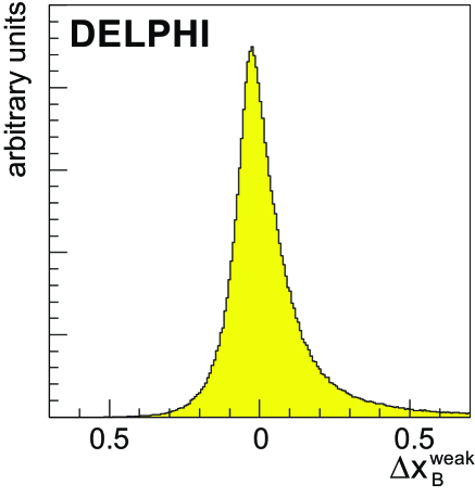
  Figure 1: Distribution of the precision of the NN estimator for $x^{\mathrm{w}eak}_{\mathrm{B}}$, defined as $\Delta x^{\mathrm{w}eak}_{\mathrm{B}}=(x^{\mathrm{w}eak}_{{\mathrm{B}},rec}-x^{\mathrm{w}eak}_{{\mathrm{B}},gen})/x^{\mathrm{w}eak}_{{\mathrm{B}},gen}$.

  4.1.4 The unfolding method

  The solution of Equation (5) for $f(x^{\mathrm{w}eak}_{\mathrm{B}})$ is a non-trivial problem since the solution can be highly oscillatory. A practical solution to this is provided by the Run (Regularised UNfolding) program [20] which applies regularisation techniques to impose the condition that the solution must be smooth. In practice, the algorithm defines a function $W(x^{\mathrm{w}eak}_{\mathrm{B}})$ used to provide a weight to the simulated distribution $g_{sim}(x^{\mathrm{w}eak}_{{\mathrm{B}},rec})$ such that it reproduces the data distribution $g(x^{\mathrm{w}eak}_{{\mathrm{B}},rec})$ as well as possible, i.e. $W(x^{\mathrm{w}eak}_{\mathrm{B}})$ is determined by a fit to the data. The result of the unfolding, up to a normalisation factor, is then given by

  $$f(x^{\mathrm{w}eak}_{\mathrm{B}}) = W(x^{\mathrm{w}eak}_{\mathrm{B}})\cdot f_{sim}(x^{\mathrm{w}eak}_{\mathrm{B}})$$ (6)

  where $f_{sim}(x^{\mathrm{w}eak}_{\mathrm{B}})$ is the fragmentation function used to generate the simulated events. By summing over bins in $x^{\mathrm{w}eak}_{\mathrm{B}}$, unfolded binned points are determined together with a complete covariance matrix.

  It is important to note that internally to Run, the weight factors are defined as a sum over orthogonal polynomials taken to be basis splines $P(x^{\mathrm{w}eak}_{\mathrm{B}})$,

  $$W(x^{\mathrm{w}eak}_{\mathrm{B}}) = \sum_{j=1}^{m}a_{j}\cdot P_{j}(x^{\mathrm{w}eak}_{\mathrm{B}})$$ (7)

  where $a_{j}$ are suitable expansion coefficients. Consequently, the difficult task of solving (5) reduces to deciding at which point to cutoff the sum in (7). This point, $j=m$, is referred to in what follows as the number of degrees of freedom of the unfolding procedure. Full details of the unfolding method can be found in reference [21].

  

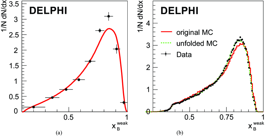
  Figure 2: a The result of unfolding $x^{\mathrm{w}eak}_{\mathrm{B}}$ from real data (points), and the generator-level $f_{sim}(x^{\mathrm{w}eak}_{\mathrm{B}})$ distribution, before applying weights (curve). b Distribution of $x^{\mathrm{w}eak}_{\mathrm{B}}$ in the data, $g(x^{\mathrm{w}eak}_{{\mathrm{B}},rec})$, compared to both the default simulation $g_{sim}(x^{\mathrm{w}eak}_{{\mathrm{B}},rec})$ and the simulation weighted for the results of the fragmentation function unfolding result shown in a.

  4.1.5 Unfolding results

  The result of the unfolding applied to the real data set is displayed in Figure 2a. The plot shows the unfolded, binned, data points together with an overlay of the ‘truth’ or generated $f(x^{\mathrm{w}eak}_{\mathrm{B}})$ distribution that is the input to the detector simulation. The binning of the unfolded points was chosen to match the observed resolution in $x^{\mathrm{w}eak}_{\mathrm{B}}$ according to the measurement uncertainties described in Section 4.1.3. For the case of $x^{\mathrm{w}eak}_{\mathrm{B}}$ the median (relative) error varied from about $5\%$ at an $x^{\mathrm{w}eak}_{\mathrm{B}}$ value close to $1.0$ and degraded to about $65\%$ at $x^{\mathrm{w}eak}_{\mathrm{B}}=0.2$. The number of degrees of freedom in the unfolding procedure was chosen to be as low as possible (i.e. five) in order to ensure a smooth result. The lower limit is constrained by the need to include all terms in the summation (7) for which the size of the expansion coefficients $a_{j}$ are significant.

  The results show that there is a basic disagreement in shape between the distribution unfolded from data and the corresponding truth distribution from the simulation before the application of weights. Figure 2b shows the excellent agreement that exists between data and simulation after appropriately weighting the generator distribution to agree with the result of the unfolding.

  In order to quantify the shape of the unfolded distribution, the mean ($\langle x\rangle=\int_{0}^{1}xf(x)dx$) and variance ($\sigma^{2}(x)=\int_{0}^{1}(x-\langle x\rangle)^{2}f(x)dx$) have been calculated and the results were: $\langle x^{\mathrm{w}eak}_{\mathrm{B}}\rangle=0.7140\pm 0.0007({\rm stat.})$ and $\sigma^{2}(x^{\mathrm{w}eak}_{\mathrm{B}})=0.0308\pm 0.0003({\rm stat.})$. The mean value quoted has been corrected to account for the effect of Initial State Radiation (ISR) which is necessary since $x$ is formed by scaling $E_{\mathrm{B}}^{\mathrm{w}eak}$ by the nominal beam energy of $45.6$ GeV. This is only strictly correct in the case of no ISR and in about $10\%$ of cases ISR reduces the energy available for the fragmenting b-quark system from the nominal value. The size of this effect on the analysis was evaluated from the simulation and the resulting mean value for $E_{\mathrm{B}}^{\mathrm{w}eak}$ was shifted by $+50$ MeV. The corresponding shift of $\langle x^{\mathrm{w}eak}_{\mathrm{B}}\rangle$ is $\delta\langle x^{\mathrm{w}eak}_{\mathrm{B}}\rangle=+0.0011$. The full bin-to-bin unfolding results including covariance matrices, are listed in Appendix B.

  4.1.6 Systematic uncertainties

  Systematic uncertainties on the unfolded distribution of $x^{\mathrm{w}eak}_{\mathrm{B}}$ have been evaluated from a wide variety of sources, the effects of which on $\langle x^{\mathrm{w}eak}_{\mathrm{B}}\rangle$ are presented in Table 2. In addition, statistical and systematic uncertainties for each of the nine unfolded bins of Figure 2a are given in Appendix B together with the associated covariance matrices.

  Technical systematics:

  Some crosschecks of the method were made on the simulation to ensure that the result of the unfolding was independent of the prior fragmentation function embedded in the simulation. In addition, an investigation was made of the sensitivity to the following technical aspects of the Run unfolding procedure:

  • The number of degrees of freedom, defined in Section 4.1.4, was increased from five (default value) to seven. The change in the results seen was then assigned as a systematic uncertainty to account for the degree of uncertainty present in determining at which point to terminate the summation described in Equation (7).

  • The number of knots in the basis spline representation of the weight $W(x^{\mathrm{w}eak}_{\mathrm{B}})$ (defined in Equation (7)) was varied and found to have a negligible effect on the results.

  • The binning of the reconstructed variable, $g(x^{\mathrm{w}eak}_{{\mathrm{B}},rec})$ in Equation (5), should be well matched to the resolution achieved in order to use the information optimally. A wide range of different binnings around the default choice was investigated and the results found to be consistent within the total systematic uncertainties quoted. Also, no improvement on the statistical precision was found.

  Selection cuts and background dependence:

  The hemisphere selection described in Section 4.1.2, includes selection cuts for ${\mathrm{b}\overline{b}}$ event enhancement and on the reconstructed scaled hemisphere energy $E_{hem}/E_{beam}$, both of which could potentially have an effect on the analysis if not accurately modelled in the simulation. The DELPHI b-tagging is based on impact parameter measurements which degrade at low momenta due to the increased effects of multiple scattering. This effect correlates the b-tagging information to the B-energy. Any variation in the unfolding result was checked when scanned over a wide range of b-tagging selection cuts i.e. different ${\mathrm{b}\overline{b}}$ purities. The results were found to be stable around the working point of ${\mathrm{b}\overline{b}}$ purity $\approx$ 96%. In addition, the effect of scanning around the nominal selection cut value of $E_{hem}/E_{beam}=0.5$ was investigated and the results found to be stable. No explicit systematic was assigned due to these two analysis selection cuts.

  Uncertainties in the size and composition of the background, i.e. $b(x^{\mathrm{w}eak}_{{\mathrm{B}},rec})$ in Equation (5), were also evaluated. Approximately 75% of the background was from non-${\mathrm{b}\overline{b}}$ events, primarily ${\rm c\overline{c}}$ events, which was accounted for as one of the b-physics modelling weights described later. The remainder was composed of cases where both b-quarks were found in the same hemisphere which occasionally happens e.g. in three-jet events or when a gluon splits into two b-quarks leaving a topology with four b-quarks in the initial state. In these cases, which occur in about $2\%$ of all hemispheres, the connection between the generated b-hadron energy and the reconstructed quantity becomes confused and hence were assigned to the background. It is assumed that the overall jet rate is well modelled in the simulation but the gluon splitting rate to ${\mathrm{b}\overline{b}}$ is varied, from the default value of $0.5\%$ by $\pm 50\%$ [22], and the change seen in the unfolding result is recorded as a systematic uncertainty.

  Reconstructed energy:

  The relationship between the reconstructed variable distribution in the simulation, $g_{sim}(x^{\mathrm{w}eak}_{{\mathrm{B}},rec})$, and the underlying physics p.d.f., $f_{sim}(x^{\mathrm{w}eak}_{\mathrm{B}})$, is

  $$g_{sim}(x^{\mathrm{w}eak}_{{\mathrm{B}},rec})=\int R(x^{\mathrm{w}eak}_{{\mathrm{B}},rec};x^{\mathrm{w}eak}_{\mathrm{B}})f_{sim}(x^{\mathrm{w}eak}_{\mathrm{B}})dx^{\mathrm{w}eak}_{\mathrm{B}}~{},$$ (8)

  where $R(x^{\mathrm{w}eak}_{{\mathrm{B}},rec};x^{\mathrm{w}eak}_{\mathrm{B}})$ is the response function defined in Equation (5). The unfolding is, by construction, insensitive to details of the prior fragmentation function $f_{sim}(x^{\mathrm{w}eak}_{\mathrm{B}})$ but only under the assumption that the response function, as derived from the simulation, is correct. It is therefore crucial that $R(x^{\mathrm{w}eak}_{{\mathrm{B}},rec};x^{\mathrm{w}eak}_{\mathrm{B}})$ be as close to the situation in the data as possible. Separate uncertainty contributions were assigned for each of the three corrections, described in Section 4.1.3, that affect directly modelling of the B-energy scale. Half of the full change in the result was taken as an uncertainty when: (a) the shifting/smearing procedure was turned off, (b) the spread of the multiplicity weights of about $1.0$ was changed by $\pm 50\%$ and (c) the hemisphere energy weight was switched off.

  Since the multiplicity tuning was dependent on a specific selection cut on the TrackNet variable around the $0.5$ point, it was checked that the results were not a strong function of this choice. The multiplicity weights were recalculated based on considering three regions in the TrackNet variable i.e. TrackNet$<0.2$, $0.2<$TrackNet$<0.8$ and TrackNet$>0.8$ and the analysis repeated. The results were found to be consistent to well within the quoted systematic uncertainties and no additional uncertainty was assigned.

  A further crosscheck was made by using a different choice for $E_{\mathrm{B}}^{\mathrm{w}eak}$ other than the Bayesian neural network variable described in Section 4.1.3. For this test, $E_{\mathrm{B}}^{\mathrm{w}eak}$ was estimated by applying a rapidity algorithm (described in Appendix A) and corrected for missing neutral energy based on a parameterisation from the simulation. A detailed description of this correction is given elsewhere [23]. Repeating the analysis, the change seen in the result for $x^{\mathrm{w}eak}_{\mathrm{B}}$ was -0.0011, well contained within the assigned total systematic uncertainty.

  uncertainty class	item	$\delta\langle x^{\mathrm{w}eak}_{\mathrm{B}}\rangle$
  technical	number of degrees of freedom	$+0.0025$
  selection cuts and backg. dependence	${\rm g\to b\overline{b}}$	$+0.0004$
  reconstructed energy	neutral energy smearing	$~{}~{}0.0023$
  	fragmentation track multiplicity	$+0.0030$
  	b-decay track multiplicity	$-0.0004$
  	neutral multiplicity	$+0.0010$
  	hemisphere scaled energy $E_{hem}/E_{beam}$	$~{}~{}0.0003$
  b-physics modelling	b-hadron lifetimes	$-0.0004$
  	b-hadron production fractions	$~{}~{}0.0002$
  	hemisphere quality	$-0.0018$
  	$\mbox{B}^{\ast\ast}$ rate	$-0.0018$
  	$\mbox{B}^{\ast\ast}$ $Q$-value dependence	$~{}~{}0.0003$
  	$\rm K^{0}$ rate	$+0.0005$
  	$\mbox{B}^{\ast}$ rate	$-0.0001$
  	semileptonic decay rate	$-0.0001$
  	wrong sign charm rate	$+0.0001$
  	c- and b-quark efficiency	$~{}~{}0.0001$
  calibration stability & simulation statistics	calibration periods	$~{}~{}0.0025$
  	finite simulation statistics	$~{}~{}0.0005$
  Total		$~{}~{}0.0060$

  Table 2: Systematic uncertainty on the mean value of the unfolded $x^{\mathrm{w}eak}_{\mathrm{B}}$ distribution. The total is the sum in quadrature of all contributions. The sign indicates the correlation between the change in an uncertainty source and the shift in the final result. Uncertainties assigned by turning a weight on/off have no sign.

  b-physics modelling:

  The remaining systematic contributions concern quantities for which the simulation was weighted in order to account for known discrepancies with the data. Weights were constructed to change the lifetimes and production fractions of the b-hadron species to more recent world average values [6]:

  $\tau(\rm B^{+})=1.638\pm 0.011$ ps,	$f(\rm B^{+})=(39.9\pm 1.1)$%
  $\tau(\rm B_{\rm d}^{0})=1.530\pm 0.009$ ps,	$f(\rm B_{\rm d}^{0})=(39.9\pm 1.1)$%
  $\tau(\rm B_{\rm s}^{0})=1.470\pm 0.027$ ps,	$f(\rm B_{\rm s}^{0})=(11.0\pm 1.2)$%
  $\tau({\mathrm{b}-baryon})=1.383\pm 0.049$ ps,	$f({\mathrm{b}-baryon})=(9.2\pm 1.9)$% .

  Systematic uncertainties from these sources were based on varying them within the quoted one standard deviation uncertainties for the case of the lifetimes and by switching the weights on/off for the case of the production fractions. The ‘hemisphere quality’ was a quantity flagging the presence of potentially badly reconstructed tracks in the hemisphere. Improved agreement with the data was achieved in many reconstructed quantities by weighting the hemisphere quality distribution in the simulation to agree with that seen in data. The change induced by varying the spread of the weight around $1.0$ by $\pm 50\%$ from the nominal value was assigned as a systematic uncertainty.

  By default the production rate of excited $\mbox{B}^{\ast\ast}$ states was adjusted in the simulation to be $25\%$ per ${\rm B}$ meson hemispheres. This rate was then varied from $15\%$ to $35\%$ and half the total change seen in the results, assigned as a systematic. In addition, sensitivity to the $\mbox{B}^{\ast\ast}$ $Q$-value was tested by applying a weight to force the simulated $Q$-value distribution to be that suggested by a previous DELPHI analysis [24], and the change in the results was assigned as a systematic uncertainty.

  Systematic uncertainties from the $\mbox{B}^{\ast}$ rate, ${\rm K^{0}_{S}}$ rate and the b-hadron semi-leptonic branching fraction were accounted for by changing their values in the simulation by the same relative uncertainty quoted on current world averages [6]. In addition an uncertainty was assigned due to changing the ‘wrong-sign’ ${\rm D_{s}}$ production rate, i.e. ${\rm D_{s}}$ production from ${\rm W}^{-}\rightarrow\overline{c}s$ decay, by $100\%$.

  Finally a weight was applied to the simulation based on the results of a double hemisphere tagging analysis in order to correct the efficiency to tag $\rm Z\to\rm c\overline{\rm c}$ events and $\rm Z\to\rm b\overline{\rm b}$ events to that measured from the data. At the analysis working point of ${\mathrm{b}\overline{b}}$ purity of $96\%$, the correction to the b efficiency was about $-2\%$ and the correction to the c efficiency about $-12\%$. A systematic from this source was assigned to be the full difference in the results when this weight was removed.

  Calibration stability and simulation statistics:

  A spread is observed in the results as a function of time slices dividing up the data. The likely source of this effect is the division of the period into different calibration periods of the vertex detector and half of the full spread in results has been assigned as a systematic uncertainty. The effect of having finite simulation statistics for the determination of the transfer matrix was small and was evaluated by varying the elements of the matrix up and down by one statistical standard deviation.

  4.2 The weighted fitting analysis

  The procedures used for b-hadron energy reconstruction and measurement of the b-hadron fragmentation distribution are different from those applied in the previous approach. The B hadron energy is obtained by subtracting the energy taken by fragmentation tracks from the reconstructed energy of the jet containing the B candidate. The b-hadron fragmentation distribution is determined by fitting a weight distribution on simulated events such that the corresponding reconstructed B energy distribution agrees with the one measured using real data events.

  4.2.1 Hadronic event selection

  Hadronic ${\rm Z}$ decays were selected using the following requirements:

  • $|\cos{(\theta_{thrust})}|<0.95$;

  • at least 15 particles, charged and neutrals, reconstructed.

  Charged particles from b-hadron decays can be identified from other charged hadrons using their positive impact parameter measured relative to the event main vertex. For a hadronic event resulting from the hadronisation of light quarks, charged particle impact parameters are expected to be compatible with the beam interaction position. A variable, $P_{\rm btag}$, has been used, which has a flat distribution for such events and which is peaked at low values for events containing heavy quarks whose decay generates charged particles with offsets [14]. In Table 3 are given the fraction of selected events in data and simulation, the expected fraction of non-$\mathrm{b}\overline{b}$ events and the efficiency for $\mathrm{b}\overline{b}$ events. According to these values, samples of hadronic events containing about 10$\%$ contamination from non-$\mathrm{b}\overline{b}$ events can be isolated with an efficiency higher than 60$\%$ for those originating from b-quarks. Remaining differences between real and simulated events have been included in the evaluation of systematics.

  selection on $P_{\rm btag}$	$<10^{-3}$	$<10^{-4}$	$<10^{-5}$	$<10^{-6}$	$<10^{-8}$	$<10^{-10}$
  Data: fraction of
  selected events ($\%$)	17.6	14.3	11.8	9.9	6.8	4.5
  MC: fraction of
  selected events ($\%$)	17.2	14.0	11.5	9.5	6.4	4.2
  MC: b-purity ($\%$)	88.7	93.5	96.1	97.6	99.0	99.9
  MC: b-efficiency ($\%$)	69.4	59.3	50.1	41.9	28.6	19.1

  Table 3: Variation of the selected event sample composition and efficiency for $\mathrm{b}\overline{b}$ events versus the selection cut on the $P_{\rm btag}$-variable.

  In the following, samples of hadronic events depleted in b flavour have been selected by a selection cut on the b-tagging probability ($P_{\rm btag}\geq$ 10 $\%$) evaluated for the whole event, whereas b-enriched samples have been retained using $P_{\rm btag}\leq 10^{-3}$.

  4.2.2 b-hadron energy reconstruction

  The b-hadron energy is determined in two steps. Jets are firstly reconstructed and their energies are obtained from a constrained fit requiring energy-momentum conservation for the whole event. Then, considering only those jets for which the axis is inside the VD acceptance ($\left|\cos{\theta_{jet}}\right|<0.75$), particles are classified as B decay products or fragmentation particles. For charged particles, their offsets relative to the event main vertex, and their rapidity measured relative to the jet axis are used in this classification, whereas for neutrals only the rapidity is used.

  Differences between real and simulated events can originate from a behaviour of the detector that differs from its expected performances or from different particle production characteristics in the events. As the reconstruction accuracy for charged particles depends on the type of sub-detectors used and as differences remain between the fractions of sub-detectors involved in the data and in the simulation, corrections have been applied. The procedure, equivalent to the removal of a sub-detector, consists in rescaling the values of measurement uncertainties and in smearing the corresponding track parameter values. These corrections, which apply to about $4\%$ of all charged particles, depend on the type of the removed sub-detector and were determined using the simulation, by comparing uncertainty matrix elements for tracks with and without the corresponding sub-detector involved. In addition, as the mass distribution of reconstructed weakly decaying particles (such as those corresponding to the ${\rm D}^{0}$ or ${\rm D}^{+}$ mesons) has a width which is larger in real data by about $20~{}\%$, a smearing corresponding to the same fraction of their measurement uncertainty has been applied to simulated tracks.

  After these corrections individual particle momentum distributions have been compared in real and simulated events. These distributions considered separately for b-depleted and b-enriched samples have been normalised using the respective number of selected hadronic events in each category. To match corresponding data/simulation distributions a momentum dependent correction is then applied, which consists in removing tracks alternatively in data or in the simulation depending if the measured ratio is larger or lower than unity. This correction has been determined separately for b-depleted and b-enriched samples and also, independently, for charged and neutral particles.

  To avoid a possible bias induced by a correlation between the assumed shape of the fragmentation function and the applied correction, the latter has been evaluated iteratively using as input in its determination the fragmentation distribution measured at the previous step. In practice one iteration was used, as the observed absolute variation between the second and first step on the resulting $\langle x^{\mathrm{w}eak}_{\mathrm{B}}\rangle$ value was of the order of $10^{-3}$.

  In a given event, jets are reconstructed using the Lund LUCLUS algorithm [25] with the $d_{\rm join}$ parameter (${\rm PARU}(44)$) value set to 5.0 GeV/$c$. A first evaluation of the jet energies is obtained using the jets directions, energies, masses and imposing total energy-momentum conservation for the whole event. If the missing energy in a jet is larger than 1 GeV, a 4-vector is added to the jet. Its direction is taken to be the same as the jet direction and the missing momentum is evaluated assuming that the missing particle mass is zero. Analysing simulated events, the relative uncertainty on the missing energy is measured to be 20$\%$, and uncertainties on angles of the missing particle are 50 mrad. Energy momentum conservation is then applied again to the whole event, and particle parameters (for charged, neutral and possibly missing) are fitted. After this procedure, 4-vectors of charged and neutral particles have been fitted, and possibly new 4-vectors corresponding to missing energy in each jet have been obtained. Jets are reevaluated ($p_{\mathrm{j}et}$) using this set of tracks and applying the same LUCLUS algorithm. Fractions of the fitted charged, neutral and missing energy are compared in Table 4. Relative differences are at the level of a few $10^{-3}$. A comparison between data and the simulation has been also made for the averages and variances of charged and neutral particle multiplicities. The results are given in Table 5.

  $\mathrm{b}\overline{b}$-depleted events
  Sample	$E_{ch.}~{}+~{}E_{neu.}$	$E_{ch.}$	$E_{neu.}$	$E_{miss.}$
  Data	$0.8644$	$0.5759$	$0.2879$	$0.1363$
  MC	$0.8676$	$0.5778$	$0.2893$	$0.1323$
  (Data-MC)/MC	$-0.0037$	$-0.0033$	$-0.0048$	$+0.030$
  $\mathrm{b}\overline{b}$-enriched events
  Sample	$E_{ch.}~{}+~{}E_{neu.}$	$E_{ch.}$	$E_{neu.}$	$E_{miss.}$
  Data	$0.8423$	$0.5891$	$0.2528$	$0.1589$
  MC	$0.8423$	$0.5885$	$0.2535$	$0.1579$
  (Data-MC)/MC	$0.0000$	$+0.0010$	$-0.0027$	$+0.0063$

  Table 4: Fitted fractions of charged energy $(E_{ch.})$, neutral energy $(E_{neu.})$ and their sum reconstructed in $\mathrm{b}\overline{b}$-depleted and $\mathrm{b}\overline{b}$-enriched event samples in data and simulation. The missing energy $(E_{miss.})$ fitted fraction is also given.

  $\mathrm{b}\overline{b}$-depleted events
  Sample	charged	neutrals
  Data	$22.93~{}(7.94)$	$10.47~{}(3.84)$
  MC	$22.96~{}(7.62)$	$10.56~{}(3.82)$
  $\mathrm{b}\overline{b}$-enriched events
  Sample	charged	neutrals
  Data	$25.34~{}(7.60)$	$10.95~{}(3.80)$
  MC default	$24.74~{}(7.45)$	$10.88~{}(3.82)$
  MC fitted	$25.16~{}(7.48)$	$10.96~{}(3.83)$

  Table 5: Charged and neutral particle multiplicities (variances) measured in data and simulation.

  

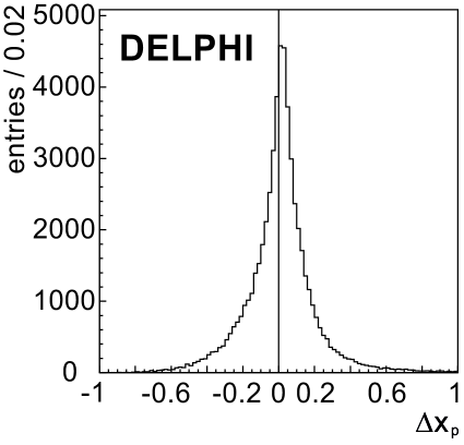
  (a)

  

  (b)

  Figure 3: a distribution of $\Delta x_{p}=(p^{rec.}_{\mathrm{B}}-p^{gen.}_{\mathrm{B}})/p^{gen.}_{\mathrm{B}}$ for weakly decaying b-hadrons. The full width at half maximum is equal to 16 $\%$. b acceptance for signal events versus $p_{\mathrm{B}}^{\mathrm{w}eak}/p_{\mathrm{b}eam}$.

  Each jet pointing through the detector barrel region defined by $\left|\cos{\theta_{jet}}\right|<0.75$ is considered in turn, and charged particles belonging to the jet are used to reconstruct a B decay vertex candidate. It is then required that these tracks have at least two VD hits associated in $R\phi$ and a minimum positive impact parameter with significance larger than $\sqrt{3}\sigma$ relative to the main vertex of the event. A secondary vertex is then reconstructed. Tracks with a too large contribution to the $\chi^{2}$ are removed from the fit in an iterative way. For a candidate to be accepted, it is required that at least three tracks with the $Z$-coordinate measured in the VD remain, and that the distance between the secondary and the primary vertex projected along the jet direction is larger than 500 $\mu m$. The reconstructed mass must not exceed the B mass (all particles are assumed to be pions). If not, particles ordered by increasing values of their rapidity measured relative to the jet axis, are eliminated in turn. If the reconstructed mass is smaller than the B mass, particles belonging to the same jet ordered by decreasing rapidity values, are added in turn. For charged particles, offsets relative to the primary and secondary vertices are also examined. To possibly include a track, it is required that its offset relative to the secondary vertex is smaller than its offset relative to the primary vertex. The procedure is stopped when the mass of selected particles is closest to the B mass.

  The B momentum is obtained by subtracting from the fitted jet momentum the momentum of the tracks from the jet, which have not been assigned to the B candidate. For the candidate to be accepted, the sum of the jet neutral energy and of the charged energy for tracks that are simultaneously compatible with the primary and secondary vertices has to be smaller than 20 GeV. Figure 3a shows the difference between the reconstructed and the simulated B momentum, divided by the simulated value.

  According to the simulation the applied algorithm has an average efficiency for the signal of $19\%$ (see Figure 3b) and a contamination of $5\%$ from non-b jets. The efficiency is rather flat for $p_{\mathrm{B}}^{\mathrm{w}eak}/p_{\mathrm{b}eam}>0.5$ and is still 50$\%$ of its maximum value around $p_{\mathrm{B}}^{\mathrm{w}eak}/p_{\mathrm{b}eam}=0.3$. There are 134282 candidates selected in the data sample. The quoted efficiency for the signal differs from values given in Table 3, because the latter refers to the whole event whereas the former is for b-jets after applying the additional cuts used in the analysis.

  Measured $p_{\mathrm{B}}^{\mathrm{w}eak}/p_{\mathrm{b}eam}$ distributions are compared in Figure 4 with expectations from the simulation. The two distributions agree for $\mathrm{b}\overline{b}$-depleted events and show a marked difference for events in the b-enriched sample. In what follows, the transformation of the non-perturbative QCD distribution used in the simulation, required to make the weighted distribution of simulated events agree with the data, has been determined.

  

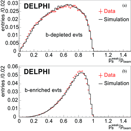
  Figure 4: Comparison between the measured distributions of the beam momentum fraction taken by a b-hadron, obtained in data (points with error bars) and in the ${\mathrm{q}\overline{q}}$ simulation (histogram). a Depleted b-sample. b Enriched b-sample. The distributions have been normalised to unity.

  4.2.3 Determination of the b-hadron fragmentation distribution

  The binned distribution of the reconstructed $p_{\mathrm{B}}^{\mathrm{w}eak}/p_{\mathrm{j}et}$ variable has been fitted by minimising a $\chi^{2}$, which includes effects from the data and simulation statistics and from the weighting procedure.

  In each bin the number of measured events is compared with an estimated number obtained in the following way:

  • contributions from background events are taken from the ${\mathrm{q}}\overline{\mathrm{q}}$ simulation. They comprise three components: non-b jets in non-$\mathrm{b}\overline{b}$ events, non-b jets in $\mathrm{b}\overline{b}$ events and b jets from gluon splitting. In simulated events, the fractions of these components are respectively equal to $5.2\%,~{}0.45\%~{}{\rm and}~{}0.24\%$ of the analysed events. The number of gluon splitting candidates has been multiplied by 1.5 to account for its measured rate at LEP [22].

    

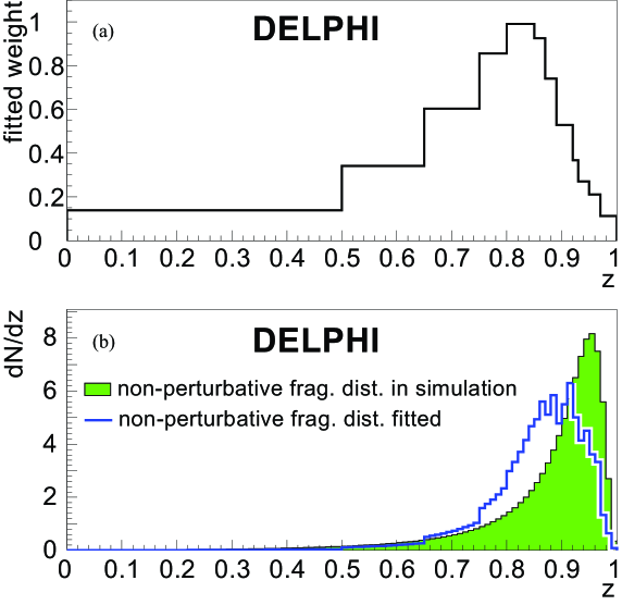
    Figure 5: Fitted $z$ distribution on data selected events. a Distribution of the fitted weights. b Comparison between the initial Peterson distribution used in the simulation generator (shaded), and the corresponding distribution favoured by data events (solid line). The visible steps on this last distribution correspond to the applied weights, which have constant values over each bin as illustrated in a.

  • The distribution of signal events is obtained by weighting $\mathrm{b}\overline{b}$ simulated events. This weight contains several components, which have been determined to correct the values of parameters used in the simulation so that they agree with corresponding measured quantities as: ${\rm B}$ lifetimes, ${\rm B}$ charged particle multiplicity and ${\rm B}^{**}$ fraction in jets. The used values of these measured quantities are the same as those used in the regularized unfolding analysis, as detailed in Section 4.1.6.

  • A weight, whose parameters are fitted, is also applied for each value of the simulated $z$ variable (see Section 2). The weights are constant over intervals in $z$ (the weight function is a histogram with a non-uniform binning).

  • The normalisation of $\mathrm{b}\overline{b}$ events is taken as a free parameter.

  To prevent oscillations between the contents of nearby bins of the weight histogram, a regularisation term is included in the $\chi^{2}$:

  $$\chi^{2}_{\rm reg}=C\times\left[2\times n(i)-n(i-1)-n(i+1)\right]^{2}~{},$$ (9)

  where $C$ is a parameter whose value ($C=1$) has been determined empirically using simulated events; and $n(i)$ is the content of bin $i$.

  Distributions corrected for all effects are then obtained using corresponding generated distributions from simulated events before any selection criteria, and by applying the weight distribution fitted on real events, which depends on the $z$ variable generated value for each simulated b-hadron. Statistical uncertainties in each bin, of these distributions, have been obtained using the full covariance matrix of the fitted parameters and generating toy experiments.

  The fitted weight distribution obtained with the data sample is given in Figure 5. This figure shows also the $z$ distribution as favoured by the data. It is rather different from the Peterson distribution which was used in the simulation, and shown on the same figure.

  As in the companion analysis described in Section 4.1, the differential b-quark fragmentation distribution is evaluated in nine intervals of the $x^{\mathrm{w}eak}_{\mathrm{B}}$ variable whose averaged value is equal to $\langle x^{\mathrm{w}eak}_{\mathrm{B}}\rangle=0.6978\pm 0.0010$. It is displayed in Fig. 6. Measured values of the distribution in each bin and the corresponding statistical error matrix are given in Appendix C. Its integral has been normalised to unity.

  4.2.4 Systematic uncertainties

  Systematic uncertainties have been evaluated for each value of the fragmentation distribution obtained in the nine $x^{\mathrm{w}eak}_{\mathrm{B}}$ intervals. In Table 6, systematics on $\langle x^{\mathrm{w}eak}_{\mathrm{B}}\rangle$ have been reported. Sources of systematic uncertainties have been ordered as in the previous analysis (Section 4.1.6).

  Technical systematics:

  The weight function consists of twelve bins in $z$ whose content is fitted. Choices for the bin definition and bin number can induce a systematic uncertainty on the extracted distribution. This has been studied by comparing the generated and fitted distributions in simulated events. Generated events correspond to the average value $\langle x^{\mathrm{w}eak}_{\mathrm{B}}\rangle_{gen.}^{sim.}=0.7057$ and have been reconstructed at $\langle x^{\mathrm{w}eak}_{\mathrm{B}}\rangle_{rec.}^{sim.}=0.7060$. The quoted values have been corrected for the effect of the beam radiation which corresponds to an increase of $0.0015$. The observed difference on $\langle x^{\mathrm{w}eak}_{\mathrm{B}}\rangle$ is equal to $+0.0003$.

  These results depend also on the choice for the value of the curvature parameter $C$ introduced in the $\chi^{2}$ expression (see Equation (9)). Changing the value of this parameter between $0.02$ and $5.0$ gives variations on $\langle x^{\mathrm{w}eak}_{\mathrm{B}}\rangle$ at the level of $\pm 0.002$ on simulated events and even smaller values on real data events. In the following analysis the value $C=1$ has been used and effects of the variation of this parameter between $0.02$ and $5.0$ are included in the evaluation of systematic uncertainties.

  Selection cuts and background dependence:

  In the analysed sample with the selection $P_{\rm btag}\leq 10^{-3}$, the estimated fraction of non-b candidates amounts to $5.2\%$. In Table 3 it was observed that the fraction of selected events is a few $\%$ (relative) higher in real data. As this effect remains in samples of high purity in $\mathrm{b}\overline{b}$ events, its main origin comes most probably from a difference in efficiency between real and simulated $\mathrm{b}\overline{b}$ events. A possible underestimate of the selection efficiency to non-$\mathrm{b}\overline{b}$ events in the simulation amounts then to $10\%$ (relative) at maximum. The effect of a $\pm 20\%$ variation on the non-b background level has been evaluated; it gives $\delta\langle x^{\mathrm{w}eak}_{\mathrm{B}}\rangle=\pm 0.0012$.

  The stability of the measured $x^{\mathrm{w}eak}_{\mathrm{B}}$ distribution has been studied for different selections on the value of the $P_{\rm btag}$ variable. The resulting $\langle x^{\mathrm{w}eak}_{\mathrm{B}}\rangle$ is stable within $\pm 0.001$. For the corresponding systematic evaluation, half the difference obtained using selection cuts at $10^{-4}$ and $10^{-10}$ has been used.

  Hadronic jets have been reconstructed using the LUCLUS algorithm with the value of the parameter defining the jets, $d_{\rm join}$=5 GeV/$c$. Sensitivity of present results on the value of this parameter has been studied by redoing the measurements using $d_{\rm join}$=10 GeV/$c$. The variation on $\langle x^{\mathrm{w}eak}_{\mathrm{B}}\rangle$ is equal to $+0.0002$.

  In a jet, there are charged particles which can be compatible simultaneously with the primary and the secondary vertex. Concerning neutral particles, the angular resolution does not allow them to be attached with confidence to one of the two vertices. The energy taken by these two classes of tracks is denoted “ambiguous” energy. In the analysis, events have been selected requiring that the “ambiguous” energy is lower than $20$ GeV. The stability of the results has been studied by changing the value for this selection criterion. A change from $20$ GeV to 15 GeV results in a $25\%$ decrease in the number of selected events, and no variation is measured for $\langle x^{\mathrm{w}eak}_{\mathrm{B}}\rangle$. A change from $15$ GeV to $10$ GeV keeps $50\%$ of the initial statistics. The corresponding variation is taken as a systematic uncertainty, which corresponds to a variation of $\langle x^{\mathrm{w}eak}_{\mathrm{B}}\rangle$ by $-0.0034$.

  Events have been selected requiring at least three charged particles at the candidate B decay vertex. Taking the difference observed for selections with at least three and five charged particles as an evaluation for the corresponding systematic, the variation on $\langle x^{\mathrm{w}eak}_{\mathrm{B}}\rangle$ is equal to $+0.0012$.

  The rate for b-hadron production originating from gluon coupling to $\mathrm{b}\overline{b}$ pairs has been measured by LEP experiments and found to be larger than the rate used in the simulation by a factor $1.5$. The corresponding systematic uncertainty has been evaluated, considering the uncertainty, of $30\%$, obtained by DELPHI on this quantity [26]. The variation on $\langle x^{\mathrm{w}eak}_{\mathrm{B}}\rangle$ is equal to $-0.0001$.

  Reconstructed energy:

  The analysis uses the beam energy as a constraint in a global fit of 4-momenta of charged and neutral particles, such that the total energy and momentum of the event is conserved.

  Corrections applied on charged and neutral energy distributions have been described in Section 4.2.2. They induce a variation on $\langle x^{\mathrm{w}eak}_{\mathrm{B}}\rangle$ of $+0.0017$. The corresponding systematic uncertainty has been evaluated taking the effect of this correction.

  Measured jet multiplicities are not identical in data and in simulated events. Taking as reference the fraction of two-jet events, fractions of three- and four-jet events have to be corrected respectively by $-5\%$ and $+13\%$ in the simulation. Simulated events have been weighted accordingly so that the two distributions agree. From the statistical accuracy of this correction, the systematic uncertainty has been evaluated to be one third of the correction. This corresponds to $\delta\langle x^{\mathrm{w}eak}_{\mathrm{B}}\rangle=-0.0001$.

  uncertainty class	item	$\delta\langle x^{\mathrm{w}eak}_{\mathrm{B}}\rangle$
  technical	fitted function shape	$~{}0.0015$
  	curvature parameter in $\chi^{2}$	$~{}0.0020$
  selection cuts and backg. dependence	b-tagging selection cut	$~{}0.0010$
  	non-b background level	$~{}0.0012$
  	jet clustering parameter value	$~{}0.0002$
  	ambiguous energy level	$~{}0.0034$
  	secondary vertex multiplicity	$~{}0.0012$
  	$\mathrm{g}\to b\overline{b}$	$-0.0001$
  reconstructed energy	corrections on tracks	$~{}0.0017$
  	jet multiplicity	$-0.0001$
  b-physics modelling	b-hadron lifetimes	$-0.0005$
  	$\mathrm{B}^{**}$ rate	$-0.0008$
  	b-decay track multiplicity	$-0.0008$
  calibration stability	calibration periods	$~{}0.0038$
  Total		$~{}0.0064$

  Table 6: Systematic uncertainty on the mean value of the $x^{\mathrm{w}eak}_{\mathrm{B}}$ distribution in the weighted fitting analysis. The total is the sum in quadrature of all contributions. The sign indicates the correlation between the change in an uncertainty source and the shift in the final result. Uncertainties assigned by turning a weight on/off have no sign.

  b-physics modelling:

  Variations of the values of parameters that govern decay properties or production characteristics of b-hadrons have been also considered.

  Simulated events have been generated using the same lifetime value of $\tau_{\mathrm{B}}=1.6~{}ps$. Events have been weighted such that each type of b-hadron is distributed according to its corresponding lifetime, as given in reference [6]. Taking, as systematics, the total variation induced by this correction, the variation on $\langle x^{\mathrm{w}eak}_{\mathrm{B}}\rangle$ is equal to $-0.0005$.

  In the simulation, the $\mbox{B}^{\ast\ast}$ production rate in a b-quark jet amounts to $32\%$. A weight is applied on b-hadrons which originate from $\mbox{B}^{\ast\ast}$ decays to lower the effective $\mbox{B}^{\ast\ast}$ rate to $25\%$. The corresponding systematic has been taken as the variation on $\langle x^{\mathrm{w}eak}_{\mathrm{B}}\rangle$, namely $-0.0008$.

  The difference between simulated, $n_{ch}^{sim.}({\mathrm{B}})$, and measured, $n_{ch}^{meas.}({\mathrm{B}})$, average charged multiplicities in b-hadron decays amounts to $0.06$:

  $$n_{ch}^{meas.}({\mathrm{B}})=4.97\pm 0.03\pm 0.06,~{}n_{ch}^{sim.}({\mathrm{B}})=4.91.$$ (10)

  This difference has been corrected by weighting events using a weight that has a linear variation with the actual b-hadron charged multiplicity in a given event. The simulated multiplicity distribution has been fitted with a Gaussian of standard deviation $(\sigma_{nch})$ equal to $2.03$ charged particles. Probability values, for a given charged multiplicity $i,~{}P_{i},$ have been transformed into:

  $$P_{i}^{T}=P_{i}\left[1+\beta(n_{ch}^{sim.}-i)\right]~{}.$$ (11)

  The value of $\beta$ is obtained by requiring that the new average multiplicity computed using $P_{i}^{T}$ is equal to $n_{ch}^{meas.}(B)$. Then:

  $$\beta=\frac{n_{ch}^{sim.}-n_{ch}^{meas.}}{\sigma_{nch}^{2}}~{}.$$ (12)

  The corresponding systematic uncertainty has been evaluated by considering an uncertainty of $\pm 0.1$ charged particles on $n_{ch}^{meas.}$. The variation on $\langle x^{\mathrm{w}eak}_{\mathrm{B}}\rangle$ is equal to $\mp 0.0008$.

  Calibration stability and simulation statistics:

  The stability of the energy calibration has been studied dividing the analysed data samples in five time ordered subsamples of similar statistics. The statistical accuracy of each $\langle x^{\mathrm{w}eak}_{\mathrm{B}}\rangle$ measurement is of about $0.002$. The systematic uncertainty attached to the energy reconstruction has been evaluated by taking half the difference between the two extremes of the five measurements of $\langle x^{\mathrm{w}eak}_{\mathrm{B}}\rangle$: $\pm 0.0038$.

  Uncertainties corresponding to the finite statistics of simulated events have been included in the statistical uncertainty of the measurements.

  4.3 Combination of the $x^{\mathrm{w}eak}_{\mathrm{B}}$ distributions

  The results of the two $x^{\mathrm{w}eak}_{\mathrm{B}}$ measurements obtained in Sections 4.1 and 4.2 have been averaged. In this combination a complete correlation has been assumed between statistical uncertainties, due to the common data used by the two analyses. The following sources of systematic uncertainties have been considered also as fully correlated:

  • neutral energy smearing in the regularised unfolding analysis with ambiguous energy level in the weighted fitting analysis;

  • $g\rightarrow b\overline{b}$ branching fraction;

  • $\mbox{B}^{\ast\ast}$ production rate;

  • b-hadron lifetimes;

  • b-decay track multiplicity;

  • b-hadron production fractions;

  • wrong sign charm rate.

  bin	value	statistical	systematic	$\sqrt{\sigma_{stat}^{2}+\sigma_{syst}^{2}}$
  borders		uncertainty	uncertainty
  0.10 – 0.30	0.194	0.004	0.020	0.020
  0.30 – 0.42	0.474	0.008	0.031	0.032
  0.42 – 0.54	0.734	0.009	0.037	0.038
  0.54 – 0.64	1.112	0.013	0.048	0.050
  0.64 – 0.73	1.753	0.021	0.057	0.060
  0.73 – 0.80	2.641	0.029	0.064	0.070
  0.80 – 0.88	3.013	0.029	0.119	0.122
  0.88 – 0.94	1.787	0.028	0.119	0.122
  0.94 – 1.00	0.227	0.015	0.046	0.049

  Table 7: The combined unfolded and weighted results, per bin, for $f(x^{\mathrm{w}eak}_{\mathrm{B}})$. Quoted uncertainties have been scaled by $1.31$.

  

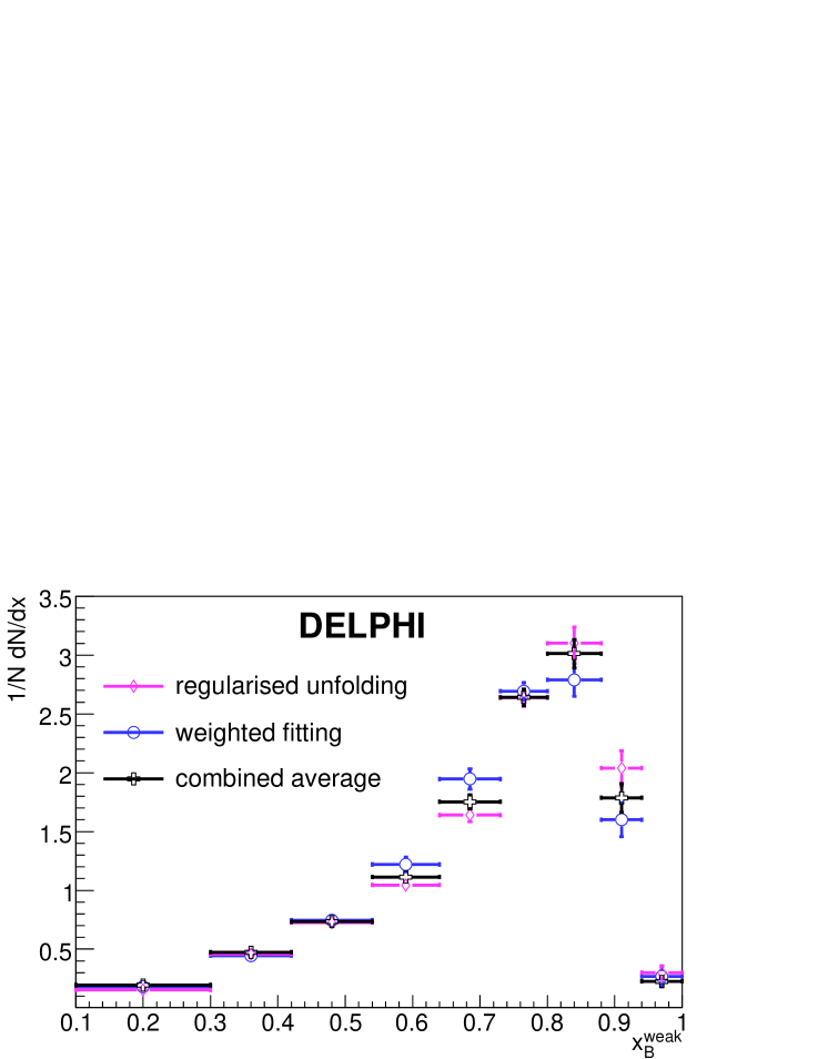
  Figure 6: Measured fragmentation distributions in the two analyses and their combined average. Uncertainties on the combined average are scaled by $1.31$.

  Other systematic uncertainties, some of them large, have been taken as uncorrelated as the two analyses are using different techniques. No significant correlation was observed between the two measurements when considering event samples recorded during the same time periods.

  The combined $x^{\mathrm{w}eak}_{\mathrm{B}}$ distribution has been obtained by a fit using the full error matrix of the two analyses. This matrix has two insignificant eigenvalues which have been removed. The fit has therefore $7$ degrees of freedom and the $\chi^{2}$ value is $11.96$ (probability of $10.2\%$).

  The combined value of the $f(x^{\mathrm{w}eak}_{\mathrm{B}})$ distribution in each bin is given in Table 7 and in Figure 6. The corresponding statistical and total error matrices are given in Appendix D. In the following, all the quoted uncertainties on the $f(x^{\mathrm{w}eak}_{\mathrm{B}})$ distribution bins are scaled by $1.31$. This corresponds to $\chi^{2}/\mbox{NDF}=1$. By rescaling the uncertainties it is ensured that possible poor fit probabilities of models with the combined measurement do not originate from an underestimate of quoted measurement uncertainties. The average value of this distribution is equal to:

  $$\langle x^{\mathrm{w}eak}_{\mathrm{B}}\rangle=0.699\pm 0.011~{}.$$ (13)

  This value is largely influenced by correlations between the $x^{\mathrm{w}eak}_{\mathrm{B}}$ distributions from the two analyses.

  The combined result is compared with model predictions in Section 4.4 and with other experimental results from ALEPH [27], OPAL [28] and SLD [29] at the ${\rm Z}$ pole in Section 6.

  4.4 Fits to hadronisation models

  The measured $f(x^{\mathrm{w}eak}_{\mathrm{B}})$ distribution has been compared to functional forms that are in common use inside event generators. Since the Lund [30], Lund-Bowler [31] and Peterson [18] models are functions of $z$ and, in the case of Lund and Lund-Bowler, of a transverse mass variable $m_{{\mathrm{b}}\bot}^{2}$ that varies event-to-event, these functions cannot simply be fitted to the unfolded distributions. Instead, parameters of these models have been fitted to data using a high statistics Monte-Carlo sample at the generator level by applying weights. The configuration of the event generator used for these studies is as given in Table 8. For further details see reference [17].

  Event Generator	JETSET/PYTHIA 6.156
  Perturbative ansatz	Parton shower ($\Lambda_{QCD}=0.297$ GeV, $Q_{0}=1.56$ GeV)
  Non-perturbative ansatz	String fragmentation
  Fragmentation function	Peterson with $\epsilon_{\mathrm{b}}=0.004$
  Bose-Einstein correlations	Disabled

  Table 8: Details of the event generator used together with some of the more relevant parameter values that have been tuned to the DELPHI data.

  For each event in the generated sample, the values of the internal variables $z$ and $m_{\mathrm{b}\perp}^{2}$ are used to define a weight $w=f_{\rm fit}(z,m_{\mathrm{b}\perp}^{2};\vec{X}_{\rm fit})/f_{\rm Peterson}(z;\epsilon_{\mathrm{b}})$, where $f_{\rm fit}(z,m_{\mathrm{b}\perp}^{2};\vec{X}_{\rm fit})$ stands for the Lund, Lund-Bowler or Peterson fitted distributions, $\vec{X}_{\rm fit}$ to their corresponding parameters and $f_{\rm Peterson}(z;\epsilon_{\mathrm{b}})$ to the Peterson distribution used in the generated sample. The choice of using the Peterson fragmentation function is motivated by the fact that, unlike Lund and Lund-Bowler, this model has a tail at small $z$ values, which ensures a non-vanishing probability over all the $z$ spectrum. Values of the model parameters $\vec{X}_{\rm fit}$ have been fitted by requiring that the weighted generated distribution of $x^{\mathrm{w}eak}_{\mathrm{B}}$ agrees with the measured one within uncertainties. As explained in Section 4.3, the measured distribution has $7$ degrees of freedom, and therefore $2$ eigenvalues have been cut away in the present fit. The Lund model results in the best fit to data, followed by the Lund-Bowler model. Fit results are detailed in Table 9, and the corresponding $x^{\mathrm{w}eak}_{\mathrm{B}}$ distributions are shown in Figure 7 in comparison with the measured distribution. The one to five standard deviation contours of the Lund parameters $a$ and $b$ are presented in Figure 8. Clearly, the data suggest that the Lund and Lund-Bowler functions yield better fits than those explicitly constructed to describe the fragmentation of heavy quarks e.g. the Peterson function.

  It must be noted that the fitted values for the parameters of the “universal” Lund fragmentation distribution are rather different from those determined using hadronic events at LEP which are dominated by light flavours $(a=0.35,~{}b=0.52\ \rm{GeV}^{-2})$.

  Model	Parameters	$\chi^{2}/NDF$	Correlation
  Peterson$\left[\frac{1}{x}\left(1-\frac{1}{x}-\frac{\epsilon_{\mathrm{b}}}{1-x}\right)^{-2}\right]$	$\epsilon_{\mathrm{b}}=(4.06^{+0.46}_{-0.41})\times 10^{-3}$	55.8/6	—
  Lund $\left[\frac{1}{x}(1-x)^{a}\exp{\left(-\frac{bm_{\mathrm{b}\bot}^{2}}{x}\right)}\right]$	$\begin{array}[]{l}a=1.84^{+0.23}_{-0.21}\\ b=0.642^{+0.073}_{-0.063}\ \rm{GeV}^{-2}\end{array}$	9.8/5	$92.2\%$
  Lund-Bowler $\left[\frac{1}{x^{1+r_{Q}bm_{\mathrm{b}\bot}^{2}}}(1-x)^{a}\exp{\left(-\frac{bm_{\mathrm{b}\bot}^{2}}{x}\right)}\right]$	$\begin{array}[]{l}a=1.04^{+0.14}_{-0.12}\\ b=3.08^{+0.45}_{-0.39}\ \rm{GeV}^{-2}\end{array}$	20.7/5	$85.6\%$
  ($r_{Q}=1$)

  Table 9: Results of the $f(x^{\mathrm{w}eak}_{\mathrm{B}})$ hadronisation model fits. For the Lund and Lund-Bowler models, also the correlation between the $a$ and $b$ parameters is given.

  

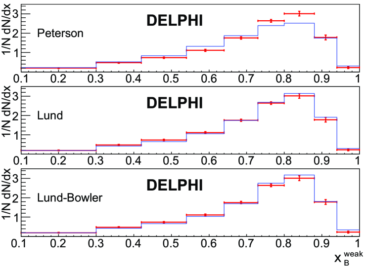
  Figure 7: The result of fitting various hadronisation model functions to the measured $x^{\mathrm{w}eak}_{\mathrm{B}}$ distributions. Points with error bars represent the data, and histograms represent the reweighted Monte-Carlo simulation with the best fit result.

  

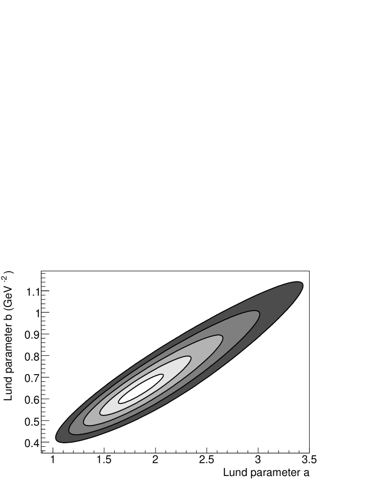
  Figure 8: The one standard deviation (lightest grey) to five standard deviations (darkest grey) contours of the Lund parameters $a$ and $b$. These contours correspond to coverage probabilities of $39.3\%$, $63.2\%$, $77.7\%$, $86.5\%$ and $91.8\%$. The $\chi^{2}$ has been obtained comparing the measured $f(x^{\mathrm{w}eak}_{\mathrm{B}})$ distribution in data to the generated model prediction.

  5 Analytic extraction of the non-perturbative QCD fragmentation function

  The combined DELPHI measurement of $f(x^{\mathrm{w}eak}_{\mathrm{B}})$ is used to extract the b-quark fragmentation function. For this study, the variable $x^{\mathrm{w}eak}_{\mathrm{B}}$ is transformed to $x^{\mathrm{w}eak}_{p}$, which is preferred because it varies exactly between $0$ and $1$. As explained in Section 1, $f(x^{\mathrm{w}eak}_{p})$ as measured in the experiment, can be viewed as the result of perturbative and non-perturbative QCD processes:

  $$f(x^{\mathrm{w}eak}_{p})=\int_{0}^{\infty}{\frac{dx}{x}~{}f_{pert.}(x)~{}f_{non-pert.}\left(\frac{x^{\mathrm{w}eak}_{p}}{x}\right)}~{}.$$ (14)

  In order to separate out the non-perturbative contribution, a choice for the perturbative part must be made. This problem is addressed in two ways:

  • the perturbative contribution is taken from a parton shower Monte-Carlo generator. In this case parameters of the (non-perturbative) fragmentation function $f(x)$ are also fitted within the context of commonly-used hadronisation models;

  • the perturbative contribution is taken to be a NLL QCD calculation and the corresponding non-perturbative component is computed to reproduce the measurements.

  

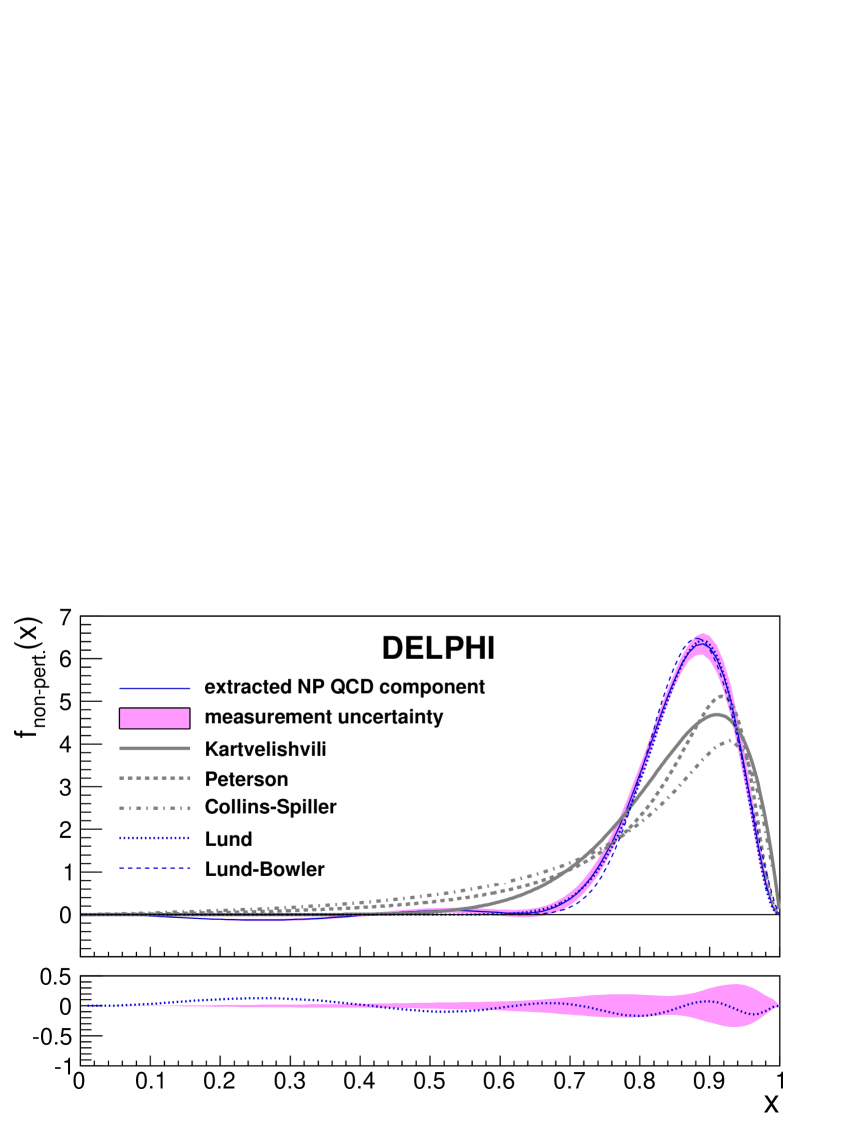
  Figure 9: Dependence of the non-perturbative (NP) QCD component (full line), entering in Equation (14), when the perturbative component is taken from JETSET 7.3. The shaded area corresponds to measurement uncertainties. These uncertainties are correlated for different $x$-values. The other curves correspond to different models whose parameters have been obtained after a fit on present measurements of the fragmentation distribution. The lower plot shows the difference between the extracted non-perturbative QCD component and the fitted Lund model. Note that the variable $x$ used to display the variation of the different distributions is not $x_{p}^{\mathrm{w}eak}$, but the integration variable from Equation (14).

  Model	JETSET 7.3		PYTHIA 6.156
  	Fitted Parameters	$\chi^{2}/NDF$	Fitted Parameters	$\chi^{2}/NDF$
  	and Correlation ($\rho$)		and Correlation ($\rho$)
  Kartvelishvili [35]	$\epsilon_{\mathrm{b}}=10.17\pm 0.37$	$126/6$	$\epsilon_{\mathrm{b}}=13.50\pm 0.56$	57/6
  $x^{\epsilon_{\mathrm{b}}}(1-x)$
  Peterson [18]	$\epsilon_{\mathrm{b}}=(7.4\pm 0.6)\times 10^{-3}$	$83/6$	$\epsilon_{\mathrm{b}}=(4.4\pm 0.4)\times 10^{-3}$	$153/6$
  $\frac{1}{x}\left(1-\frac{1}{x}-\frac{\epsilon_{\mathrm{b}}}{1-x}\right)^{-2}$
  Collins-Spiller[36]	$\epsilon_{\mathrm{b}}=(6.74^{+0.72}_{-0.64})\times 10^{-3}$	$358/6$	$\epsilon_{\mathrm{b}}=(2.56^{+0.38}_{-0.32})\times 10^{-3}$	$322/6$
  $\left(\frac{1-x}{x}+\frac{\epsilon_{\mathrm{b}}(2-x)}{1-x}\right)\left(1+x^{2}\right)\times$
  $\left(1-\frac{1}{x}-\frac{\epsilon_{\mathrm{b}}}{1-x}\right)^{-2}$
  Lund [30]	$a=2.35^{+0.25}_{-0.22}$	$2.3/5$	$a=2.06^{+0.28}_{-0.24}$	$3.8/5$
  $\frac{1}{x}(1-x)^{a}\exp{\left(-\frac{bm_{\mathrm{b}\bot}^{2}}{x}\right)}$	$bm_{\mathrm{b}\bot}^{2}=17.7^{+1.9}_{-1.6}$		$bm_{\mathrm{b}\bot}^{2}=19.8^{+2.4}_{-2.0}$
  	$\left(\rho=89.1\%\right)$		$\left(\rho=89.7\%\right)$
  Lund-Bowler [31]	$a=1.32\pm 0.14$	$12.2/5$	$a=1.02^{+0.15}_{-0.13}$	$5.1/5$
  $\frac{1}{x^{1+bm_{\mathrm{b}\bot}^{2}}}(1-x)^{a}\exp{\left(-\frac{bm_{\mathrm{b}\bot}^{2}}{x}\right)}$	$bm_{\mathrm{b}\bot}^{2}=80.^{+12.}_{-11.}$		$bm_{\mathrm{b}\bot}^{2}=95.^{+13.}_{-12.}$
  	$\left(\rho=75.0\%\right)$		$\left(\rho=76.5\%\right)$

  Table 10: Values of the parameters and of the $\chi^{2}/NDF$ obtained when fitting results from Equation (14), obtained for different models of the non-perturbative QCD component, to the measured b-fragmentation distribution. Results are shown for perturbative QCD components taken from JETSET 7.3 and PYTHIA 6.156. The Lund and Lund-Bowler models have been simplified by assuming that the transverse mass of the b-quark, $m_{\mathrm{b}\bot}$, is a constant.

  The method is based on the use of the Mellin transformation which is appropriate when dealing with integral equations as given in (14). The Mellin transformation of $f(x)$ is:

  $$\tilde{f}(N)=\int_{0}^{\infty}{dx~{}x^{N-1}~{}f(x)}~{},$$ (15)

  where $N$ is a complex variable. For real integer values of $N\geq 2$, the values of $\tilde{f}(N)$ correspond to the moments of the initial $x$ distribution. For physical processes, $x$ is restricted to be within the $[0,1]$ interval. The interest in using Mellin transformed expressions is that Equation (14) becomes a simple product:

  $$\tilde{f}(N)=\tilde{f}_{pert.}(N)\times\tilde{f}_{non-pert.}(N)~{}.$$ (16)

  Having computed distributions of the measured and perturbative QCD components in the $N$-space, the non-perturbative distribution, $\tilde{f}_{non-pert.}(N)$, is obtained from Equation (16). Applying the inverse Mellin transformation on this distribution gives $f_{non-pert.}(x)$ without any need for a model input:

  $$f_{non-pert.}(x)=\frac{1}{2\pi i}\oint{dN~{}\frac{\tilde{f}_{meas.}(N)}{\tilde{f}_{pert.}(N)}~{}x^{-N}}~{},$$ (17)

  in which the integral runs over a contour in the complex $N$-plane. More details on this approach can be found in [33, 32].

  In practice, the Mellin transformed distribution $\tilde{f}_{meas.}(N)$ of the measured distribution has been obtained after having adjusted an analytic expression to the measured distribution in $x^{\mathrm{w}eak}_{p}$, and by applying the Mellin transformation on this fitted function. The following expression, which depends on five parameters, has been used:

  $$f(x)=p_{0}\times\left[p_{1}x^{p_{2}}(1-x)^{p_{3}}+(1-p_{1})x^{p_{4}}(1-x)^{p_{5}}\right]~{},$$ (18)

  where $p_{0}$ is a normalisation coefficient. Values of the parameters have been obtained by comparing, in each bin, the measured bin content with the integral of $f(x)$ over the bin. In order to check the effect of a given choice of parameterisation, the whole procedure has been repeated, replacing the expression of Equation (18) by another function: a cubic spline, with five intervals between $0<x<1$, continuous up to the second derivative, normalised to $1$, and forced to be $0$ at $x=0$ and $x=1$. This function also depends on five parameters. The results obtained with the two parameterisations have been found to be similar [32]. The $N$ representation of the fitted function given in Equation (18) is:

  $$\tilde{f}(N)=p_{0}\left[p_{1}\frac{\Gamma(p_{2}+N)}{\Gamma(p_{2}+p_{3}+N+1)}+(1-p_{1})\frac{\Gamma(p_{4}+N)}{\Gamma(p_{4}+p_{5}+N+1)}\right]~{}.$$ (19)

  The Mellin transformed distribution of the perturbative QCD component in a parton shower Monte-Carlo generator has been obtained from the b-quark $x^{\mathrm{w}eak}_{p}$ distribution generated after gluon radiation. The NLL QCD perturbative component has been computed, directly as a function of $N$, in [34].

  The $x$ distribution of the non-perturbative QCD component extracted in the present approach is independent of any hadronic modelling, but it depends on the procedures adopted to compute the perturbative QCD component.

  5.1 Results obtained using a generated perturbative QCD component

  The JETSET 7.3 and PYTHIA 6.156 event generators, with values of the parameters tuned on DELPHI data at the ${\rm Z}$ pole, have been both used for this study. Events have been produced using the parton shower option of the generator. The corresponding non-perturbative QCD component has been extracted, and is displayed in Figure 9 for the case of JETSET 7.3. The experimental uncertainty on the extracted non-perturbative QCD component is shown as a band. To estimate this uncertainty, a large number of sets of the parameters $p_{1,..,5}$ has been generated, according to their measured error matrix. This matrix has been obtained by propagating the uncertainties of the measured distribution to the fitted parameters. The extraction has been performed for each set of parameters. The root mean square of the resulting distributions for a given value of $x$ has been taken as the uncertainty.

  Parameters of several commonly used hadronisation models have been fitted. In this case, the same perturbative component (as extracted from JETSET 7.3 or PYTHIA 6.156) is used whereas the non-perturbative components are taken from models. These two components are folded according to Equation (14). The integrals of the resulting folding product in each bin are compared to the measurements, and values of the model parameters are fitted. They are given in Table 10 for both event generators, for which the fitted parameters differ, in some cases significantly (illustrating that the non-perturbative component of the fragmentation distribution depends on the algorithm employed to generate the perturbative component). The corresponding distributions, obtained for the different models from the fits with JETSET 7.3, are compared in Figure 9 with the distribution extracted directly from data, using the same perturbative QCD input from JETSET. Figure 10 shows the fragmentation distributions that have been compared in the fit: the measured $x^{\mathrm{w}eak}_{p}$ data points and the folding products resulting from fitted hadronisation models.

  

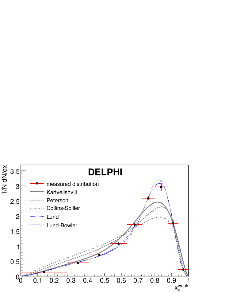
  Figure 10: The measured $x^{\mathrm{w}eak}_{p}$ distribution (data points), compared to the folding products of fitted hadronisation models with the perturbative QCD component from JETSET 7.3 (curves). The fits have been performed by comparing the integral of the resulting folding product in each bin to the measured fragmentation distribution bin content.

  Data favour the Lund and Lund-Bowler models whereas other parameterisations are excluded.

  It has to be noted that values obtained in this approach for model parameters, are compatible with those listed in Table 9, when the same generator is used. The conversion between the Lund and Lund-Bowler $bm_{\mathrm{b}\bot}^{2}$ parameters, as fitted here, and the $b$ fitted in Section 4.4 is done using $m_{\mathrm{b}\bot}^{2}=30.1\ {\rm GeV}^{2}$, which corresponds to the mean value of $m_{\mathrm{b}\bot}^{2}$ in the generated events. The approximation of a constant $m_{\mathrm{b}\bot}^{2}$ is possible due to the small dispersion of this variable in generated events.

  5.2 Results using a perturbative QCD component obtained by an analytic computation based on QCD

  

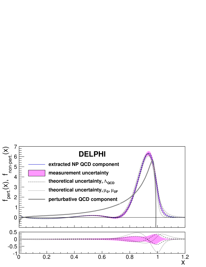
  Figure 11: The $x$-dependence of the non-perturbative QCD component of the measured b-fragmentation distribution (thin full line). This curve is obtained by interpolating corresponding values determined at numerous x values. The shaded area corresponds to measurement uncertainties. These uncertainties are correlated for different $x$-values. The perturbative QCD component (thick full line) is given by the analytic computation of [34]. It has to be complemented by a $\delta$-function containing 5$\%$ of the events, located at $x=1$. The thin lines on both sides of the non-perturbative distribution correspond to $\mu_{0}=\mu_{0F}=\{m_{b}/2,2m_{b}\}$ (dotted lines) and $\Lambda^{(5)}_{{\rm QCD}}=(0.226\pm 0.025)~{}\rm{GeV}$ (dashed lines). Variations induced by the other parameters, $\mu=\mu_{F}=\{Q/2,2Q\}$ and $m_{b}=(4.75\pm 0.25)~{}\rm{GeV}/c^{2}$ are smaller. The lower plot shows the variation of the different uncertainties. Note that the variable $x$ used to display the variation of the different distributions is not $x_{p}^{\mathrm{w}eak}$, but the integration variable from Equation (14).

  

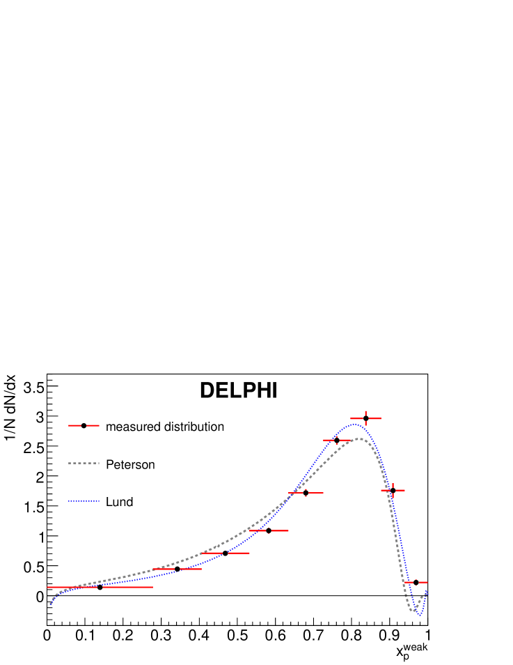
  Figure 12: Fit of the $x^{\mathrm{w}eak}_{p}$-dependence of the fragmentation distribution using an analytic evaluation of the perturbative component from theory, and a model for the non-perturbative component. The histogram with error bars gives the measured $x_{P}$ distribution. The curves correspond to the folding products of the Lund and Peterson hadronisation models with the perturbative QCD component. The fitted parameters for the Lund model are $a=0.551$ and $b=10.27~{}\rm{GeV}^{-2}$. For the Peterson model, $\epsilon_{\mathrm{b}}=0.0038$ has been obtained. The negative parts of the folding products are due to the unphysical region of the perturbative component.

  The perturbative QCD fragmentation function is evaluated according to the approach presented in [34]. Computations are done directly in the $N$-space and are expected to be reliable when $|N|$ is not too large (typically less than 20). This function has singularities at large values of $Re(N)$; in particular, a zero is present at $Re(N)=N_{0}\simeq 41.7$ (this number depends on the exact values assumed for the other parameters entering into the computation). To obtain distributions for the variable $x$ from results in moment space the inverse Mellin transformation is applied, that consists in integrating over a contour in $N$ (see Equation (17)). The choice of the contour has to take into account the presence of singularities at large $Re(N)$. When $x$ gets close to 1, large values of $|N|$ contribute and thus the perturbative fragmentation distribution is not reliable in these regions. This behaviour affects also values of the distribution at lower $x$, which can be understood by the fact that moments of the total distribution are fixed. Unlike the perturbative QCD component which is defined in [34] within the $[0,1]$ interval, the non-perturbative component has to be extended in the region $x>1$. This “non-physical” behaviour comes from the zero of $\tilde{f}_{pert.}(N)$ for $N=N_{0}$ which gives a pole in the expression to be integrated in Equation (17). In other words, this behaviour is directly related to the break-down of the theory for large values of $|N|$ (i.e. for $x$ close to $1$). Using properties of integrals in the complex plane, it can be shown that, for $x>1$, the non-perturbative QCD distribution can be well approximated by $x^{-N_{0}}$. Uncertainties attached to the determination of the theoretical perturbative QCD component are related to the definition of the scales entering into the computation [33, 34].

  The extracted non-perturbative component is given in Figure 11. Its shape depends on the same quantities as those used to evaluate the perturbative distribution, and thus similar variations appear, as drawn also in the Figure. The measurement uncertainty band has been obtained using the same procedure as explained in Section 5.1.

  It has to be noted that the data description in terms of a product of two QCD components, perturbative and non-perturbative, is not directly affected by uncertainties attached to the determination of the perturbative component. This is because the non-perturbative component, as determined in the present approach, compensates for a given choice of method or of parameter values.

  This study indicates that a perturbative QCD component obtained analytically from theory must not be folded with a non-perturbative QCD component taken from a model. All model distributions are physical and cannot compensate for unphysical behaviour of the perturbative computation. This is illustrated in Figure 12, where the measured distribution is shown together with the folding product of the NLL QCD perturbative component and hadronisation models. Model parameters have been obtained from fits to data using the folding product of Equation (14), in the same way as in Section 5.1. The negative parts of the folding products are due to the unphysical behaviour of the perturbative component.

  6 Combined fit of results from all experiments

  In addition to the DELPHI results presented in this paper, the b-quark fragmentation distribution has been measured by ALEPH, OPAL and SLD [27, 28, 29]. These measurements are displayed in Figure 13. Each experiment used a different technique. These four results have been fitted to give a world average b-quark fragmentation distribution and to determine the corresponding non-perturbative QCD component. Global fits of the Lund and Lund-Bowler parameterisations have been also obtained.

  

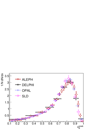
  Figure 13: Comparison between the various measurements of the b-quark fragmentation distribution versus $x^{\mathrm{w}eak}_{\mathrm{B}}$.

  6.1 Combined fit to fragmentation distributions

  Each of the four measurements of the b-quark fragmentation distribution is given with a different choice of binning and has a different number of effective degrees of freedom. In order to obtain a combined distribution, a global fit has been done, using the smooth parameterisation of Equation (18). The $\chi^{2}$ minimised in the fit is the sum of $\chi^{2}$ for the different experiments, computed by comparing, in each bin, the integral of the parameterisation to the measured bin content. The number of degrees of freedom for ALEPH, DELPHI and OPAL are $7$, $7$ and $5$, respectively. When one more degree of freedom is used for one of the three experiments, fits show a large increase in the $\chi^{2}$ value. For SLD, the diagonal error matrix of the $22$ bin values has been used, as the full error matrix was not detailed in [29]. A comparison of the sources of systematic uncertainties between the different analyses shows that, due to the various methods which have been used [27, 28, 29], their origins are very different. As a result, systematic uncertainties from the different experiments have been supposed to be uncorrelated. The fit has been done using both the $x^{\mathrm{w}eak}_{\mathrm{B}}$ and $x^{\mathrm{w}eak}_{p}$ distributions. For $36$ degrees of freedom, the fit of $x^{\mathrm{w}eak}_{\mathrm{B}}$ yields a $\chi^{2}$ of $55.8$ (probability of $2\%$), and the one for $x^{\mathrm{w}eak}_{p}$ yields a $\chi^{2}$ of $67.7$ (probability of $0.1\%$). The large $\chi^{2}$ values are not likely to originate from the smooth function itself, as this function gives a good fit quality to all the individual distributions. The minimum $\chi^{2}$ probability obtained in these fits is $31\%$. This marginal compatibility comes rather from the dispersion of the results mainly between ALEPH and SLD measurements which are respectively peaked on the high and low sides of the distribution. Quoted uncertainties for $x^{\mathrm{w}eak}_{\mathrm{B}}$ and $x^{\mathrm{w}eak}_{p}$ in the following are therefore rescaled by factors $1.24$ and $1.37$, respectively.

  	$x^{\mathrm{w}eak}_{\mathrm{B}}$	$x^{\mathrm{w}eak}_{p}$
  $p_{1}$	$12.97^{+0.77}_{-0.71}$	$12.50^{+0.82}_{-0.76}$
  $p_{2}$	$2.67^{+0.15}_{-0.14}$	$2.63^{+0.17}_{-0.15}$
  $p_{3}$	$2.29^{+0.19}_{-0.17}$	$2.05^{+0.19}_{-0.18}$
  $p_{4}$	$1.45^{+0.28}_{-0.22}$	$1.31^{+0.24}_{-0.20}$
  $p_{5}$	$0.663^{+0.035}_{-0.036}$	$0.664\pm 0.036$

  Table 11: Parameters for the combined world average fragmentation distribution. The quoted uncertainties have been rescaled by factors $1.24$ and $1.37$ for $x^{\mathrm{w}eak}_{\mathrm{B}}$ and $x^{\mathrm{w}eak}_{p}$, respectively, as explained in the text.

  parameter	$p_{1}$	$p_{2}$	$p_{3}$	$p_{4}$	$p_{5}$
  $p_{1}$	$0.546693$
  $p_{2}$	$0.102357$	$0.021477$
  $p_{3}$	$0.008932$	$-0.002099$	$0.032990$
  $p_{4}$	$-0.088755$	$-0.018877$	$0.031327$	$0.059791$
  $p_{5}$	$0.020556$	$0.003772$	$-0.001624$	$-0.007269$	$0.001277$

  Table 12: Error matrix on the fitted parameters of the combined world average fragmentation distribution for the variable $x^{\mathrm{w}eak}_{\mathrm{B}}$. Quoted uncertainties are obtained after applying the scaling factor of $1.24$, as explained in the text.

  parameter	$p_{1}$	$p_{2}$	$p_{3}$	$p_{4}$	$p_{5}$
  $p_{1}$	$0.624398$
  $p_{2}$	$0.118819$	$0.025406$
  $p_{3}$	$0.035693$	$0.002269$	$0.032581$
  $p_{4}$	$-0.070514$	$-0.016499$	$0.024564$	$0.047581$
  $p_{5}$	$0.022370$	$0.004205$	$-0.000181$	$-0.006008$	$0.001316$

  Table 13: The error matrix on the fitted parameters of the combined world average fragmentation distribution for the variable $x^{\mathrm{w}eak}_{p}$. Quoted uncertainties are obtained after applying the scaling factor of $1.37$, as explained in the text.

  The fitted parameters $p_{1},..,p_{5}$ of Equation 18, that represent the world average fragmentation distribution for $x^{\mathrm{w}eak}_{\mathrm{B}}$ and $x^{\mathrm{w}eak}_{p}$ are given in Table 11. The full error matrices on $p_{1},..,p_{5}$ for the two distributions are given in Tables 12 and 13.

  The moments of the combined $x^{\mathrm{w}eak}_{\mathrm{B}}$ distribution are given in Table 14. They have been calculated using the analytic expression of Equation (19) with the fitted values of the parameters $p_{1},..,p_{5}$. The uncertainties have been propagated from the error matrix on the parameters.

  N	moment	uncertainty		N	moment	uncertainty
  				21	$0.0333$	$0.0011$
  2	$0.7092$	$0.0025$		22	$0.0301$	$0.0010$
  3	$0.5334$	$0.0031$		23	$0.0272$	$0.0009$
  4	$0.4158$	$0.0032$		24	$0.0247$	$0.0009$
  5	$0.3322$	$0.0031$		25	$0.0225$	$0.0008$
  6	$0.2703$	$0.0029$		26	$0.0205$	$0.0008$
  7	$0.2231$	$0.0027$		27	$0.0188$	$0.0008$
  8	$0.1864$	$0.0026$		28	$0.0172$	$0.0007$
  9	$0.1573$	$0.0024$		29	$0.0158$	$0.0007$
  10	$0.1339$	$0.0022$		30	$0.0146$	$0.0006$
  11	$0.1148$	$0.0021$		31	$0.0134$	$0.0006$
  12	$0.0992$	$0.0019$		32	$0.0124$	$0.0006$
  13	$0.0862$	$0.0018$		33	$0.0115$	$0.0006$
  14	$0.0754$	$0.0017$		34	$0.0107$	$0.0005$
  15	$0.0662$	$0.0016$		35	$0.0099$	$0.0005$
  16	$0.0585$	$0.0015$		36	$0.0092$	$0.0005$
  17	$0.0518$	$0.0014$		37	$0.0086$	$0.0005$
  18	$0.0462$	$0.0013$		38	$0.0080$	$0.0004$
  19	$0.0413$	$0.0012$		39	$0.0075$	$0.0004$
  20	$0.0370$	$0.0011$		40	$0.0070$	$0.0004$

  Table 14: Moments of the world average fragmentation distribution for $x^{\mathrm{w}eak}_{\mathrm{B}}$. $N=2$ corresponds to the mean value of the distribution. The moments have been calculated using the analytic expression of Equation (19). Uncertainties have been propagated using the error matrix of Table 12.

  The $x^{\mathrm{w}eak}_{\mathrm{B}}$ distribution vanishes in the interval $x^{\mathrm{w}eak}_{\mathrm{B}}\in[0.,~{}0.116=2m_{B}/\sqrt{s}\>]$ whereas the parameterisation of Equation (18) has non zero values in this interval. Nevertheless, the effect of this caveat has been found to be negligible. The integral of the fitted parameterisation in the region $[0.,~{}0.116]$ is $0.0019$. The contribution of this region to the average value of the distribution is of ${\cal O}(10^{-4})$, which is $\sim\!20$ times smaller than the uncertainty. The effect decreases rapidly for higher order moments (${\cal O}(10^{-12})$ for the $10^{th}$ moment).

  6.2 Combined fit of the Lund and Lund-Bowler models

  

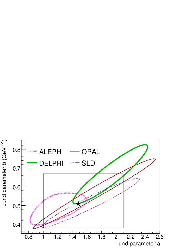
  (a)

  

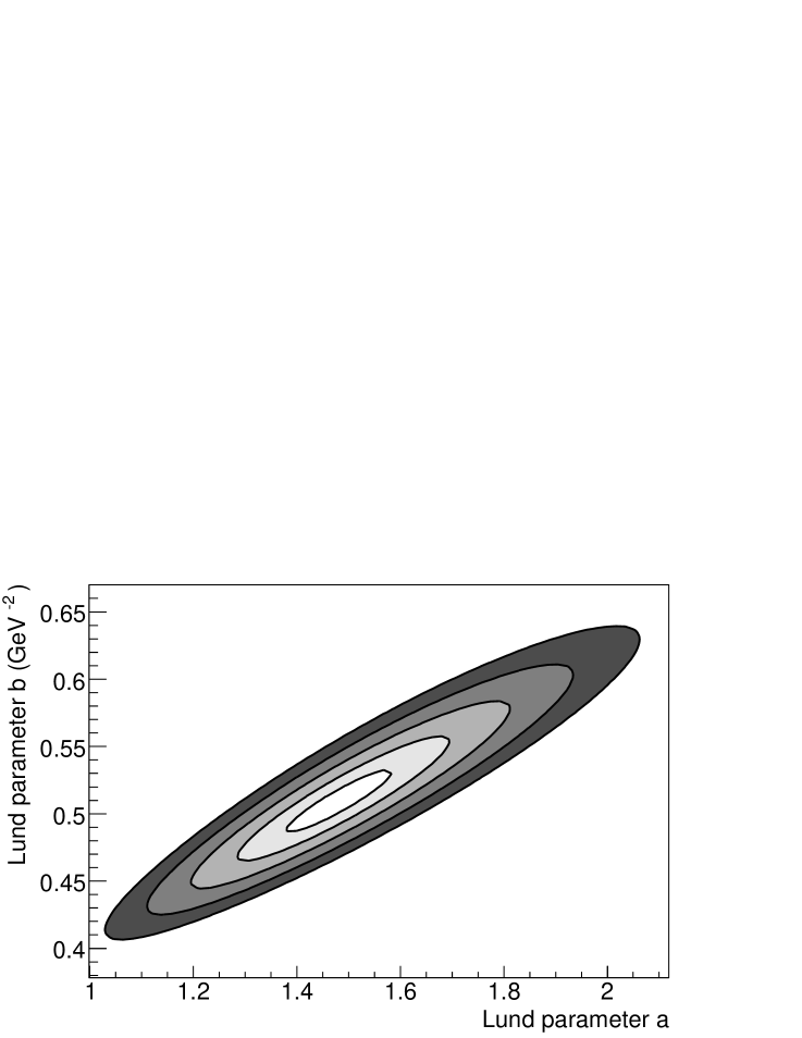
  (b)

  Figure 14: a Contours of $68.3\%$ coverage probability for the $a$ and $b$ Lund parameters corresponding to a separate fit to each experiment and the result obtained in the combined fit marked by $\star$. b Contours varying from $1$ standard deviation (lightest grey) to $5$ standard deviations (darkest grey) for the $a$ and $b$ Lund parameters obtained in the combined fit. These contours correspond to coverage probabilities of $39.3\%$, $63.2\%$, $77.7\%$, $86.5\%$ and $91.8\%$. The box drawn in a corresponds to the area presented in b.

  The $a$ and $b$ parameters of the Lund and Lund-Bowler fragmentation distributions, in the framework of PYTHIA 6.156, have been fitted using the weighting approach described in Section 4.4 and minimising the sum of $\chi^{2}$ for the four experiments. For the Lund-Bowler model, the predicted value $r_{Q}=1$ [31] has been used. The fit yields the Lund parameters $a=1.48^{+0.11}_{-0.10}$; $b=0.509^{+0.024}_{-0.023}\ \rm{GeV}^{-2}$ with a statistical correlation of $\rho=92.6\%$. For the Lund-Bowler parameters the result is $a=0.795^{+0.062}_{-0.059}$; $b=2.28^{+0.13}_{-0.12}\ \rm{GeV}^{-2}$ with a statistical correlation of $\rho=84.2\%$. The minimum $\chi^{2}$ is $39.5$ with $39$ degrees of freedom (probability of $44.6\%$) for the Lund model and $92.4$ for the Lund-Bowler model. Experimental data clearly favours the Lund model to the Lund-Bowler (with $r_{Q}=1$) one.

  Figure 14 shows the $68.3\%$ coverage probability contours for the Lund parameters $a$ and $b$ , as obtained individually for each experiment, compared to the combined fit result. The one to five standard deviations contours of the fitted parameters are also presented.

  Using the parametric form fitted on all measured $x_{p}^{\mathrm{w}eak}$ distributions, given in Table 11, and the direct folding approach described in Section 5.1, the fitted values of the parameters for the Lund fragmentation distribution are: $a=1.48\pm 0.10$; $bm_{{\mathrm{b}}\perp}^{2}=16.62\pm 0.71$ with a statistical correlation of $\rho=90.7\%$. These values are very similar to those given at the beginning of this section, which were obtained by reweighting the simulation event-by-event.

  6.3 Extraction of the non-perturbative QCD component from the combined distribution

  The non-perturbative QCD component has been extracted from the combined fragmentation function obtained in Section 6.1 and from the b-quark fragmentation functions measured separately by each experiment at $e^{+}e^{-}$ colliders [27, 28, 29], including the result from the present analysis. The extraction has been performed using the $x^{\mathrm{w}eak}_{p}$ distributions, following the prescription given in Sections 5.1 and 5.2 using the two perturbative QCD approaches considered in this paper: parton shower Monte-Carlo (both JETSET 7.3 and PYTHIA 6.156) and the theoretical NLL QCD computation from [34]. Comparisons of the results obtained for the combined distribution and for the different experiments are shown in Figure 15. The extracted distributions corresponding to JETSET 7.3 and PYTHIA 6.156 parton shower Monte-Carlo are compared in Figure 16, and show significant differences. The former is clearly softer than the latter. Finally, the extracted distribution corresponding to PYTHIA 6.156 is compared in Figure 17 with the Lund and Lund-Bowler models, obtained in Section 6.2 from the combined fit. There is a good agreement between the Lund model and the extracted non-perturbative QCD component in the peak region. However, from the above figures, together with Figure 9 it is quite apparent that, in spite of some dispersion, all measurements favour a model similar to the Lund or Lund-Bowler shapes. All other parameterisations are excluded.

  

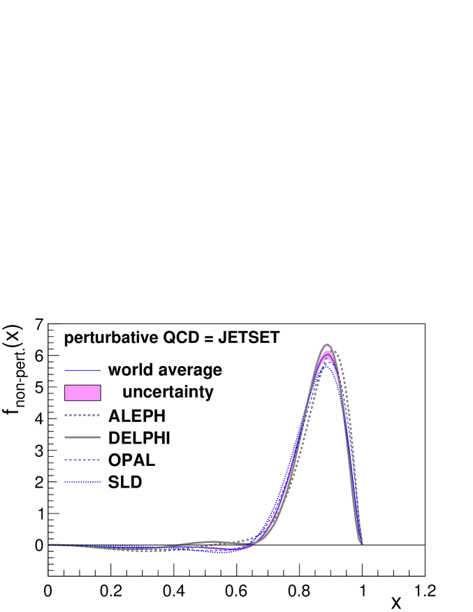
  (a)

  

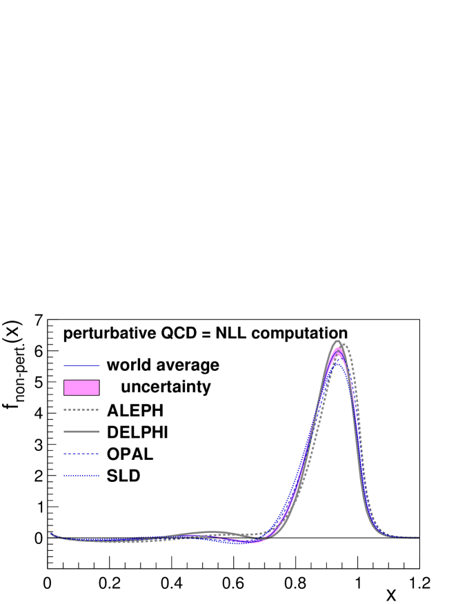
  (b)

  Figure 15: Comparison of the extracted non-perturbative QCD component of the b-quark fragmentation function for the result from the present analysis, ALEPH [27], OPAL [28], SLD [29] and the combined $x^{\mathrm{w}eak}_{p}$ distribution. a The perturbative QCD component has been taken from JETSET 7.3. b The perturbative QCD component has been taken from NLL QCD [34]. The shaded error bands represent the experimental uncertainty of the combined distributions.

  

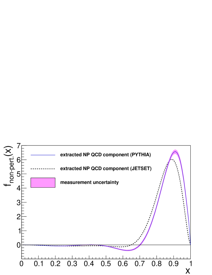
  Figure 16: Comparison of the extracted non-perturbative QCD components from the combined $x^{\mathrm{w}eak}_{p}$ distribution, corresponding to the perturbative QCD components from JETSET 7.3 and PYTHIA 6.156 parton shower Monte-Carlo. The latter is given with its corresponding error band.

  

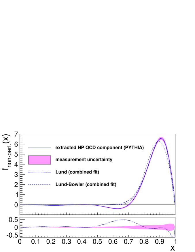
  Figure 17: The extracted non-perturbative QCD component corresponding to PYTHIA 6.156 parton shower Monte-Carlo (presented with error band), compared with the Lund and Lund-Bowler models, obtained from the combined fit. The Lund model is scaled by $1.068$, which corresponds to the integral of the extracted function in the region $x\in[0.701,1.0]$, where it has positive values. For this comparison, $m_{b\bot}^{2}$ has been taken as $30.1\ {\rm GeV}^{2}$, which corresponds to its average value in generated events used for the fit. The lower plot shows the difference between the extracted non-perturbative QCD component corresponding to the PYTHIA 6.156 parton shower Monte-Carlo and the fitted Lund model.

  7 Conclusion

  The fragmentation distribution of the b-quark has been measured using two analyses based on very different approaches. The average fractions of the beam energy taken by weakly decaying b-hadrons are:

  $$\langle x^{\mathrm{w}eak}_{\mathrm{B}}\rangle=0.7140\pm 0.0007{\rm(stat.)}\pm 0.0060{\rm(syst.)}$$ (20)

  and

  $$\langle x^{\mathrm{w}eak}_{\mathrm{B}}\rangle=0.6978\pm 0.0010{\rm(stat.)}\pm 0.0064{\rm(syst.)}~{},$$ (21)

  in the regularised unfolding and weighted fitting analyses, respectively.

  The combined $x^{\mathrm{w}eak}_{\mathrm{B}}$ distribution has been obtained by a fit using the full error matrix of the two analyses. The average value of this distribution is equal to:

  $$\langle x^{\mathrm{w}eak}_{\mathrm{B}}\rangle=0.699\pm 0.011~{}.$$ (22)

  The non-perturbative QCD b-quark fragmentation distribution is obtained from the combined DELPHI measurement in a way that does not depend on any non-perturbative hadronisation model. In order to describe the measured fragmentation function, the non-perturbative distribution has to be folded with the adequate perturbative component, which can be given by a generator, as provided for example by the JETSET/PYTHIA parton shower or by an analytic perturbative QCD computation. It has been demonstrated that for the latter, it is not legitimate to use a physical distribution, as given by commonly used hadronisation models, for the non-perturbative QCD component. Parameters obtained for the non-perturbative component depend on the choice for the perturbative evaluation. This has been illustrated by comparing results obtained with JETSET 7.3, PYTHIA 6.156 and analytic QCD computation.

  The distributions obtained by folding analytically the perturbative and the non-perturbative QCD components are found to be similar to the ones obtained by a Monte-Carlo generator. We stress that the non-perturbative component depends on the exact procedure used to obtain the perturbative one.

  The combined measurement from DELPHI has been compared with expectations from different non-perturbative hadronisation models of the b-quark fragmentation distribution within a Monte Carlo simulation. Only the Lund and Lund-Bowler models give reasonable descriptions of the data, the Lund ansatz being favoured. The parameters of the Lund fragmentation that fit best the data are obtained within the framework of PYTHIA 6.156 to be:

  $$a=1.84^{+0.23}_{-0.21}~{}{\rm and}~{}b=0.642^{+0.073}_{-0.063}\ \rm{GeV}^{-2}$$ (23)

  with a correlation factor $\rho=92.2\%$.

  The present measurement is combined with previous results from the ALEPH, OPAL and SLD experiments and a world averaged b-quark fragmentation distribution is obtained giving:

  $$\langle x^{\mathrm{w}eak}_{\mathrm{B}}\rangle=0.7092\pm 0.0025.$$ (24)

  The corresponding non-perturbative QCD component is also determined. Particularly, a global fit to all the available fragmentation distributions is performed to obtain the parameters of the Lund fragmentation model.

  $$a=1.48^{+0.11}_{-0.10}~{}{\rm and}~{}b=0.509^{+0.024}_{-0.023}\ \rm{GeV}^{-2}$$ (25)

  with a correlation factor $\rho=92.6\%$.

  Acknowledgements

  We are greatly indebted to our technical collaborators, to the members of the CERN-SL Division for the excellent performance of the LEP collider, and to the funding agencies for their support in building and operating the DELPHI detector.
  We acknowledge in particular the support of
  Austrian Federal Ministry of Education, Science and Culture, GZ 616.364/2-III/2a/98,
  FNRS–FWO, Flanders Institute to encourage scientific and technological research in the industry (IWT) and Belgian Federal Office for Scientific, Technical and Cultural affairs (OSTC), Belgium,
  FINEP, CNPq, CAPES, FUJB and FAPERJ, Brazil,
  Ministry of Education of the Czech Republic, project LC527,
  Academy of Sciences of the Czech Republic, project AV0Z10100502,
  Commission of the European Communities (DG XII),
  Direction des Sciences de la Mati$\grave{\mbox{\rm e}}$re, CEA, France,
  Bundesministerium f$\ddot{\mbox{\rm u}}$r Bildung, Wissenschaft, Forschung und Technologie, Germany,
  General Secretariat for Research and Technology, Greece,
  National Science Foundation (NWO) and Foundation for Research on Matter (FOM), The Netherlands,
  Norwegian Research Council,
  State Committee for Scientific Research, Poland, SPUB-M/CERN/PO3/DZ296/2000, SPUB-M/CERN/PO3/DZ297/2000, 2P03B 104 19 and 2P03B 69 23(2002-2004),
  FCT - Fundação para a Ciência e Tecnologia, Portugal,
  Vedecka grantova agentura MS SR, Slovakia, Nr. 95/5195/134,
  Ministry of Science and Technology of the Republic of Slovenia,
  CICYT, Spain, AEN99-0950 and AEN99-0761,
  The Swedish Research Council,
  The Science and Technology Facilities Council, UK,
  Department of Energy, USA, DE-FG02-01ER41155,
  EEC RTN contract HPRN-CT-00292-2002.
  

  Appendix A: Input variables of the $E_{B}^{\rm{weak}}$ reconstruction neural network

  Below is a listing of the main input variables to the neural network used to reconstruct $E_{B}^{\rm{weak}}$ in the regularized unfolding analysis. This variable is an output of the DELPHI inclusive b-physics package BSAURUS and further details of the general approach and specifics of the reconstructed quantities used can be found in [37]. Central to this approach are: (a) the accurate reconstruction of a secondary vertex in each hemisphere as a candidate b-hadron decay vertex and (b) the reconstruction of the quantity: TrackNet. The TrackNet is itself a neural network variable providing, for each charged particle in an event hemisphere, a number ranging between zero and one, related to the probability that the particle originates from the decay of a b-hadron.

  • Rapidities of the particles with the highest, and next highest, values in the event hemisphere.

  • In $2$-jet events, the weakly decaying b-hadron energy as estimated by a TrackNet-weighted sum of charged particle energies in the event hemisphere added to a rapidity-weighted sum for neutral particles. For events with more than $2$ jets, the energy as reconstructed by the rapidity algorithm is taken, which sums over all particles in a hemisphere that pass a selection cut of $y>1.6$. This value provides an efficient separation of particles likely to have originated in b-hadron decays, from those produced in the fragmentation process. Note that jets were reconstructed using the LUCLUS algorithm based on a transverse momentum cutoff parameter value of $d_{\rm join}={\rm PARU}(44)=5.0$ GeV/$c$.

  • Mass of the weakly decaying b-hadron based on all particles with $y>1.6$.

  • Energy of the jet with the highest $b-$tag value calculated by applying the standard DELPHI b-tagging procedure [14] to the jet.

  • The summed charged and neutral energy reconstructed in the event hemisphere and in the event as a whole.

  • An estimate of the missing $p_{T}$ between the b-hadron candidate direction and the thrust axis, calculated using only fragmentation particles (identified by demanding ${\rm TrackNet}<0.5$) in the same hemisphere as the b-hadron candidate and all particles in the opposite hemisphere.

  • The mass of the reconstructed secondary vertex.

  • The polar angle of the b-hadron candidate momentum vector.

  • The thrust value of the event.

  • The total number of all charged and neutral particles.

  • The number of particles passing a TrackNet cut of $>0.5$.

  • For the best electron or muon candidate in the hemisphere, with the correct charge correlation, a number related to the probability that it originates from the b-hadron candidate. Assuming that the track comes from the primary vertex, this number is the probability of getting an impact parameter significance at least as large as that observed.

  • The gap in rapidity between the particle of highest rapidity in the hemisphere (with TrackNet value less than 0.5) and the particle of lowest rapidity (with TrackNet value greater than 0.5).

  Note that some variables used as inputs are not directly correlated with the b-hadron energy but instead provided the network with information about how reliable the other input variables might be, e.g. measures of the total hemisphere energy and the number of particles in the hemisphere that fail selection cuts. The network was thus able to learn during the training phase, e.g. to give extra weight to the variables of event hemispheres when there is a good chance of a hemisphere containing a well reconstructed b-hadron.

  The TrackNet distribution for different track species is shown in Figure 18. Tracks from the b-decay chain are identified with high purity and efficiency via a cut at $\rm{TrackNet}>0.5$.

  

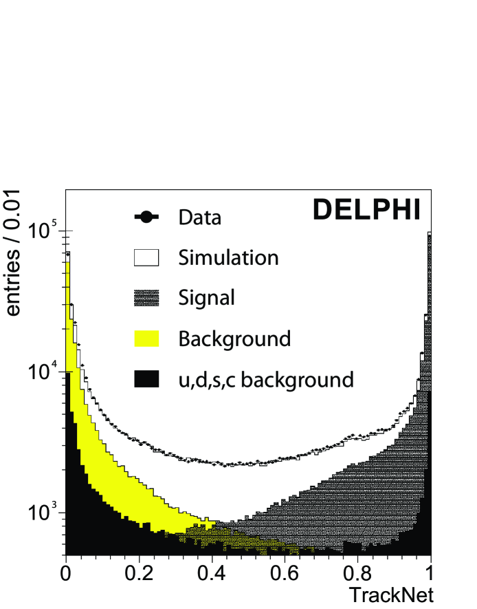
  Figure 18: The TrackNet distribution for different track species. ‘Signal’ refers to tracks originating from the B-hadron decay chain, ‘Background’ are tracks from fragmentation or excited b-hadron decay and ‘u,d,s,c background’ are any tracks in non-b decays of the ${\rm Z}$.

  Appendix B: Regularised unfolding analysis: central values and covariance matrices

  The full bin-to-bin results of the $x^{\mathrm{w}eak}_{\mathrm{B}}$ distribution from the regularised unfolding analysis are listed in Table 15. In each bin the quoted value corresponds to the average of the fitted distribution over this bin:

  $$\frac{\Delta f}{\Delta x^{\mathrm{w}eak}_{\mathrm{B}}}=\frac{1}{x_{\mathrm{B}}^{\mathrm{w}eak,~{}max}-x_{\mathrm{B}}^{\mathrm{w}eak,~{}min}}\int_{x_{\mathrm{B}}^{\mathrm{w}eak,~{}min}}^{x_{\mathrm{B}}^{\mathrm{w}eak,~{}max}}{\frac{df}{dx^{\mathrm{w}eak}_{\mathrm{B}}}~{}dx^{\mathrm{w}eak}_{\mathrm{B}}}~{}.$$

  Values $x_{\mathrm{B}}^{\mathrm{w}eak,~{}max}$ and $x_{\mathrm{B}}^{\mathrm{w}eak,~{}min}$ are the bin limits. The corresponding statistical and total covariance matrices are given in Tables 16 and 17, respectively.

  bin borders	value	stat. error	syst. error	$\sqrt{\sigma_{stat}^{2}+\sigma_{syst}^{2}}$
  0.100 – 0.299	0.154	0.005	0.044	0.044
  0.299 – 0.419	0.458	0.007	0.035	0.036
  0.419 – 0.535	0.724	0.008	0.039	0.039
  0.535 – 0.637	1.041	0.010	0.056	0.057
  0.637 – 0.726	1.635	0.012	0.063	0.064
  0.726 – 0.803	2.632	0.014	0.073	0.075
  0.803 – 0.877	3.091	0.016	0.140	0.141
  0.877 – 0.939	2.033	0.013	0.159	0.159
  0.939 – 1.000	0.300	0.009	0.067	0.067

  Table 15: The unfolding result, per bin, for $f(x^{\mathrm{w}eak}_{\mathrm{B}})$.

  bin	1	2	3	4	5	6	7	8	9
  1	0.021
  2	0.022	0.047
  3	-0.019	0.005	0.069
  4	-0.018	-0.038	0.026	0.103
  5	0.011	-0.011	-0.055	0.026	0.151
  6	0.008	0.019	-0.025	-0.073	0.057	0.194
  7	-0.006	0.003	0.029	-0.022	-0.099	0.057	0.245
  8	-0.001	-0.006	0.003	0.024	-0.018	-0.079	0.025	0.163
  9	0.002	0.001	-0.008	-0.001	0.031	-0.011	-0.085	0.052	0.088

  Table 16: The statistical covariance matrix, in units of $10^{-3}$, for the unfolded bins in $f(x^{\mathrm{w}eak}_{\mathrm{B}})$.

  bin	1	2	3	4	5	6	7	8	9
  1	1.927
  2	0.201	1.296
  3	0.127	0.814	1.552
  4	0.252	0.819	1.252	3.271
  5	0.247	0.717	0.996	2.587	4.120
  6	-0.191	0.167	0.308	1.200	2.222	5.578
  7	-0.928	-1.163	-1.682	-2.615	-2.980	-1.146	19.847
  8	-1.676	-2.818	-3.920	-6.877	-8.562	-4.806	8.827	25.342
  9	-0.669	-1.120	-1.557	-2.725	-3.197	-1.535	3.025	9.007	4.538

  Table 17: The total (i.e. including statistical and systematic uncertainties) covariance matrix, in units of $10^{-3}$, for the unfolded bins in $f(x^{\mathrm{w}eak}_{\mathrm{B}})$.

  Appendix C: Weighted fitting analysis: central values and covariance matrices

  The full bin-to-bin results of the $x^{\mathrm{w}eak}_{\mathrm{B}}$ distribution from the weighted fitting analysis are listed in Table 18. For explanation of the quoted bin values see Appendix A. The corresponding statistical and total covariance matrices are given in Tables 19 and 20, respectively.

  bin borders	value	stat. error	syst. error	$\sqrt{\sigma_{stat}^{2}+\sigma_{syst}^{2}}$
  0.100 – 0.299	0.180	0.003	0.010	0.010
  0.299 – 0.419	0.445	0.008	0.028	0.029
  0.419 – 0.535	0.746	0.012	0.034	0.036
  0.535 – 0.637	1.220	0.017	0.060	0.062
  0.637 – 0.726	1.947	0.025	0.082	0.086
  0.726 – 0.803	2.694	0.040	0.062	0.074
  0.803 – 0.877	2.790	0.040	0.133	0.139
  0.877 – 0.939	1.600	0.043	0.137	0.144
  0.939 – 1.000	0.268	0.020	0.086	0.088

  Table 18: The unfolding result, per bin, for $f(x^{\mathrm{w}eak}_{\mathrm{B}})$.

  bin	1	2	3	4	5	6	7	8	9
  1	0.007
  2	0.021	0.058
  3	0.026	0.077	0.138
  4	0.021	0.063	0.166	0.292
  5	-0.003	-0.015	0.024	0.210	0.613
  6	-0.015	-0.061	-0.140	-0.124	0.526	1.587
  7	0.024	0.055	0.017	-0.098	-0.172	0.415	1.603
  8	0.033	0.082	0.158	0.216	-0.040	-0.707	-0.183	1.838
  9	-0.002	-0.005	-0.008	0.001	0.079	0.190	-0.067	-0.352	0.416

  Table 19: The statistical covariance matrix, in units of $10^{-3}$, for the unfolded bins in $f(x^{\mathrm{w}eak}_{\mathrm{B}})$.

  bin	1	2	3	4	5	6	7	8	9
  1	0.106
  2	0.292	0.841
  3	0.248	0.818	1.323
  4	-0.025	0.202	1.602	3.849
  5	-0.397	-0.806	0.855	4.463	7.415
  6	-0.337	-1.027	-1.057	-0.042	2.877	5.440
  7	-0.048	-0.656	-3.257	-7.428	-9.097	-0.679	19.353
  8	-0.432	-1.745	-3.326	-5.212	-6.299	-1.804	13.991	20.555
  9	0.286	0.902	0.677	-0.202	-0.564	-0.573	-2.817	-6.084	7.864

  Table 20: The total (i.e. including statistical and systematic uncertainties) covariance matrix, in units of $10^{-3}$, for the unfolded bins in $f(x^{\mathrm{w}eak}_{\mathrm{B}})$.

  Appendix D: Combined DELPHI result: covariance matrices

  The statistical and total covariance matrices for the combined DELPHI result in bins of the $f(x^{\mathrm{w}eak}_{\mathrm{B}})$ distribution are given in Tables 21 and 22, respectively.

  bin	1	2	3	4	5	6	7	8	9
  1	0.019
  2	0.034	0.069
  3	0.022	0.049	0.072
  4	0.025	0.050	0.086	0.181
  5	0.044	0.078	0.061	0.194	0.422
  6	0.076	0.133	0.098	0.177	0.468	0.819
  7	0.077	0.144	0.137	0.181	0.257	0.629	0.833
  8	0.078	0.146	0.137	0.243	0.337	0.449	0.568	0.755
  9	0.037	0.063	0.054	0.110	0.207	0.240	0.140	0.308	0.227

  Table 21: The statistical covariance matrix, in units of $10^{-3}$, for the unfolded bins in $f(x^{\mathrm{w}eak}_{\mathrm{B}})$. Elements are scaled by a factor 1.71.

  bin	1	2	3	4	5	6	7	8	9
  1	0.408
  2	-0.139	1.013
  3	0.554	0.346	1.403
  4	-0.134	0.730	1.013	2.514
  5	-0.109	0.073	0.723	2.393	3.729
  6	-0.122	0.044	-0.216	0.398	2.056	4.850
  7	-0.111	-0.319	-1.721	-3.815	-4.596	-0.505	14.838
  8	-0.372	-1.123	-2.413	-3.922	-4.605	-2.410	10.305	14.939
  9	0.075	-0.210	-0.441	-1.102	-1.149	0.123	1.550	3.507	2.373

  Table 22: The total (i.e. including statistical and systematic uncertainties) covariance matrix, in units of $10^{-3}$, for the unfolded bins in $f(x^{\mathrm{w}eak}_{\mathrm{B}})$. Elements are scaled by a factor 1.71.

  A study of the
  b-quark fragmentation function
  with the DELPHI detector at LEP I
  and an averaged distribution
  obtained at the ${\rm Z}$ Pole