Cohomology classes represented by measured foliations, and Mahler’s question for interval exchanges

Abstract.

A translation surface on $(S,\Sigma)$ gives rise to two transverse measured foliations ${\mathcal{F}},{\mathcal{G}}$ on $S$ with singularities in $\Sigma$, and by integration, to a pair of cohomology classes $[{\mathcal{F}}],\,[{\mathcal{G}}]\in H^{1}(S,\Sigma;{\mathbb{R}})$. Given a measured foliation ${\mathcal{F}}$, we characterize the set of cohomology classes $\mathbf{b}$ for which there is a measured foliation ${\mathcal{G}}$ as above with $\mathbf{b}=[{\mathcal{G}}]$. This extends previous results of Thurston [Th] and Sullivan [Su].

We apply this to two problems: unique ergodicity of interval exchanges and flows on the moduli space of translation surfaces. For a fixed permutation $\sigma\in\mathcal{S}_{d}$, the space ${\mathbb{R}}^{d}_{+}$ parametrizes the interval exchanges on $d$ intervals with permutation $\sigma$. We describe lines $\ell$ in ${\mathbb{R}}^{d}_{+}$ such that almost every point in $\ell$ is uniquely ergodic. We also show that for $\sigma(i)=d+1-i$, for almost every $s>0$, the interval exchange transformation corresponding to $\sigma$ and $(s,s^{2},\ldots,s^{d})$ is uniquely ergodic. As another application we show that when $k=|\Sigma|\geq 2,$ the operation of ‘moving the singularities horizontally’ is globally well-defined. We prove that there is a well-defined action of the group $B\ltimes{\mathbb{R}}^{k-1}$ on the set of translation surfaces of type $(S,\Sigma)$ without horizontal saddle connections. Here $B\subset\operatorname{SL}(2,{\mathbb{R}})$ is the subgroup of upper triangular matrices.

1. Introduction

1.1. Motivating questions and nonsensical pictures

To introduce the problems discussed in this paper, consider some pictures. Suppose that ${\bf{a}}=(a_{1},\ldots,a_{d})$ is a vector with positive entries, $I=\left[0,\sum a_{i}\right)$ is an interval, $\sigma$ is a permutation on $d$ symbols, and $\mathcal{T}=\mathcal{T}_{\sigma}({\bf{a}}):I\to I$ is the interval exchange obtained by cutting up $I$ into segments of lengths $a_{i}$ and permuting them according to $\sigma$. A fruitful technique for studying the dynamical properties of $\mathcal{T}$ is to consider it as the return map to a transverse segment along the vertical foliation in a translation surface, i.e. a union of polygons with edges glued pairwise by translations. See Figure 1.1 for an example with one polygon; note that the interval exchange determines the horizontal coordinates of vertices, but there are many possible choices of the vertical coordinates.

Figure 1.1. Masur’s construction: an interval exchange embedded in a one-polygon translation surface.

Given a translation surface $q$ with a transversal, one may deform it by applying the horocycle flow, i.e. deforming the polygon with the linear map

$${h_{s}=\left(\begin{matrix}1&s\\ 0&1\end{matrix}\right).}$$ (1)

The return map to a transversal in $h_{s}q$ depends on $s$, so we get a one-parameter family $\mathcal{T}_{s}$ of interval exchange transformations (Figure 1.2). For sufficiently small $s$, one has $\mathcal{T}_{s}=\mathcal{T}_{\sigma}({\bf{a}}(s)),$ where ${\bf{a}}(s)={\bf{a}}+s\mathbf{b}$ is a line segment, whose derivative $\mathbf{b}=(b_{1},\ldots,b_{d})$ is determined by the heights of the vertices of the polygon. We will consider an inverse problem: given a line segment ${\bf{a}}(s)={\bf{a}}+s\mathbf{b}$, does there exist a translation surface $q$ such that for all sufficiently small $s$, $\mathcal{T}_{\sigma}({\bf{a}}(s))$ is the return map along vertical leaves to a transverse segment in $h_{s}q$? Attempting to interpret this question with pictures, we see that some choices of $\mathbf{b}$ lead to a translation surface while others lead to nonsensical pictures – see Figure 1.3. The solution to this problem is given by Theorem 5.3.

Figure 1.2. The horocycle action gives a linear one parameter family of interval exchanges

Figure 1.3. The choice $\mathbf{b}=(2,1,-1,-2)$ (left) gives a translation surface but what about $\mathbf{b}=(0,3,-1,-2)$?

Now consider a translation surface $q$ with two singularities. We may consider the operation of moving one singularity horizontally with respect to the other. That is, at time $s$, the line segments joining one singularity to the other are made longer by $s$, while line segments joining a singularity to itself are unchanged. For small values of $s$, one obtains a new translation surface $q_{s}$ by examining the picture. But for large values of $s$, some of the segments in the figure cross each other and it is not clear whether the operation defined above gives rise to a well-defined surface. Our Theorem 11.2 shows that the operation of moving the zeroes is well-defined for all values of $s$, provided one rules out the obvious obstruction that two singularities connected by a horizontal segment collide.

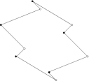
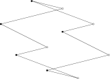
Figure 1.4. The singularity $\circ$ is moved to the right with respect to $\bullet$, and the picture becomes nonsensical.

1.2. Main geometrical result

Let $S$ be a compact oriented surface of genus $g\geq 2$ and $\Sigma\subset S$ a finite subset. A translation surface structure on $(S,\Sigma)$ is an atlas of charts into the plane, whose domains cover $S\smallsetminus\Sigma$, and such that the transition maps are translations. Such structures arise naturally in complex analysis and in the study of interval exchange transformations and polygonal billiards and have been the subject of intensive research, see the recent surveys [MT, Zo].

Several geometric structures on the plane can be pulled back to $S\smallsetminus\Sigma$ via the atlas, among them the foliations of the plane by horizontal and vertical lines. We call the resulting oriented foliations of $S\smallsetminus\Sigma$ the horizontal and vertical foliation respectively. Each can be completed to a singular foliation on $S$, with a pronged singularity at each point of $\Sigma$. Label the points of $\Sigma$ by $\xi_{1},\ldots,\xi_{k}$ and fix natural numbers $r_{1},\ldots,r_{k}$. We say that the translation surface is of type $\mathbf{r}=(r_{1},\ldots,r_{k})$ if the horizontal and vertical foliations have a $2(r_{j}+1)$-pronged singularity at each $\xi_{j}$.

By pulling back $dy$ (resp. $dx$) from the plane, the horizontal (vertical) foliation arising from a translation surface structure is equipped with a transverse measure, i.e. a family of measures on each arc transverse to the foliation which is invariant under holonomy along leaves. We will call an oriented singular foliation on $S$, with singularities in $\Sigma$, which is equipped with a transverse measure a measured foliation on $(S,\Sigma)$. We caution the reader that we deviate from the convention adopted in several papers on this subject, by considering the number and orders of singularities as part of the structure of a measured foliation; we call these the type of the foliation. In other words, we do not consider two measured foliations which differ by a Whitehead move to be the same.

Integrating the transverse measures gives rise to two well-defined cohomology classes in the relative cohomology group $H^{1}(S,\Sigma;{\mathbb{R}})$. That is we obtain a map

$$\mathrm{hol}:\left\{\mathrm{translation\ surfaces\ on\ }(S,\Sigma)\right\}\to\left(H^{1}(S,\Sigma;{\mathbb{R}})\right)^{2}.$$

This map is a local homeomorphism and serves to give coordinate charts to the set of translation surfaces (see §2.1 for more details), but it is not globally injective. For example, precomposing with a homeomorphism which acts trivially on homology may change a marked translation surface structure but does not change its image in under hol; see [Mc] for more examples. On the other hand it is not hard to see that the pair of horizontal and vertical measured foliations associated to a translation surface uniquely determine it, and hence the question arises of reconstructing the translation surface from just the cohomological data recorded by hol. Our main theorems give results in this direction.

To state them we define the set of (relative) cycles carried by ${\mathcal{F}}$, denoted $H_{+}^{\mathcal{F}}$, to be the image in $H_{1}(S,\Sigma;{\mathbb{R}})$ of all (possibly atomic) transverse measures on ${\mathcal{F}}$ (see §2.5).

Theorem 1.1.

Suppose ${\mathcal{F}}$ is a measured foliation on $(S,\Sigma)$, and $\mathbf{b}\in H^{1}(S,\Sigma;{\mathbb{R}})$. Then the following are equivalent:

1. There is a measured foliation ${\mathcal{G}}$ on $(S,\Sigma)$, everywhere transverse to ${\mathcal{F}}$ and of the same type, such that ${\mathcal{G}}$ represents $\mathbf{b}$.

2. Possibly after replacing $\mathbf{b}$ with $-\mathbf{b}$, for any $\delta\in H_{+}^{{\mathcal{F}}}$, $\mathbf{b}\cdot\delta>0$.

After proving Theorem 1.1 we learned from F. Bonahon that it has a long and interesting history. Similar result were proved by Thurston [Th] in the context of train tracks and measured laminations, and by Sullivan [Su] in a very general context involving foliations. Bonahon neglected to mention his own contribution [Bon]. Our result is a ‘relative version’ in that we control the type of the foliation, and need to be careful with the singularities. This explains why our definition of $H_{+}^{\mathcal{F}}$ includes the relative cycles carried by critical leaves of ${\mathcal{F}}$. The proof we present here is close to the one given by Thurston.

The arguments proving Theorem 1.1 imply the following stronger statement (see §2 for detailed definitions):

Theorem 1.2.

Given a topological singular foliation ${\mathcal{F}}$ on $(S,\Sigma)$, let $\widetilde{\mathcal{H}}({\mathcal{F}})$ denote the set of marked translation surfaces whose vertical foliation is topologically equivalent to ${\mathcal{F}}$. Let $\mathbb{A}({\mathcal{F}})\subset H^{1}(S,\Sigma;{\mathbb{R}})$ denote the set of cohomology classes corresponding to (non-atomic) transverse measures on ${\mathcal{F}}$. Let $\mathbb{B}({\mathcal{F}})\subset H^{1}(S,\Sigma;{\mathbb{R}})$ denote the set of cohomology classes that pair positively with all elements of $H^{\mathcal{F}}_{+}\subset H_{1}(S,\Sigma)$. Then

$$\mathrm{hol}:\widetilde{\mathcal{H}}({\mathcal{F}})\to\mathbb{A}({\mathcal{F}})\times\mathbb{B}({\mathcal{F}})$$

is a homeomorphism.

1.3. Applications

We present two applications of Theorem 1.1. The first concerns the generic properties of interval exchange transformations. Let $\sigma$ be a permutation on $d$ symbols and let ${\mathbb{R}}^{d}_{+}$ be the vectors ${\bf{a}}=(a_{1},\ldots,a_{d})$ for which $a_{i}>0,\,i=1,\ldots,d.$ The pair ${\bf{a}},\sigma$ determines an interval exchange $\mathcal{T}_{\sigma}({\bf{a}})$ by subdividing the interval $I_{\bf{a}}=\left[0,\sum a_{i}\right)$ into $d$ subintervals of lengths $a_{i}$, which are permuted according to $\sigma$. In 1982 Masur [Mas1] and Veech [Ve2] confirmed a conjecture of Keane, proving (assuming that $\sigma$ is irreducible) that almost every ${\bf{a}}$, with respect to Lebesgue measure on ${\mathbb{R}}^{d}_{+}$, is uniquely ergodic, i.e. the only invariant measure for $\mathcal{T}_{\sigma}({\bf{a}})$ is Lebesgue measure. On the other hand Masur and Smillie [MS] showed that the set of non-uniquely ergodic interval exchanges is large in the sense of Hausdorff dimension. A basic problem is to understand the finer structure of the set of non-uniquely ergodic interval exchanges. Specifically, motivated by analogous developments in diophantine approximations, we will ask: For which curves $\ell\subset{\mathbb{R}}^{d}_{+}$ is the non-uniquely ergodic set of zero measure, with respect to the natural measure on the curve? Which properties of a measure $\mu$ on ${\mathbb{R}}^{d}_{+}$ guarantee that $\mu$-a.e. ${\bf{a}}$ is uniquely ergodic?

In this paper we obtain several results in this direction, involving three ingredients: a curve in ${\mathbb{R}}^{d}_{+}$; a measure supported on the curve; and a dynamical property of interval exchanges. The goal will be to understand the dynamical properties of points in the support of the measure. We state these results, and some open questions in this direction, in §6. To illustrate them we state a special case, which may be thought of as an interval exchanges analogue of a famous result of Sprindzhuk (Mahler’s conjecture, see e.g. [Kl, §4]):

Theorem 1.3.

For $d\geq 2,$ let

$${{\bf{a}}(x)=\left(x,x^{2},\ldots,x^{d}\right)}$$ (2)

and let $\sigma(i)=d+1-i$. Then ${\bf{a}}(x)$ is uniquely ergodic for Lebesgue a.e. $x>0$.

Identifying two translation structures which differ by a precomposition with an orientation preserving homeomorphism of $S$ which fixes each point of $\Sigma$ we obtain the stratum ${\mathcal{H}}(\mathbf{r})$ of translation surfaces of type $\mathbf{r}$. There is an action of $G=\operatorname{SL}(2,{\mathbb{R}})$ on ${\mathcal{H}}(\mathbf{r})$, and its restriction to the subgroup $\{h_{s}\}$ as in (1) is called the horocycle flow. To prove our results on unique ergodicity we employ the strategy, introduced in [KeMasSm], of lifting interval exchanges to translation surfaces, and studying the dynamics of the $G$-action on ${\mathcal{H}}(\mathbf{r})$. Specifically we use quantitative nondivergence estimates [MiWe] for the horocycle flow. Theorem 1.1 is used to characterize the lines in ${\mathbb{R}}^{d}_{+}$ which may be lifted to horocycle paths.

The second application concerns an operation of ‘moving singularities with respect to each other’ which has been discussed in the literature under various names (cf. [Zo, §9.6]) and which we now define. Let $\widetilde{\mathcal{H}}(\mathbf{r})$ be the stratum of marked translation surfaces of type $\mathbf{r}$, i.e. two translation surface structures are equivalent if they differ by precomposition by a homeomorphism of $S$ which fixes $\Sigma$ and is isotopic to the identity rel $\Sigma$. Integrating transverse measures as above induces a well-defined map $\widetilde{\mathcal{H}}(\mathbf{r})\to H^{1}(S,\Sigma;{\mathbb{R}}^{2})$ which can be used to endow $\widetilde{\mathcal{H}}(\mathbf{r})$ (resp. ${\mathcal{H}}(\mathbf{r})$) with the structure of an affine manifold (resp. orbifold), such that the natural map $\widetilde{\mathcal{H}}(\mathbf{r})\to{\mathcal{H}}(\mathbf{r})$ is an orbifold cover. We describe foliations on $\widetilde{\mathcal{H}}(\mathbf{r})$ which descend to well-defined foliations on ${\mathcal{H}}(\mathbf{r})$. The two summands in the splitting

$${H^{1}(S,\Sigma;{\mathbb{R}}^{2})\cong H^{1}(S,\Sigma;{\mathbb{R}})\oplus H^{1}(S,\Sigma;{\mathbb{R}})}$$ (3)

induce two foliations on $\widetilde{\mathcal{H}}(\mathbf{r})$, which we call the real foliation and imaginary foliation respectively. Also, considering the exact sequence in cohomology

$${H^{0}(S;{\mathbb{R}}^{2})\to H^{0}(\Sigma;{\mathbb{R}}^{2})\to H^{1}(S,\Sigma;{\mathbb{R}}^{2})\stackrel{{\scriptstyle\mathrm{Res}}}{{\to}}H^{1}(S;{\mathbb{R}}^{2})\to\{0\},}$$ (4)

we obtain a natural subspace $\ker\mathrm{Res}\subset H^{1}(S,\Sigma;{\mathbb{R}}^{2})$, consisting of the cohomology classes which vanish on the subspace of ‘absolute periods’ $H_{1}(S)\subset H_{1}(S,\Sigma).$ The foliation induced on $\widetilde{\mathcal{H}}(\mathbf{r})$ is called the REL foliation or kernel foliation. Finally, intersecting the leaves of the real foliation with those of the REL foliation yields the real REL foliation. It has leaves of dimension $k-1$ (where $k=|\Sigma|$). Two nearby translation surfaces $q$ and $q^{\prime}$ are in the same plaque if the integrals of the flat structures along all closed curves are the same on $q$ and $q^{\prime}$, and if the integrals of curves joining distinct singularities only differ in their horizontal component. Intuitively, $q^{\prime}$ is obtained from $q$ by fixing one singularity as a reference point and moving the other singularities horizontally. Understanding this foliation is important for the study of the dynamics of the horocycle flow. It was studied in some restricted settings in [EsMarMo, CaWo], where it was called Horiz.

The leaves of the kernel foliation, and hence the real REL foliation, are equipped with a natural translation structure, modeled on the vector space $\ker\,\mathrm{Res}\cong H^{0}(\Sigma;{\mathbb{R}})/H^{0}(S,{\mathbb{R}})$. One sees easily that the leaf of $q$ is incomplete if, when moving along the leaf, a saddle connection on $q$ is made to have length zero, i.e. if ‘singularities collide’. Using Theorems 1.1 and 1.2 we show in Theorem 11.2 that this is the only obstruction to completeness of leaves. This implies that on a large set, the leaves of real REL are the orbits of an action. More precisely, let ${\mathcal{Q}}$ be the set of translation surfaces with no horizontal saddle connections, in a finite cover $\hat{{\mathcal{H}}}$ of ${\mathcal{H}}({\mathbf{r}})$ (we take a finite cover to make ${\mathcal{H}}({\mathbf{r}})$ into a manifold). This is a set of full measure which is invariant under the group $B$ of upper triangular matrices in $G$. We show that it coincides with the set of complete real REL leaves. Let $F$ denote the group $B\ltimes{\mathbb{R}}^{k-1}$, where $B$ acts on ${\mathbb{R}}^{k-1}$ via

$$\left(\begin{matrix}a&b\\ 0&1/a\end{matrix}\right)\cdot\vec{v}=a\vec{v}.$$

We prove:

Theorem 1.4.

The group $F$ acts on ${\mathcal{Q}}$ continuously and affinely, preserving the natural measure, and leaving invariant the subset of translation surfaces of area one. The action of $B$ is the same as that obtained by restricting the $G$-action, and the ${\mathbb{R}}^{k-1}$-action is transitive on each real REL leaf in ${\mathcal{Q}}$.

Note that while the $F$-action is continuous, ${\mathcal{Q}}$ is not complete: it is the complement in $\hat{{\mathcal{H}}}$ of a dense countable union of proper affine submanifolds with boundary. Also note that the leaves of the real foliation or the kernel foliation are not orbits of a group action on $\hat{{\mathcal{H}}}$ — but see [EsMarMo] for a related discussion of pseudo-group-actions.

1.4. Organization of the paper

We present the proof of Theorem 1.1 in §3 and of Theorem 1.2, in §4. We interpret these theorems in the language of interval exchanges in §5. This interpretation furnishes a link between line segments in the space of interval exchanges, and horocycle paths in a corresponding stratum of translation surfaces: it turns out that the line segments which may be lifted to horocycle paths form a cone in the tangent space to interval exchange space, and this cone can be explicitly described in terms of a bilinear form studied by Veech. We begin §6 with a brief discussion of Mahler’s question in diophantine approximation, and the question it motivates for interval exchanges. We then state in detail our results for generic properties of interval exchanges. The proofs of these results occupy §7–§10. Nondivergence results for horocycles make it possible to analyze precisely the properties of interval exchanges along a line segment, in the cone of directions described in §12. To obtain information about curves we approximate them by line segments, and this requires the quantitative nondivergence results obtained in [MiWe]. In §11 we prove our results concerning real REL. These sections may be read independently of §6–§10. We conclude with a discussion which connects real REL with some of the objects encountered in §7-§10.

1.5. Acknowledgements

We thank John Smillie for many valuable discussions. We thank Francis Bonahon for pointing out the connection between our Theorem 1.1 and previous work of Sullivan and Thurston. The authors were supported by BSF grant 2004149, ISF grant 584/04 and NSF grant DMS-0504019.

2. Preliminaries

In this section we recall some standard facts and set our notation. For more information we refer the reader to [MT, Zo] and the references therein.

2.1. Strata of translation surfaces

Let $S,\,\Sigma=(\xi_{1},\ldots,\xi_{k}),\,\mathbf{r}=(r_{1},\ldots,r_{k})$ be as in the introduction. A translation structure (resp., a marked translation structure) of type $\mathbf{r}$ on $(S,\Sigma)$ is an equivalence class of $(U_{\alpha},\varphi_{\alpha})$, where:

• $(U_{\alpha},\varphi_{\alpha})$ is an atlas of charts for $S\smallsetminus\Sigma$;

• the transition functions $\varphi_{\beta}\circ\varphi^{-1}_{\alpha}$ are of the form

  $${\mathbb{R}}^{2}\ni\vec{x}\mapsto\vec{x}+c_{\alpha,\beta};$$

• around each $\xi_{j}\in\Sigma$ the charts glue together to form a cone point with cone angle $2\pi(r_{j}+1)$.

By definition $(U_{\alpha},\varphi_{\alpha}),\ (U^{\prime}_{\beta},\varphi^{\prime}_{\beta})$ are equivalent if there is an orientation preserving homeomorphism $h:S\to S$ (for a marked structure, isotopic to the identity via an isotopy fixing $\Sigma$), fixing all points of $\Sigma$, such that $(U_{\alpha},\varphi_{\alpha})$ is compatible with $\left(h(U^{\prime}_{\beta}),\varphi^{\prime}_{\beta}\circ h^{-1}\right).$ Thus the equivalence class ${\mathbf{q}}$ of a marked translation surface is a subset of that of the corresponding translation surface $q$, and we will say that ${\mathbf{q}}$ is obtained from $q$ by specifying a marking, $q$ from ${\mathbf{q}}$ by forgetting the marking, and write $q=\pi({\mathbf{q}})$. Note that our convention is that singularities are labelled.

Pulling back $dx$ and $dy$ from the coordinate charts we obtain two well-defined closed 1-forms, which we can integrate along any path $\alpha$ on $S$. If $\alpha$ is a cycle or has endpoints in $\Sigma$ (a relative cycle), then the result, which we denote by

$${\mathrm{hol}}(\alpha,{\mathbf{q}})=\left(\begin{matrix}x(\alpha,{\mathbf{q}})\\ y(\alpha,{\mathbf{q}})\end{matrix}\right)\in{\mathbb{R}}^{2},$$

depends only on the homology class of $\alpha$ in $H_{1}(S,\Sigma)$. We let ${\mathrm{hol}}({\mathbf{q}})={\mathrm{hol}}(\cdot,{\mathbf{q}})$ be the corresponding element of $H^{1}(S,\Sigma;{\mathbb{R}}^{2})$, with coordinates $x({\mathbf{q}}),y({\mathbf{q}})$ in $H^{1}(S,\Sigma;{\mathbb{R}})$.

A saddle connection for $q$ is a straight segment which connects singularities and does not contain singularities in its interior.

The set of all (marked) translation surfaces on $(S,\Sigma)$ of type $\mathbf{r}$ is called the stratum of (marked) translation surface of type $\mathbf{r}$ and is denoted by ${\mathcal{H}}(\mathbf{r})$ (resp. $\widetilde{\mathcal{H}}(\mathbf{r})$). We have suppressed the dependence on $\Sigma$ from the notation since for a given type $\mathbf{r}$ there is an isomorphism between the corresponding set of translation surfaces on $(S,\Sigma)$ and on $(S,\Sigma^{\prime})$ for any other finite subset $\Sigma^{\prime}=\left(\xi^{\prime}_{1},\ldots,\xi^{\prime}_{k}\right)$.

The map ${\mathrm{hol}}:\widetilde{\mathcal{H}}\to H^{1}(S,\Sigma;{\mathbb{R}}^{2})$ just defined gives local charts for $\widetilde{\mathcal{H}}$, endowing it (resp. ${\mathcal{H}}$) with the structure of an affine manifold (resp. orbifold). To see how this works, fix a triangulation $\tau$ of $S$ with vertices in $\Sigma$. Then ${\mathrm{hol}}({\mathbf{q}})$ associates a vector in the plane to each oriented edge in $\tau$, and hence associates an oriented Euclidean triangle to each oriented triangle of $\tau$. If all the orientations are consistent, then a translation structure with the same holonomy as ${\mathbf{q}}$ can be realized explicitly by gluing the Euclidean triangles to each other. Let $\widetilde{\mathcal{H}}_{\tau}$ be the set of all translation structures obtained in this way (we say that $\tau$ is realized geometrically in such a structure). Then the restriction ${\mathrm{hol}}:\widetilde{\mathcal{H}}_{\tau}\to H^{1}(S,\Sigma;{\mathbb{R}}^{2})$ is injective and maps onto an open subset. Conversely every ${\mathbf{q}}$ admits some geometric triangulation (e.g. a Delaunay triangulation as in [MS]) and hence ${\mathcal{H}}$ is covered by the ${\mathcal{H}}_{\tau}$, and so these provide an atlas for a linear manifold structure on $\widetilde{\mathcal{H}}$. We should remark that a topology on $\widetilde{\mathcal{H}}$ can be defined independently of this, by considering nearly isometric comparison maps between different translation structures, and that this topology is the same as that induced by the charts of hol.

Let $\operatorname{Mod}(S,\Sigma)$ denote the mapping class group, i.e. the orientation preserving homeomorphisms of $S$ fixing $\Sigma$ pointwise, up to an isotopy fixing $\Sigma$. The map hol is $\operatorname{Mod}(S,\Sigma)$-equivariant. This means that for any $\varphi\in\operatorname{Mod}(S,\Sigma)$, ${\mathrm{hol}}({\mathbf{q}}\circ\varphi)=\varphi_{*}{\mathrm{hol}}({\mathbf{q}})$, which is nothing more than the linearity of the holonomy map with respect to its first argument.

One can show that the $\operatorname{Mod}(S,\Sigma)$-action on $\widetilde{\mathcal{H}}$ is properly discontinuous. Thus ${\mathcal{H}}=\widetilde{\mathcal{H}}/\operatorname{Mod}(S,\Sigma)$ is a linear orbifold and $\pi:\widetilde{\mathcal{H}}\to{\mathcal{H}}$ is an orbifold covering map. Since $\operatorname{Mod}(S,\Sigma)$ contains a finite index torsion-free subgroup (see e.g. [Iv, Chap. 1]), there is a finite cover $\hat{{\mathcal{H}}}\to{\mathcal{H}}$ such that $\hat{{\mathcal{H}}}$ is a manifold, and we have

$${\dim{\mathcal{H}}=\dim\widetilde{\mathcal{H}}=\dim\hat{{\mathcal{H}}}=\dim H^{1}(S,\Sigma;{\mathbb{R}}^{2})=2(2g+k-1).}$$ (5)

The Poincaré Hopf index theorem implies that

$${\sum r_{j}=2g-2.}$$ (6)

There is an action of $G=\operatorname{SL}(2,{\mathbb{R}})$ on ${\mathcal{H}}$ and on $\widetilde{\mathcal{H}}$ by post-composition on each chart in an atlas. The projection $\pi:\widetilde{\mathcal{H}}\to{\mathcal{H}}$ is $G$-equivariant. The $G$-action is linear in the homology coordinates, namely, given a marked translation surface structure ${\mathbf{q}}$ and $\gamma\in H_{1}(S,\Sigma)$, and given $g\in G$, we have

$${{\mathrm{hol}}(\gamma,g{\mathbf{q}})=g\cdot{\mathrm{hol}}(\gamma,{\mathbf{q}}),}$$ (7)

where on the right hand side, $g$ acts on ${\mathbb{R}}^{2}$ by matrix multiplication.

We will write

$$g_{t}=\left(\begin{array}[]{cc}e^{t/2}&0\\ 0&e^{-t/2}\end{array}\right),\ \ \ \ \ r_{\theta}=\left(\begin{array}[]{cc}\cos\theta&-\sin\theta\\ \sin\theta&\cos\theta\end{array}\right).$$

2.2. Interval exchange transformations

Suppose $\sigma$ is a permutation on $d$ symbols. For each

$${\bf{a}}\in{\mathbb{R}}^{d}_{+}=\left\{(a_{1},\ldots,a_{d})\in{\mathbb{R}}^{d}:\forall i,\,a_{i}>0\right\}$$

we have an interval exchange transformation $\mathcal{T}_{\sigma}({\bf{a}})$ defined by dividing the interval

$$I=I_{\bf{a}}=\left[0,\sum a_{i}\right)$$

into subintervals of lengths $a_{i}$ and permuting them according to $\sigma.$ It is customary to take these intervals as closed on the left and open on the right, so that the resulting map has $d-1$ discontinuities and is left-continuous.

More precisely, set $x_{0}=x^{\prime}_{0}=0$ and for $i=1,\ldots,d$,

$${x_{i}=x_{i}({\bf{a}})=\sum_{j=1}^{i}a_{j},\ \ \ x^{\prime}_{i}=x^{\prime}_{i}({\bf{a}})=\sum_{j=1}^{i}a_{\sigma^{-1}(j)}=\sum_{\sigma(k)\leq i}a_{k};}$$ (8)

then for every $x\in I_{i}=[x_{i-1},x_{i})$ we have

$${\mathcal{T}(x)=\mathcal{T}_{\sigma}({\bf{a}})(x)=x-x_{i-1}+x^{\prime}_{\sigma(i)-1}=x-x_{i}+x^{\prime}_{\sigma(i)}.}$$ (9)

In particular, if (following Veech [Ve1]) we let $Q$ be the alternating bilinear form given by

$${Q({\mathbf{e}}_{i},{\mathbf{e}}_{j})=\left\{\begin{matrix}1&&i>j,\,\sigma(i)<\sigma(j)\\ -1&&i<j,\,\sigma(i)>\sigma(j)\\ 0&&\mathrm{otherwise}\end{matrix}\right.}$$ (10)

where ${\mathbf{e}}_{1},\ldots,{\mathbf{e}}_{d}$ is the standard basis of ${\mathbb{R}}^{d}$, then

$$\mathcal{T}(x)-x=Q({\bf{a}},{\mathbf{e}}_{i}).$$

An interval exchange $\mathcal{T}:I\to I$ is said to be minimal if there are no proper closed $\mathcal{T}$-invariant subsets of $I$. We say that $\mathcal{T}$ is uniquely ergodic if the only invariant measure for $\mathcal{T}$, up to scaling, is Lebesgue measure. We will say that ${\bf{a}}\in{\mathbb{R}}^{d}_{+}$ is minimal or uniquely ergodic if $\mathcal{T}_{\sigma}({\bf{a}})$ is.

Below we will assume that $\sigma$ is irreducible, i.e. there is no $k<d$ such that $\sigma$ leaves the subset $\{1,\ldots,k\}$ invariant, and admissible (in Veech’s sense), see §2.3. For the questions about interval exchanges which we will study, these hypotheses on $\sigma$ entail no loss of generality.

It will be helpful to consider a more general class of maps which we call generalized interval exchanges. Suppose $J$ is a finite union of intervals. A generalized interval exchange $\mathcal{T}:J\to J$ is an orientation preserving piecewise isometry of $J$, i.e. it is a map obtained by subdividing $J$ into finitely many subintervals and re-arranging them to obtain $J$. These maps are not often considered because studying their dynamics easily reduces to studying interval exchanges. However they will arise naturally in our setup.

2.3. Measured foliations, transversals, and interval exchange induced by a translation surface

Given a surface $S$ and a finite $\Sigma\subset S$, a singular foliation (on $S$ with singularities in $\Sigma$) is a foliation ${\mathcal{F}}$ on $S\smallsetminus\Sigma$ such that for any $z\in\Sigma$ there is $k=k_{z}\geq 3$ such that ${\mathcal{F}}$ extends to form a $k$-pronged singularity at $z$. A singular foliation ${\mathcal{F}}$ is orientable if there is a continuous choice of a direction on each leaf. If ${\mathcal{F}}$ is orientable then $k_{z}$ is even for all $z$. Leaves which meet the singularities are called critical. A transverse measure on a singular foliation ${\mathcal{F}}$ is a family of measures defined on arcs transverse to the foliation and invariant under restriction to subsets and isotopy through transverse arcs. A measured foliation is a singular foliation equipped with a transverse measure, which we further require has no atoms and has full support (no open arc has measure zero). We will only consider orientable singular foliations which can be equipped with a transverse measure. This implies that the surface $S$ is decomposed into finitely many domains on each of which the foliation is either minimal (any ray is dense) or periodic (any leaf is periodic). A periodic component is also known as a cylinder. These components are separated by saddle connections.

Given a flat surface structure ${\mathbf{q}}$ on $S$, pulling back via charts the vertical and horizontal foliations on ${\mathbb{R}}^{2}$ give oriented singular foliations on $S$ called the vertical and horizontal foliations, respectively. Transverse measures are defined by integrating the pullbacks of $dx$ and $dy$, i.e. they correspond to the holonomies $x({\mathbf{q}})$ and $y({\mathbf{q}})$. Conversely, given two oriented everywhere transverse measured foliations on $S$ with singularities in $\Sigma$, one obtains an atlas of charts as in §2.1 by integrating the measured foliation. I.e., for each $z\in S\smallsetminus\Sigma$, a local coordinate system is obtained by taking a simply connected neighborhood $U\subset S\smallsetminus\Sigma$ of $z$ and defining the two coordinates of $\varphi(w)\in{\mathbb{R}}^{2}$ to be the integral of the measured foliations along some path connecting $z$ to $w$ (where the orientation of the foliations is used to determine the sign of the integral). One can verify that this procedure produces an atlas with the required properties.

We will often risk confusion by using the symbol ${\mathcal{F}}$ to denote both a measured foliation and the corresponding singular foliation supporting it. A singular foliation is called minimal if any noncritical leaf is dense, and uniquely ergodic if there is a unique (up to scaling) transverse measure on $S$ which is supported on noncritical leaves. Where confusion is unavoidable we say that $q$ is minimal or uniquely ergodic if its vertical foliation is.

At a singular point $p\in\Sigma$ with $k$ prongs, a small neighborhood of $p$ divides into $k$ foliated disks, glued along leaves of ${\mathcal{F}}$, which we call foliated half-disks. A foliated half-disk is either contained in a single periodic component or in a minimal component.

Now let ${\mathcal{F}}$ be a singular foliation on a surface $S$ with singularities in $\Sigma$. We will consider three kinds of transversals to ${\mathcal{F}}$.

• We define a transverse system to be an injective map $\gamma:J\to S$ where $J$ is a finite union of intervals $J_{i}$, the restriction of $\gamma$ to each interval $J_{i}$ is a smooth embedding, the image of the interior of $\gamma$ intersects every non-critical leaf of ${\mathcal{F}}$ transversally, and does not intersect $\Sigma$.

• We define a judicious curve to be a transverse system $\gamma:J\to S$ with $J$ connected, such that $\gamma$ begins and ends at singularities, and the interior of $\gamma$ intersects all leaves including critical ones.

• We say a transverse system $\gamma$ is special if all its components are of the following types (see Figure 2.1):

  • For every foliated half-disk $D$ of a singularity $p\in\Sigma$ which is contained in a minimal component, there is a component of $\gamma$ whose interior intersects $D$ and terminating at $p$. This component of $\gamma$ meets $\Sigma$ at only one endpoint.

  • For every periodic component (cylinder) $P$ of ${\mathcal{F}}$, $\gamma$ contains one arc crossing $P$ and joining two singularities on opposite sides of $P$.

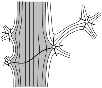
Figure 2.1. A special transverse system cuts across periodic components and into minimal components.

Note that since every non-critical leaf in a minimal component is dense, the non-cylinder edges of a special transverse system can be made as short as we like, without destroying the property that they intersect every non-critical leaf.

In each of these cases, we can parametrize points of $\gamma$ using the transverse measure, and consider the first return map to $\gamma$ when moving up along vertical leaves. When $\gamma$ is a judicious curve, this is an interval exchange transformation which we denote by $\mathcal{T}({\mathcal{F}},\gamma)$, or by $\mathcal{T}(q,\gamma)$ when ${\mathcal{F}}$ is the vertical foliation of $q$. Then there is a unique choice of $\sigma$ and ${\bf{a}}$ with $\mathcal{T}({\mathcal{F}},\gamma)=\mathcal{T}_{\sigma}({\bf{a}})$, and with $\sigma$ an irreducible admissible permutation. The corresponding number of intervals is

$${d=2g+|\Sigma|-1;}$$ (11)

note that $d=\dim H^{1}(S,\Sigma;{\mathbb{R}})=\frac{1}{2}\dim{\mathcal{H}}$ if $q\in{\mathcal{H}}$. The return map to a transverse system is a generalized interval exchange. We denote it also by $\mathcal{T}({\mathcal{F}},\gamma)$. In each of the above cases, any non-critical leaf returns to $\gamma$ infinitely many times.

If $\gamma$ is a transversal to ${\mathcal{F}}$ then $\mathcal{T}({\mathcal{F}},\gamma)$ completely determines the transverse measure on ${\mathcal{F}}.$ In particular the vertical foliation of $q$ is uniquely ergodic (minimal) if and only if $\mathcal{T}(q,\gamma)$ is for some (any) transverse system $\gamma$.

There is an inverse construction which associates with an irreducible permutation $\sigma$ a surface $S$ of genus $g$, and a $k$-tuple ${\mathbf{r}}$ satisfying (6), such that the following holds. For any ${\bf{a}}\in{\mathbb{R}}^{d}_{+}$ there is a translation surface structure $q\in{\mathcal{H}}({\mathbf{r}})$, and a transversal $\gamma$ on $S$ such that $\mathcal{T}_{\sigma}({\bf{a}})=\mathcal{T}(q,\gamma).$ Variants of this construction can be found in [ZeKa, Mas1, Ve2]. Veech’s admissibility condition amounts to requiring that there is no transverse arc on $S$ for which $\mathcal{T}(q,\gamma)$ has fewer discontinuities. Fixing $\sigma$, we say that a flat structure $q$ on $S$ is a lift of ${\bf{a}}$ if there is a judicious curve $\gamma$ on $S$ such that $\mathcal{T}(q,\gamma)=\mathcal{T}_{\sigma}({\bf{a}})$. It is known that for any $\sigma$, there is a stratum ${\mathcal{H}}$ such that all lifts of all ${\bf{a}}$ lie in ${\mathcal{H}}$. We call it the stratum corresponding to $\sigma$.

2.4. Decomposition associated with a transverse system

Suppose ${\mathcal{F}}$ is an oriented singular foliation on $(S,\Sigma)$ and $\gamma:J\to S$ is a transverse system to ${\mathcal{F}}$. There is an associated cellular decomposition $\mathcal{B}=\mathcal{B}(\gamma)$ of $(S,\Sigma)$ defined as follows. Let $\mathcal{T}=\mathcal{T}({\mathcal{F}},\gamma)$ be the generalized interval exchange corresponding to $\gamma$.

The 2-cells in $\mathcal{B}$ correspond to the intervals of continuity of $\mathcal{T}$. For each such interval $I$, the corresponding cell consists of the union of interiors of leaf intervals beginning at $I$ and ending at $\mathcal{T}(I)$. Hence it fibers over $I$ and hence has the structure of an open topological rectangle. The boundary of a 2-cell lies in $\gamma$ and in certain segments of leaves, and the union of these form the 1-skeleton. The 0-skeleton consists of points of $\Sigma$, endpoints of $\gamma$, and points of discontinuity of $\mathcal{T}$ and $\mathcal{T}^{-1}$. Edges of the 1-skeleton lying on $\gamma$ will be called transverse edges and edges lying on ${\mathcal{F}}$ will be called leaf edges. Leaf edges inherit an orientation from ${\mathcal{F}}$ and transverge edges inherit the transverse orientation induced by ${\mathcal{F}}$.

Note that opposite boundaries of a 2-cell could come from the same points in $S$: a particular example occurs for a special transverse system, where if there is a transverse edge crossing a cylinder, that cylinder is obtained as a single 2-cell with its bottom and top edges identified. Such a 2-cell is called a cylinder cell.

It is helpful to consider a spine for $\mathcal{B}$, which we denote $\chi=\chi(\gamma)$, and is composed of the 1-skeleton of $\mathcal{B}$ together with one leaf $\ell_{R}$ for every rectangle $R$, traversing $R$ from bottom to top. The spine is closely related to Thurston’s train tracks; indeed, if we delete from $\chi$ the singular points $\Sigma$ and the leaf edges that meet them, and collapse each element of the transversal $\gamma$ to a point, we obtain a train track that ‘carries ${\mathcal{F}}$’ in Thurston’s sense. But note that keeping the deleted edges allows us to keep track of information relative to $\Sigma$, and in particular, to keep track of the saddle connections in ${\mathcal{F}}$.

2.5. Transverse cocycles, homology and cohomology

We now describe cycles supported on a foliation ${\mathcal{F}}$ and their dual cocycles.

We will see that a transverse measure $\mu$ on ${\mathcal{F}}$ defines an element $[c_{\mu}]\in H_{1}(S,\Sigma)$, expressed concretely as a cycle $c_{\mu}$ in the spine of $\chi(\gamma)$ of a transverse system. Poincaré duality identifies $H_{1}(S,\Sigma)$ with $H^{1}(S\smallsetminus\Sigma)$, and the dual $[d_{\mu}]$ of $[c_{\mu}]$ is represented by the cochain corresponding to integrating the measure $\mu$.

If $\mu$ has no atoms, then in fact we obtain $[c^{\prime}_{\mu}]\in H_{1}(S\smallsetminus\Sigma)$, and its dual $[d^{\prime}_{m}u]$ lies in $H^{1}(S,\Sigma)$. The natural maps $H_{1}(S\smallsetminus\Sigma)\to H_{1}(S,\Sigma)$ and $H^{1}(S,\Sigma)\to H^{1}(S\smallsetminus\Sigma)$ take $[c^{\prime}_{\mu}]$ to $[c_{\mu}]$ and $[d^{\prime}_{\mu}]$ to $[d_{\mu}]$ respectively.

We will now describe these constructions in more detail.

Let $\gamma$ be a transverse system and $\chi(\gamma)$ the spine of its associated complex $\mathcal{B}(\gamma)$ as above. Given $\mu$ we define a 1-chain on $\chi$ as follows. For each rectangle $R$ whose bottom side is an interval $\kappa$ in $\gamma$, set $\mu(R)=\mu({\rm int}\,\kappa)$ (using the interior is important here because of possible atoms in the boundary). For each leaf edge $f$ of $\mathcal{B}$, set $\mu(\{f\})$ to be the transverse measure of $\mu$ across $f$ (which is 0 unless the leaf $f$ is an atom of $\mu$). The 1-chain $x=\sum_{R}\mu(R)\ell_{R}+\sum_{f}\mu(\{f\})f+z$ may not be a cycle, but we note that invariance of $\mu$ implies that, on each component of $\gamma$, teh sum of measures taken with sign (ingoing vs. outgoing) is 0, so that $\partial x$ restricted to each component is null-homologous. Hence by ‘coning off’ $\partial x$ in each component of $\gamma$ we can obtain a cycle of the form:

$${c_{\mu}=\sum_{R\ \mathrm{rectangle}}\mu(R)\ell_{R}+\sum_{f\ \mathrm{leaf\ edge\ of\ }\mathcal{B}}\mu(\{f\})f+z,}$$ (12)

where $z$ is a 1-chain supported in $\gamma$ such that $\partial z=-\partial x$. Invariance and additivity of $\mu$ imply that the homology class in $H_{1}(S,\Sigma)$ is independent of the choice of $\gamma$.

The cochain $d_{\mu}$ is constructed as follows: in any product neighborhood $U$ for ${\mathcal{F}}$ in $S\smallsetminus\Sigma$, integration of $\mu$ gives a map $U\to{\mathbb{R}}$, constant along leaves (but discontinuous at atomic leaves). On any oriented path in $U$ with endpoints off the atoms, the value of the cochain is obtained by mapping endpoints to ${\mathbb{R}}$ and subtracting. Via subdivision this extends to to a cochain defined on 1-chains whose boundary misses atomic leaves. This cochain is a cocycle via additivity and invariance of the measures, and suffices to give a cohomology class (or one may extend it to all 1-chains by a suitable chain-homotopy perturbing vertices on atomic leaves slightly).

In the case with no atoms, we note that the expression for $c_{\mu}$ has no terms of the form $\mu(\{f\})f$, and hence we get a cocycle in $S\smallsetminus\Sigma$. The definition of the cochain extends in that case to neighborhoods of singular points, and evaluates consistently on relative 1-chains, giving a class in $H^{1}(S,\Sigma)$.

A cycle corresponding to a transverse measure will be called a (relative) cycle carried by ${\mathcal{F}}$. The set of all (relative) cycles carried by ${\mathcal{F}}$ is a convex cone in $H_{1}(S,\Sigma;{\mathbb{R}})$ which we denote by $H^{\mathcal{F}}_{+}$. Since we allow atomic measures, we can think of (positively oriented) saddle connections or closed leaves in ${\mathcal{F}}$ as elements of $H^{\mathcal{F}}_{+}$. Another way of constructing cycles carried by ${\mathcal{F}}$ is the Schwartzman asymptotic cycle construction [Sc]. These are projectivized limits of long loops which are mostly in ${\mathcal{F}}$ but may be closed by short segments transverse to ${\mathcal{F}}$. It is easy to see that $H^{{\mathcal{F}}}_{+}\cap H_{1}(S)$ is the convex cone over the asymptotic cycles, or equivalently the image of the non-atomic transverse measures, and that $H^{{\mathcal{F}}}_{+}$ is the convex cone over asymptotic cycles and positive saddle connections in ${\mathcal{F}}$. Generically (when ${\mathcal{F}}$ is uniquely ergodic and contains no saddle connections) ${\mathcal{H}}_{+}^{\mathcal{F}}$ is one-dimensional and is spanned by the so-called asymptotic cycle of ${\mathcal{F}}$.

2.6. Intersection pairing

Via Poincaré duality, the canonical pairing on $H^{1}(S,\Sigma)\times H_{1}(S,\Sigma)$ becomes the intersection pairing on $H_{1}(S\smallsetminus\Sigma)\times H_{1}(S,\Sigma)$. In the former case we denote this pairing by $(d,c)\mapsto d(c)$, and in the latter, by $(c,c^{\prime})\mapsto c\cdot c^{\prime}$. Suppose ${\mathcal{F}}$ and ${\mathcal{G}}$ are two mutually transverse oriented singular foliations, with transverse measures $\mu$ and $\nu$ respectively. If we allow $\mu$ but not $\nu$ to have atoms, then $[c_{\mu}]\in H_{1}(S,\Sigma)$ and $[c_{\nu}]\in H_{1}(S\smallsetminus\Sigma)$ so we have the intersection pairing

$${c_{\nu}\cdot c_{\mu}=d_{\nu}(c_{\mu})=\int_{S}\nu\times\mu.}$$ (13)

In other words we integrate the transverse measure of ${\mathcal{G}}$ along the leaves of ${\mathcal{F}}$, and then integrate against the transverse measure of ${\mathcal{F}}$. (The sign of $\nu\times\mu$ should be chosen so that it is positive when the orientation of ${\mathcal{G}}$ agrees with the transverse orientation of ${\mathcal{F}}$). We can see this explicitly by choosing a transversal $\gamma$ for ${\mathcal{F}}$ lying in the leaves of ${\mathcal{G}}$ . Then the cochain representing $d_{\nu}$ is 0 along $\gamma$, and using the form (12) we have

$${d_{\nu}(c_{\mu})=\sum_{R}\mu(R)\int_{\ell_{R}}\nu\,+\sum_{f}\mu(\{f\})\int_{f}\nu.}$$ (14)

2.6.1. Judicious case

Now suppose $\gamma$ is a judicious transversal. In this case the pairing of $H^{1}(S,\Sigma)$ and $H_{1}(S,\Sigma)$ has a concrete form which we will use in §5.

There is a cell decomposition $\mathcal{D}$ of $S$ that is dual to $\mathcal{B}$, defined as follows. Because $\gamma$ intersects all leaves, and terminates at $\Sigma$ on both ends, each rectangle $R$ of $\mathcal{B}$ has exactly one point of $\Sigma$ on each of its leaf edges. Connect these two points by a transverse arc in $R$ and let $\mathcal{D}^{1}$ be the union of these arcs. $\mathcal{D}^{1}$ cuts $S$ into a disk $\mathcal{D}^{2}$, bisected by $\gamma$. Indeed, upward flow from $\gamma$ encounters $\mathcal{D}^{1}$ in a sequence of edges which is the upper boundary of the disk, and downward flow encounters the lower boundary which goes through the edges of $\mathcal{D}^{1}$ in a permuted order, in fact exactly the permutation $\sigma$ of the interval exchange $\mathcal{T}({\mathcal{F}},\gamma)$.

A class in $H^{1}(S,\Sigma)$ is determined by its values on the (oriented) edges of $\mathcal{D}^{1}$, and in fact this gives a basis, which we can label by the intervals of continuity of $\mathcal{T}({\mathcal{F}},\gamma)$ (the condition that the sum is 0 around the boundary of the disk is satisfied automatically). The Poincaré dual basis for $H_{1}(S\smallsetminus\Sigma)$ is given by the loops $\hat{\ell}_{R}$ obtained by joining the endpoints of $\ell_{R}$ along $\gamma$.

The pairing restricted to non-negative homology is computed by the form $Q$ of (10). Ordering the rectangles $R_{1},\ldots,R_{d}$ according to their bottom arcs along $\gamma$ and writing $\hat{\ell}_{i}=\hat{\ell}_{R_{i}}$, we note that $\hat{\ell}_{i}$ and $\hat{\ell}_{j}$ have nonzero intersection number precisely when the order of $i$ and $j$ is reversed by $\sigma$ (i.e. $(i-j)(\sigma(i)-\sigma(j))<0$), and in particular (accounting for sign),

$${\hat{\ell}_{i}\cdot\hat{\ell}_{j}=Q({\mathbf{e}}_{i},{\mathbf{e}}_{j}).}$$ (15)

In other words, $Q$ is the intersection pairing on $H_{1}(S\smallsetminus\Sigma)\times H_{1}(S\smallsetminus\Sigma)$ with the given basis (note that this form is degenerate, as the map $H_{1}(S\smallsetminus\Sigma)\to H_{1}(S,\Sigma)$ has a kernel).

3. The lifting problem

In this section we prove Theorem 1.1.

Proof of Theorem 1.1.

We first explain the easy direction (1) $\Longrightarrow$ (2). Since ${\mathcal{F}}$ is everywhere transverse to ${\mathcal{G}}$, and the surface is connected, reversing the orientation of ${\mathcal{G}}$ if necessary we can assume that positively oriented paths in leaves of ${\mathcal{F}}$ always cross ${\mathcal{G}}$ from left to right. Therefore, using (13) and (14), we find that $\mathbf{b}(\delta)>0$ for any $\delta\in{\mathcal{H}}_{+}^{\mathcal{F}}$.

Before proving the converse we indicate the idea of proof. We will consider a sequence of finer and finer cell decompositions associated to a shrinking sequence of special transverse systems. As the transversals shrink, the associated train tracks split, each one being carried by the previous one. We examine the weight that a representative of $\mathbf{b}$ places on the vertical leaves in the cells of these decompositions (roughly speaking the branches of the associated train tracks). If any of these remain non-positive for all time, then a limiting argument produces an invariant measure on ${\mathcal{F}}$ which has non-positive pairing with $\mathbf{b}$, a contradiction. Hence eventually all cells have positive ‘heights’ with respect to $\mathbf{b}$, and can be geometrically realized as rectangles. The proof is made complicated by the need to keep track of the singularities, and in particular by the appearance of cylinder cells in the decomposition.

Fix a special transverse system $\gamma$ for ${\mathcal{F}}$ (see §2.3), and let $\mathcal{B}=\mathcal{B}(\gamma)$ be the corresponding cell decomposition as in §2.4. Given a path $\alpha$ on $S$ which is contained in a leaf of ${\mathcal{F}}$ and begins and ends in transverse edges of $\mathcal{B}$, we will say that $\alpha$ is parallel to saddle connections if there is a continuous family of arcs $\alpha_{s}$ contained in leaves, where $\alpha_{0}=\alpha$, $\alpha_{1}$ is a union of saddle connections in ${\mathcal{F}}$, and the endpoints of each $\alpha_{s}$ are in $\gamma$.

We claim that for any $N$ there is a special transverse system $\gamma_{N}\subset\gamma$ such that the following holds: for any leaf edge $e$ of $\mathcal{B}_{N}=\mathcal{B}(\gamma_{N})$, either $e$ is parallel to saddle connections or, when moving along $e$ from bottom to top, we return to $\gamma\smallsetminus\gamma_{N}$ at least $N$ times before returning to $\gamma_{N}$. Indeed, if the claim is false then for some $N$ and any special $\gamma^{\prime}\subset\gamma$ there is a leaf edge $e^{\prime}$ in $\mathcal{B}_{N}$ which is not parallel to saddle connections, and starts and ends at points $x$, $y$ in $\gamma^{\prime}$, making at most $N$ crossings with $\gamma\smallsetminus\gamma^{\prime}$. Now take $\gamma^{\prime}_{j}$ to be shorter and shorter special transverse subsystems of $\gamma$, denote the corresponding edge by $e_{j}$ and the points by $x_{j},\,y_{j}$. Passing to a subsequence, we find that $x_{j},y_{j}$ converge to points in $\Sigma$ and $e_{j}$ converges to a concatentation of at most $N$ saddle connections joining these points. In particular, for large enough $j$, $e_{j}$ is parallel to saddle connections, a contradiction proving the claim.

Since $\gamma$ is special, each periodic component of ${\mathcal{F}}$ consists of one 2-cell of $\mathcal{B}$, called a cylinder cell, with its top and bottom boundaries identified along an edge traversing the component, which we call a cylinder transverse edge. The same holds for $\mathcal{B}_{N}$, and our construction ensures that $\mathcal{B}$ and $\mathcal{B}_{N}$ contain the same cylinder cells and the same cylinder transverse edges.

Let $\beta$ be a singular (relative) 1-cocycle in $(S,\Sigma)$ representing $\mathbf{b}$. We claim that we may choose $\beta$ so that it vanishes on non-cylinder transverse edges. Indeed, each such edge meets $\Sigma$ only at one endpoint, so they can be deformation-retracted to $\Sigma$, and pulling back a cocycle via this retraction gives $\beta$. Note that $\beta$ assigns a well-defined value to the periodic leaf edges, namely the value of $\mathbf{b}$ on the corresponding loops.

In general $\beta$ may assign non-positive heights to rectangles, and thus it does not assign any reasonable geometry to $\mathcal{B}$. We now claim that there is a positive $N$ such that for any leaf edge $e\in\mathcal{B}_{N}$,

$$\beta(e)>0.$$

Since a saddle connection in ${\mathcal{F}}$ represents an element of $H^{{\mathcal{F}}}_{+}$, our assumption implies that $\beta(e)>0$ for any leaf edge of $\mathcal{B}_{N}$ which is a saddle connection. Moreover by construction, if $e$ is parallel to saddle connections, then $\beta(e)=\sum\beta(e_{i})$ for saddle connections $e_{i}$, so again $\beta(e)>0$. Now suppose by contradiction that for any $N$ we can find a leaf edge $e_{N}$ in $\mathcal{B}_{N}$ which is not parallel to saddle connections and such that $C_{N}=\left|e_{N}\cap\gamma\right|\geq N$ and

$$\limsup_{N\to\infty}\frac{\beta(e_{N})}{C_{N}}\leq 0.$$

Passing to a subsequence we define a measure $\mu$ on $\gamma$ as a weak-* limit of the measures

$$\nu_{N}(I)=\frac{|e_{N}\cap I|}{C_{N}},\ \ \mathrm{where\ }I\subset\gamma\mathrm{\ is\ an\ interval;}$$

it is invariant under the return map to $\gamma$ and thus defines a transverse measure on ${\mathcal{F}}$ representing a class $[c_{\mu}]\in H_{+}^{\mathcal{F}}$. Moreover by construction it has no atoms and gives measure zero to the cylinder cells. We will evaluate $\beta(c_{\mu})$.

For each rectangle $R$ in $\mathcal{B}$, let $\theta_{R}\subset\gamma$ be the transverse arc on the bottom of $R$ and $\ell_{R}$ a leaf segment going through $R$ from bottom to top, as in §2.4. Since $e_{N}$ is not parallel to saddle connections, its intersection with each $R$ is a union of arcs parallel to $\ell_{R}$. Since $\beta$ gives all such arcs the same values $\beta(\ell_{R})$, we have

$$\beta(e_{N})=\beta\left(\sum_{R}|e_{N}\cap\theta_{R}|\ell_{R}\right)=\sum_{R}|e_{N}\cap\theta_{R}|\beta(\ell_{R}).$$

By (12), since $\mu$ has no atoms we can write

$$c_{\mu}=\sum_{R}\mu(\theta_{R})\ell_{R}+z$$

where $z\subset\gamma$. Since $\beta$ vanishes along $\gamma$ we have

$$\mathbf{b}(c_{\mu})=\sum_{R}\mu(\theta_{R})\beta(\ell_{R})=\sum_{R}\lim_{N}\frac{|e_{N}\cap\theta_{R}}{C_{N}}\beta(\ell_{R})=\lim_{N}\frac{\beta(e_{N})}{C_{N}}\leq 0.$$

This contradicts the hypothesis, proving the claim.

The claim implies that the topological rectangles in $\mathcal{B}_{N}$ can be given a compatible Euclidean structure, using the transverse measure of ${\mathcal{F}}$ and $\beta$ to measure respectively the horizontal and vertical components of all relevant edges. Note that all non-cylinder cells become metric rectangles, and the cylinder cells become metric parallelograms. Thus we have constructed a translation surface structure on $(S,\Sigma)$ whose horizontal foliation ${\mathcal{G}}$ represents $\beta$, as required. ∎

4. The homeomorphism theorem

We now prove Theorem 1.2, which states that

$${\mathrm{hol}}:\widetilde{\mathcal{H}}({\mathcal{F}})\to\mathbb{A}({\mathcal{F}})\times\mathbb{B}({\mathcal{F}})$$

is a homeomorphism, where $\widetilde{\mathcal{H}}({\mathcal{F}})$ is the set of marked translation surface structures with vertical foliation topologically equivalent to ${\mathcal{F}}$, $\mathbb{A}({\mathcal{F}})\subset H^{1}(S,\Sigma)$ is the set of Poincaré duals of asymptotic cycles of ${\mathcal{F}}$, and $\mathbb{B}({\mathcal{F}})\subset H^{1}(S,\Sigma)$ is the set of $\mathbf{b}$ such that $\mathbf{b}(\alpha)>0$ for all $\alpha\in H^{{\mathcal{F}}}_{+}$.

Proof.

The fact that ${\mathrm{hol}}$ maps $\widetilde{\mathcal{H}}({\mathcal{F}})$ to $\mathbb{A}({\mathcal{F}})\times\mathbb{B}({\mathcal{F}})$ is an immediate consequence of the definitions, and of the easy direction of Theorem 1.1. That it is continuous is also clear from definitions. That ${\mathrm{hol}}|_{\widetilde{\mathcal{H}}({\mathcal{F}})}$ maps onto $\mathbb{A}({\mathcal{F}})\times\mathbb{B}({\mathcal{F}})$ is the hard direction of Theorem 1.1. Injectivity is a consequence of the following:

Lemma 4.1.

Let $\widetilde{\mathcal{H}}$ be a stratum of marked translation surfaces of type $(S,\Sigma)$. Fix a singular measured foliation on $(S,\Sigma)$, and let $\mathbf{b}\in H^{1}(S,\Sigma;{\mathbb{R}})$. Then there is at most one ${\mathbf{q}}\in\widetilde{\mathcal{H}}$ with vertical foliation ${\mathcal{F}}$ and horizontal foliation representing $\mathbf{b}$.

Proof of Lemma 4.1.

Suppose that ${\mathbf{q}}_{1}$ and ${\mathbf{q}}_{2}$ are two marked translation surfaces, such that the vertical measured foliation of both is ${\mathcal{F}}$, and the horizontal measured foliations ${\mathcal{G}}_{1},{\mathcal{G}}_{2}$ both represent $\mathbf{b}$. We need to show that ${\mathbf{q}}_{1}={\mathbf{q}}_{2}$. Let $\gamma$ be a special transverse system to ${\mathcal{F}}$ (as in §2.3 and the proof of Theorem 1.1). Recall that the non-cylinder edges of $\gamma$ can be made as small as we like. Since ${\mathcal{F}}$ and ${\mathcal{G}}_{1}$ are transverse, we may take each non-cylinder segment of $\gamma$ to be contained in leaves of ${\mathcal{G}}_{1}$.

In a sufficiently small neighborhood $U$ of any $p\in\Sigma$, we may perform an isotopy of ${\mathbf{q}}_{2}$, preserving the leaves of ${\mathcal{F}}$, so as to make ${\mathcal{G}}_{2}$ coincide with ${\mathcal{G}}_{1}$. This follows from the fact that in ${\mathbb{R}}^{2}$, the leaves of any foliation transverse to the vertical foliation can be expressed as graphs over the horizontal direction. Having done this, we may choose the non-cylinder segments of $\gamma$ to be contained in such neighborhoods, and hence simultaneously in leaves of ${\mathcal{G}}_{1}$ and ${\mathcal{G}}_{2}$.

Now consider the cell decomposition $\mathcal{B}=\mathcal{B}(\gamma)$, and let $\beta_{i}=[{\mathcal{G}}_{i}]$ be the 1-cocycle on $\mathcal{B}$ obtained by integrating ${\mathcal{G}}_{i}$. For a transverse non-cylinder edge $e$ we have $\beta_{1}(e)=\beta_{2}(e)=0$ since $e$ is a leaf for both foliations. If $e$ is contained in a leaf of ${\mathcal{F}}$, we may join its endpoints to $\Sigma$ by paths $d$ and $f$ along $\gamma$. Then $\delta=d+e+f$ represents an element of $H_{1}(S,\Sigma)$ so that $\beta_{1}(\delta)=\beta_{2}(\delta)=\mathcal{B}(\delta)$. Since $\beta_{i}(d)=\beta_{i}(f)=0$ we have $\beta_{i}(e)=\mathcal{B}(\delta)$. For a cylinder edge $e$, its endpoints are already on $\Sigma$ so $\beta_{1}(e)=\beta_{2}(e)$. We have shown that $\beta_{1}=\beta_{2}$ on all edges of $\mathcal{B}$.

Recall from the proof of Theorem 1.1 that ${\mathbf{q}}_{i}$ may be obtained explicitly by giving each cell the structure of a Euclidean rectangle or parallelogram (the latter for cylinder cells) as determined by ${\mathcal{F}}$ and $\beta_{i}$ on the edges. Therefore ${\mathbf{q}}_{1}={\mathbf{q}}_{2}$. ∎

Finally we need to show that the inverse of hol is continuous. This is an elaboration of the well-known fact that hol is a local homeomorphism, which we can see as follows. Let ${\mathbf{q}}\in\widetilde{\mathcal{H}}$, and consider a geometric triangulation $\tau$ of ${\mathbf{q}}$ with vertices in $\Sigma$ (e.g. a Delaunay triangulation [MS]). The shape of each triangle is uniquely and continuously determined by the hol image of each of its edges. Hence if we choose a neighborhood $\mathcal{U}$ of ${\mathbf{q}}$ small enough so that none of the triangles becomes degenerate, we have a homeomorphism ${\mathrm{hol}}:\mathcal{U}\to\mathcal{V}$ where $\mathcal{V}={\mathrm{hol}}(\mathcal{U})\subset H^{1}(S,\Sigma;{\mathbb{R}}^{2})$.

If for ${\mathbf{q}}^{\prime}\in\mathcal{U}$, the first coordinate $x({\mathbf{q}}^{\prime})$ of ${\mathrm{hol}}({\mathbf{q}}^{\prime})$ lies in $\mathbb{A}({\mathcal{F}})$, then we claim that ${\mathbf{q}}^{\prime}\in\widetilde{\mathcal{H}}({\mathcal{F}})$. This is because the vertical foliation is determined by the weights that $x({\mathbf{q}})$ assigns to edges of the triangulation. By Lemma 4.1, ${\mathbf{q}}^{\prime}$ is the unique preimage of ${\mathrm{hol}}({\mathbf{q}}^{\prime})$ in $\widetilde{\mathcal{H}}({\mathcal{F}})$. Hence $\left({\mathrm{hol}}|_{\mathcal{U}}\right)^{-1}$ and $\left({\mathrm{hol}}|_{\widetilde{\mathcal{H}}({\mathcal{F}})}\right)^{-1}$ coincide on their overlap, so continuity of one implies continuity of the other. ∎

5. Positive pairs

We now reformulate Theorem 1.1 in the language of interval exchanges, and derive several useful consequences. For this we need some more definitions. Let the notation be as in §2.2, so that $\sigma$ is an irreducible and admissible permutation on $d$ elements. The tangent space $T{\mathbb{R}}^{d}_{+}$ has a natural product structure $T{\mathbb{R}}^{d}_{+}={\mathbb{R}}^{d}_{+}\times{\mathbb{R}}^{d}$ and a corresponding affine structure. Given ${\bf{a}}\in{\mathbb{R}}^{d}_{+},\,\mathbf{b}\in{\mathbb{R}}^{d}$, we can think of $({\bf{a}},\mathbf{b})$ as an element of $T{\mathbb{R}}^{d}_{+}$. We will be using the same symbols ${\bf{a}},\mathbf{b}$ which were previously used to denote cohomology classes; the reason for this will become clear momentarily. Let $\mathcal{T}=\mathcal{T}_{\sigma}({\bf{a}})$ be the interval exchange associated with $\sigma$ and ${\bf{a}}$.

For $\mathbf{b}\in{\mathbb{R}}^{d}$, in analogy with (8), define $y_{i}(\mathbf{b}),\,y^{\prime}_{i}(\mathbf{b})$ via

$${y_{i}=y_{i}(\mathbf{b})=\sum_{j=1}^{i}b_{j},\ \ \ y^{\prime}_{i}=y^{\prime}_{i}(\mathbf{b})=\sum_{j=1}^{i}b_{\sigma^{-1}(j)}=\sum_{\sigma(k)\leq i}b_{k}.}$$ (16)

In the case of Masur’s construction (Figure 1.1), the $y_{i}$ are the heights of the points in the upper boundary of the polygon, and the $y^{\prime}_{j}$ in the lower.

Consider the following step functions $f,g,L:I\to{\mathbb{R}}$, depending on ${\bf{a}}$ and $\mathbf{b}$:

$${\begin{split}f(x)&=y_{i}\ \ \ \ \ \ \ \ \mathrm{for}\ x\in I_{i}=[x_{i-1},x_{i})\\ g(x)&=y^{\prime}_{i}\ \ \ \ \ \ \ \ \mathrm{for}\ x\in I^{\prime}_{i}=[x^{\prime}_{i-1},x^{\prime}_{i})\\ L(x)&=f(x)-g(\mathcal{T}(x)).\end{split}}$$ (17)

Note that for $Q$ as in (10) and $x\in I_{i}$ we have

$${L(x)=Q({\mathbf{e}}_{i},\mathbf{b}).}$$ (18)

If there are $i,j\in\{0,\ldots,d-1\}$ (not necessarily distinct) and $m>0$ such that $\mathcal{T}^{m}(x_{i})=x_{j}$ we will say that $(i,j,m)$ is a connection for $\mathcal{T}$. We denote the set of invariant non-atomic probability measures for $\mathcal{T}$ by ${\mathcal{M}}_{\bf{a}}$, and the set of connections by ${\mathcal{L}}_{\bf{a}}$.

Definition 5.1.

We say that $({\bf{a}},\mathbf{b})\in{\mathbb{R}}^{d}_{+}\times{\mathbb{R}}^{d}$ is a positive pair if

$${\int L\,d\mu>0\ \ \mathrm{for\ any\ }\mu\in{\mathcal{M}}_{{\bf{a}}}}$$ (19)

and

$${\sum_{n=0}^{m-1}L(\mathcal{T}^{n}x_{i})>y_{i}-y_{j}\ \ \ \mathrm{for\ any\ }(i,j,m)\in{\mathcal{L}}_{{\bf{a}}}.}$$ (20)

As explained in §2.3, following [ZeKa] one can construct a surface $S$ with a finite subset $\Sigma$, a foliation ${\mathcal{F}}$ on $(S,\Sigma)$, and a judicious curve $\gamma$ on $S$ such that $\mathcal{T}_{\sigma}({\bf{a}})=\mathcal{T}({\mathcal{F}},\gamma)$ (we identify $\gamma$ with $I$ via the transverse measure).

Moreover, as in §2.6 there is a complex $\mathcal{D}$ with a single 2-cell $\mathcal{D}^{2}$ containing $\gamma$ as a properly embedded arc, and whose boundary is divided by $\partial\,\gamma$ into two arcs each of surjects to the 1-skeleton of $\mathcal{D}$. The upper arc is divided by $\Sigma$ into $d$ oriented segments $K_{1},\ldots,K_{d}$ images of the segments $I_{i}$ under flow along ${\mathcal{F}}$. The vector $\mathbf{b}$ can be interpreted as a class in $H^{1}(S,\Sigma)$ by assigning $b_{i}$ to the segment $K_{i}$. The Poincaré dual of $\mathbf{b}$ in $H_{1}(S\smallsetminus\Sigma)$ is written $\beta=\sum b_{i}\hat{\ell}_{i}$, where $\hat{\ell}_{i}$ are as in §2.6.

Using these we show:

Proposition 5.2.

$({\bf{a}},\mathbf{b})$ is a positive pair if and only if $\mathbf{b}(\alpha)>0$ for any $\alpha\in H^{{\mathcal{F}}}_{+}$.

Proof.

We show that implication $\implies$, the converse being similar. It suffices to consider the cases where $\alpha\in H^{\mathcal{F}}_{+}$ corresponds to $\mu\in{\mathcal{M}}_{\mathcal{T}}$ or to a positively oriented saddle connection in ${\mathcal{F}}$, because a general element in $H^{\mathcal{F}}_{+}$ is a convex combination of these.

In the first case, define $a^{\prime}_{k}=\mu(I_{k})$ and ${\bf{a}}^{\prime}=\sum a^{\prime}_{k}{\mathbf{e}}_{k}$. The corresponding homology class in $H_{1}(S\smallsetminus\Sigma)$ is $\alpha=\sum a^{\prime}_{k}\hat{\ell}_{k}$. Hence, as we saw in (15),

$$\mathbf{b}(\alpha)=\beta\cdot\alpha=Q({\bf{a}}^{\prime},\mathbf{b})=\sum a^{\prime}_{k}Q({\mathbf{e}}_{k},\mathbf{b})\stackrel{{\scriptstyle\eqref{eq: relation L Q}}}{{=}}\sum\mu(I_{k})L|_{I_{k}}=\int L\,d\mu>0.$$

Now consider the second case. Given a connection $(i,j,m)$ for $\mathcal{T}$, the corresponding saddle connection $\alpha$ meets the disk $\mathcal{D}^{2}$ in a union of leaf segments $\eta_{1},\ldots,\eta_{m}$ where each $\eta_{n}$ is the leaf segment in $\mathcal{D}^{2}$ intersecting the interval $\gamma=I$ in the point $\mathcal{T}^{n}(x_{i})$. This point lies in some interval $I_{r}$ and some interval $I^{\prime}_{s}$. If we let $\hat{\eta}_{n}$ be a line segment connecting the left endpoint of $I^{\prime}_{s}$ to the left endpoint of $I_{r}$ then the chain $\sum\hat{\eta}_{n}$ is homologous to $\sum\eta_{n}$ (note that the first endpoint of $\eta_{1}$ and the last endpoint of $\eta_{m}$ do not change). Now we apply our cocycle $\mathbf{b}$ to each $\hat{\eta}_{n}$ to obtain

$$\mathbf{b}(\hat{\eta}_{n})=y_{r}-y^{\prime}_{s}=f(\mathcal{T}^{n}(x_{i}))-g(\mathcal{T}^{n}(x_{i})).$$

Summing, we get

$$\begin{split}\mathbf{b}(\alpha)&=\mathbf{b}\left(\sum\eta_{n}\right)=\mathbf{b}\left(\sum\hat{\eta}_{n}\right)\\ &=\sum f(\mathcal{T}^{n}(x_{i}))-g(\mathcal{T}^{n}(x_{i}))\\ &=-f(x_{i})+f(\mathcal{T}^{m}(x_{i}))+\sum_{n=0}^{m-1}f(\mathcal{T}^{n}(x_{i}))-g(\mathcal{T}^{n+1}(x_{i}))\\ &=-y_{i}+y_{j}+\sum_{n=0}^{m-1}L(\mathcal{T}^{n}(x_{i}))>0.\end{split}$$

∎

Now we can state the interval exchange version of Theorem 1.1:

Theorem 5.3.

Let $\widetilde{\mathcal{H}}$ be the stratum of marked translation surfaces corresponding to $\sigma$. Then for any positive pair $({\bf{a}}_{0},\mathbf{b}_{0})$ there is a neighborhood $\mathcal{U}$ of $({\bf{a}}_{0},\mathbf{b}_{0})$ in $T{\mathbb{R}}^{d}_{+}$, and a map ${\mathbf{q}}:\mathcal{U}\to\widetilde{\mathcal{H}}$ such that the following hold:

• ${\mathbf{q}}$ is an affine map and a local homeomorphism.

• For any $({\bf{a}},\mathbf{b})\in\mathcal{U}$, ${\mathbf{q}}({\bf{a}},\mathbf{b})$ is a lift of ${\bf{a}}$.

• Any $({\bf{a}},\mathbf{b})$ in $\mathcal{U}$ is positive.

• Suppose $({\bf{a}},\mathbf{b})\in\mathcal{U}$ and $\varepsilon_{0}>0$ is small enough so that $({\bf{a}}+s\mathbf{b},\mathbf{b})\in\mathcal{U}$ for $|s|\leq\varepsilon_{0}$. Then $h_{s}{\mathbf{q}}({\bf{a}},\mathbf{b})={\mathbf{q}}({\bf{a}}+s\mathbf{b},\mathbf{b})$ for $|s|\leq\varepsilon_{0}$.

Proof.

Above and in §2.6 we identified ${\mathbb{R}}^{d}$ with $H^{1}(S,\Sigma;{\mathbb{R}})$, obtaining an injective affine map

$$T{\mathbb{R}}^{d}_{+}\cong{\mathbb{R}}^{d}_{+}\times{\mathbb{R}}^{d}\to H^{1}(S,\Sigma;{\mathbb{R}})^{2}\cong H^{1}(S,\Sigma;{\mathbb{R}}^{2})$$

and we henceforth identify $T{\mathbb{R}}^{d}_{+}$ with its image.

Given a positive pair $({\bf{a}}_{0},\mathbf{b}_{0})$, as discussed at the end of §2.3 we obtain a surface $(S,\Sigma)$ together with a measured foliation ${\mathcal{F}}={\mathcal{F}}({\bf{a}}_{0})$ and a judicious transversal $\gamma_{0}$, so that the return map $\mathcal{T}({\mathcal{F}},\gamma)$ is equal to $\mathcal{T}_{\sigma}({\bf{a}}_{0})$, where $I$ parametrizes $\gamma_{0}$ via the tranverse measure.

The positivity condition, together with Proposition 5.2 and Theorem 1.1 give us a translation surface structure ${\mathbf{q}}={\mathbf{q}}({\bf{a}}_{0},\mathbf{b}_{0})$ whose vertical foliation is ${\mathcal{F}}$ and whose image under hol is $({\bf{a}}_{0},\mathbf{b}_{0})$.

Let $\tau$ be a geometric triangulation on ${\mathbf{q}}$. Assume for the moment that $\tau$ has no vertical edges, and in particular that each edge for $\tau$ is transverse to ${\mathcal{F}}$. Now consider ${\bf{a}}$ very close to ${\bf{a}}_{0}$. The map $\mathcal{T}_{\sigma}({\bf{a}})$ is close to $\mathcal{T}_{\sigma}({\bf{a}}_{0})$ and hence induces a foliation ${\mathcal{F}}({\bf{a}})$ whose leaves are nearly parallel to those of ${\mathcal{F}}({\bf{a}}_{0})$. More explicitly, ${\mathcal{F}}({\bf{a}})$ is obtained by modifying ${\mathcal{F}}({\bf{a}}_{0})$ slightly in a small neighborhood of $\gamma$ so that it remains transverse to both $\gamma$ and $\tau$, and so that the return map becomes $\mathcal{T}_{\sigma}({\bf{a}})$. This can be done if ${\bf{a}}$ is in a sufficiently small neighborhood of ${\bf{a}}_{0}$.

Now if $({\bf{a}},\mathbf{b})$ is sufficiently close to $({\bf{a}}_{0},\mathbf{b}_{0})$, the pair $({\bf{a}},\mathbf{b})$ assign to edges of $\tau$ vectors which retain the orientation induced by $({\bf{a}}_{0},\mathbf{b}_{0})$. Hence we obtain a new geometric triangulation, for which ${\mathcal{F}}({\bf{a}})$ is transverse to the edges, has transverse measure agreeing with ${\bf{a}}$ on the edges, and hence is still realized by the vertical foliation. Moreover $\gamma_{0}$ is still transverse to the new foliation and the return map is the correct one. That is what we wanted to show.

Returning to the case where $\tau$ is allowed to have vertical edges: note that at most one edge in a triangle can be vertical. Hence, if we remove the vertical edges we are left with a decomposition whose cells are Euclidean triangles and quadrilaterals, and whose edges are tranverse to ${\mathcal{F}}$. The above argument applies equally well to this decomposition.

We have shown that in a neighborhood of $({\bf{a}}_{0},\mathbf{b}_{0})$, the map ${\mathbf{q}}$ maps to $\widetilde{\mathcal{H}}_{\tau}$, and is a local inverse for hol. Hence it is affine and a local homeomorphism, establishing (i). Part (ii) is by definition part of our construction. Part (iii) follows from the implication (1) $\implies$ (2) in Theorem 1.1. In verifying (iv) we use (7). ∎

The following useful observation follows immediately:

Corollary 5.4.

The set of positive pairs is open.

We also record the following corollary of our construction, coming immediately from the description we gave of the variation of the triangles in the geometric triangulation $\tau$:

Corollary 5.5.

Suppose $\sigma,\widetilde{\mathcal{H}}$, a positive pair $({\bf{a}}_{0},\mathbf{b}_{0})$, and ${\mathbf{q}}:\mathcal{U}\to\widetilde{\mathcal{H}}$ are as in Theorem 5.3. The structures ${\mathbf{q}}({\bf{a}},\mathbf{b})$ can be chosen in their isotopy class so that the following holds: A single curve $\gamma$ is a judicious transversal for the vertical foliation of ${\mathbf{q}}({\bf{a}},\mathbf{b})$ for all $({\bf{a}},\mathbf{b})\in\mathcal{U}$; the flat structures vary continuously with $({\bf{a}},\mathbf{b})$, meaning that the charts in the atlas, modulo translation, vary continuously; the return map to $\gamma$ satisfies $\mathcal{T}({\mathbf{q}},\gamma)=\mathcal{T}_{\sigma}({\bf{a}})$. In particular, for any ${\mathbf{q}}^{\prime}={\mathbf{q}}({\bf{a}},\mathbf{b})$, there is $\varepsilon>0$ such that for $|s|<\varepsilon,{\bf{a}}(a)={\bf{a}}+s\mathbf{b}$, we have

$$\mathcal{T}_{\sigma}({\bf{a}}(s))=\mathcal{T}(h_{s}{\mathbf{q}}^{\prime},\gamma).$$

6. Mahler’s question for interval exchanges and its generalizations

A vector ${\mathbf{x}}\in{\mathbb{R}}^{d}$ is very well approximable if for some $\varepsilon>0$ there are infinitely many ${\mathbf{p}}\in{\mathbb{Z}}^{d},q\in{\mathbb{N}}$ satisfying $\|q{\mathbf{x}}-{\mathbf{p}}\|<q^{-(1/d+\varepsilon)}.$ It is a classical fact that almost every (with respect to Lebesgue measure) ${\mathbf{x}}\in{\mathbb{R}}^{d}$ is not very well approximable, but that the set of very well approximable vectors is large in the sense of Hausdorff dimension. Mahler conjectured in the 1930’s that for almost every (with respect to Lebesgue measure on the real line) $x\in{\mathbb{R}}$, the vector ${\bf{a}}(x)$ as in (2), is not very well approximable. This famous conjecture was settled by Sprindzhuk in the 1960’s and spawned many additional questions of a similar nature. A general formulation of the problem is to describe measures $\mu$ on ${\mathbb{R}}^{d}$ for which almost every ${\mathbf{x}}$ is not very well approximable. See [Kl] for a survey.

In this section we apply Theorems 1.1 and 5.3 to analogous problems concerning interval exchange transformations. Fix a permutation $\sigma$ on $d$ symbols which is irreducible and admissible. In answer to a conjecture of Keane, it was proved by Masur [Mas1] and Veech [Ve2] that almost every ${\bf{a}}$ (with respect to Lebesgue measure on ${\mathbb{R}}^{d}_{+}$) is uniquely ergodic. On the other hand Masur and Smillie [MS] showed that the set of non-uniquely ergodic interval exchanges is large in the sense of Hausdorff dimension. In this paper we consider the problem of describing measures $\mu$ on ${\mathbb{R}}^{d}_{+}$ such that $\mu$-a.e. ${\bf{a}}$ is uniquely ergodic. In a celebrated paper [KeMasSm], it was shown that for certain $\sigma$ and certain line segments $\ell\subset{\mathbb{R}}^{d}_{+}$ (arising from a problem in billiards on polygons), for $\mu$-almost every ${\bf{a}}\in\ell$, $\mathcal{T}_{\sigma}({\bf{a}})$ is uniquely ergodic, where $\mu$ denotes Lebesgue measure on $\ell$. This was later abstracted in [Ve3], where the same result was shown to hold for a general class of measures in place of $\mu$. Our strategy is strongly influenced by these papers.

Before stating our results we introduce more terminology. Let $B(x,r)$ denote the interval $(x-r,x+r)$ in ${\mathbb{R}}$. We say that a finite regular Borel measure $\mu$ on ${\mathbb{R}}$ is decaying and Federer if there are positive $C,\alpha,D$ such that for every $x\in{\mathrm{supp}}\,\mu$ and every $0<\varepsilon,r<1$,

$${\mu\left(B(x,\varepsilon r)\right)\leq C\varepsilon^{\alpha}\mu\left(B(x,r)\right)\ \ \ \mathrm{and}\ \ \ \mu\left(B(x,3r)\right)\leq D\mu\left(B(x,r)\right).}$$ (21)

It is not hard to show that Lebesgue measure, and the coin-tossing measure on Cantor’s middle thirds set, are both decaying and Federer. More constructions of such measures are given in [Ve3, KlWe2]. Let $\dim$ denote Hausdorff dimension, and for $x\in{\mathrm{supp}}\,\mu$ let

$$\underline{d}_{\mu}(x)=\liminf_{r\to 0}\frac{\log\mu\big{(}B(x,r)\big{)}}{\log r}.$$

Now let

$${\varepsilon_{n}({\bf{a}})=\min\left\{\left|\mathcal{T}^{k}(x_{i})-\mathcal{T}^{\ell}(x_{j})\right|:0\leq k,\ell\leq n,1\leq i,j\leq d-1,(i,k)\neq(j,\ell)\right\},}$$ (22)

where $\mathcal{T}=\mathcal{T}_{\sigma}({\bf{a}})$. We say that ${\bf{a}}$ is of recurrence type if $\limsup n\varepsilon_{n}({\bf{a}})>0$ and of bounded type if $\liminf n\varepsilon_{n}({\bf{a}})>0$. It is known by work of Masur, Boshernitzan, Veech and Cheung that if ${\bf{a}}$ is of recurrence type then it is uniquely ergodic, but that the converse does not hold – see §7 below for more details.

We have:

Theorem 6.1 (Lines).

Suppose $({\bf{a}},\mathbf{b})$ is a positive pair. Then there is $\varepsilon_{0}>0$ such that the following hold for ${\bf{a}}(s)={\bf{a}}+s\mathbf{b}$ and for every decaying and Federer measure $\mu$ with ${\mathrm{supp}}\,\mu\subset(-\varepsilon_{0},\varepsilon_{0})$:

• For $\mu$-almost every $s$, ${\bf{a}}(s)$ is of recurrence type.

• $\dim\,\left\{s\in{\mathrm{supp}}\,\mu:{\bf{a}}(s)\mathrm{\ is\ of\ bounded\ type}\right\}\geq\inf_{x\in{\mathrm{supp}}\,\mu}\underline{d}_{\mu}(x).$

• $\dim\left\{s\in(-\varepsilon_{0},\varepsilon_{0}):{\bf{a}}(s)\mathrm{\ is\ not\ of\ recurrence\ type}\right\}\leq 1/2.$

Theorem 6.2 (Curves).

Let $I$ be an interval, let $\mu$ be a decaying and Federer measure on $I$, and let $\beta:I\to{\mathbb{R}}^{d}_{+}$ be a $C^{2}$ curve, such that for $\mu$-a.e. $s\in I$, $(\beta(s),\beta^{\prime}(s))$ is positive. Then for $\mu$-a.e. $s\in I$, $\beta(s)$ is of recurrence type.

Following some preliminary work, we will prove Theorem 6.1 in §8 and Theorem 6.2 in §10. In §9 we will prove a strengthening of Theorem 6.1(a).

7. Saddle connections, compactness criteria

A link between the $G$-action and unique ergodicity questions was made in the following fundamental result.

Lemma 7.1 (Masur [Mas2]).

If $q\in{\mathcal{H}}$ is not uniquely ergodic then the trajectory $\{g_{t}q:t\geq 0\}$ is divergent, i.e. for any compact $K\subset{\mathcal{H}}$ there is $t_{0}$ such that for all $t\geq t_{0}$, $g_{t}q\notin K.$

Masur’s result is in fact stronger as it provides divergence in the moduli space of quadratic differentials. The converse statement is not true, see [CM]. It is known (see [Vo, Prop. 3.12] and [Ve3, §2]) that ${\bf{a}}$ is of recurrence (resp. bounded) type if and only if the forward geodesic trajectory of any of its lifts returns infinitely often to (resp. stays in) some compact subset of ${\mathcal{H}}$. It follows using Lemma 7.1 that if $\mathcal{T}$ is of recurrence type then it is uniquely ergodic. In this section we will prove a quantitative version of these results, linking the behavior of $G$-orbits to the size of the quantity $n\varepsilon_{n}({\bf{a}})$.

We denote the set of all saddle connections for a marked translation surface ${\mathbf{q}}$ by ${\mathcal{L}}_{\mathbf{q}}$. There is a natural identification of ${\mathcal{L}}_{\mathbf{q}}$ with ${\mathcal{L}}_{g{\mathbf{q}}}$ for any $g\in G$. We define

$$\phi(q)=\min\left\{\ell(\alpha,{\mathbf{q}}):\alpha\in{\mathcal{L}}_{\mathbf{q}}\right\},$$

where ${\mathbf{q}}\in\pi^{-1}(q)$ and $\ell(\alpha,{\mathbf{q}})=\max\{|x(\alpha,{\mathbf{q}})|,|y(\alpha,{\mathbf{q}})|\}.$ Let ${\mathcal{H}}_{1}$ be the area-one sublocus in ${\mathcal{H}}$, i.e. the set of $q\in{\mathcal{H}}$ for which the total area of the surface is one. A standard compactness criterion for each stratum asserts that a set $X\subset{\mathcal{H}}_{1}$ is compact if and only if

$$\inf_{q\in X}\phi(q)>0.$$

Thus, for each $\varepsilon>0$,

$$K_{\varepsilon}=\left\{q\in{\mathcal{H}}_{1}:\phi(q)\geq\varepsilon\right\}$$

is compact, and $\{K_{\varepsilon}\}_{\varepsilon>0}$ form an exhaustion of ${\mathcal{H}}_{1}$. We have:

Proposition 7.2.

Suppose $\gamma$ is judicious for $q$. Then there are positive $\kappa,c_{1},c_{2},n_{0}$ such that for $\mathcal{T}=\mathcal{T}(q,\gamma)$ we have

• If $n\geq n_{0},$ $\zeta\geq n\varepsilon_{n}(\mathcal{T})$, and $e^{t/2}=n\sqrt{2c_{2}/\zeta}$, then

  $${\phi(g_{t}q)\leq\kappa\sqrt{\zeta}.}$$ (23)

• If $n=\lfloor\kappa e^{t/2}\rfloor$, then

  $${n\varepsilon_{n}(\mathcal{T})\leq\kappa\phi(g_{t}q).}$$ (24)

Moreover, $\kappa,c_{1},c_{2},n_{0}$ may be taken to be uniform for $q$ ranging over a compact subset of ${\mathcal{H}}$ and $\gamma$ ranging over smooth curves of uniformly bounded length, with return times to the curve bounded above and below.

Proof.

We first claim that

$${\varepsilon_{n}({\bf{a}})=\min\left\{\left|x_{i}-\mathcal{T}^{r}x_{j}\right|:1\leq i,j\leq d-1,|r|\leq n,(j,r)\neq(i,0)\right\}.}$$ (25)

Indeed, if the minimum in (22) is equal to $|\mathcal{T}^{k}x_{i}-\mathcal{T}^{\ell}x_{j}|$ with $\ell\geq k\geq 1$, then the interval between $\mathcal{T}^{k}x_{i}$ and $\mathcal{T}^{\ell}x_{j}$ does not contain discontinuities for $\mathcal{T}^{-k}$ (if it did the minimum could be made smaller). This implies that $\mathcal{T}^{-k}$ acts as an isometry on this interval so that $|x_{i}-\mathcal{T}^{\ell-k}x_{j}|=\varepsilon_{n}(\mathcal{T})$. Similarly, if the minimum in (25) is obtained for $i,j$ and $r=-k\in[-n,0]$ then the interval between $x_{i}$ and $\mathcal{T}^{-k}x_{j}$ has no discontinuities of $\mathcal{T}^{k}$, so that the same value is also obtained for $|\mathcal{T}^{k}x_{i}-x_{j}|$. Hence the minimum in (25) equals the minimum in (22).

Let ${\mathbf{q}}\in\pi^{-1}(q)$ and let $n_{0}\geq 1$. Suppose the return times to $\gamma$ along the vertical foliation are bounded below and above by $c_{1}$ and $c_{2}$, respectively. Making $c_{2}$ larger we can also assume that the total variation in the vertical direction along $\gamma$ is no more than $c_{2}$. Write $n\varepsilon_{n}(\mathcal{T})=n|x_{i}-\mathcal{T}^{r}x_{j}|\leq\zeta$ and let $t$ be as in (23). Let $\sigma_{i}$ and $\sigma_{j}$ be the singularities of ${\mathbf{q}}$ lying vertically above $x_{i}$ and $x_{j}$. Let $\alpha$ be the path moving vertically from $\sigma_{j}$ along the forward trajectory of $x_{j}$ until $\mathcal{T}^{r}x_{j}$, then along $\gamma$ to $x_{i}$, and vertically up to $\sigma_{i}$. Then $|x({\mathbf{q}},\alpha)|=\varepsilon_{n}(\mathcal{T})\leq\zeta/n$ and $|y({\mathbf{q}},\alpha)|\leq c_{2}r+c_{2}\leq 2nc_{2}$ for $n\geq n_{0}$. Therefore, since $e^{t/2}=n\sqrt{2c_{2}/\zeta}$, we have

$$\begin{split}|x(g_{t}{\mathbf{q}},\alpha)|&=e^{t/2}|x({\mathbf{q}},\alpha)|\leq\sqrt{2c_{2}\zeta},\\ |y(g_{t}{\mathbf{q}},\alpha)|&=e^{-t/2}|y({\mathbf{q}},\alpha)|\leq\sqrt{2c_{2}\zeta},\end{split}$$

so $\ell(\alpha,g_{t}{\mathbf{q}})\leq\kappa\sqrt{\zeta}$, where $\kappa=\sqrt{2c_{2}}.$ A shortest representative for $\alpha$ with respect to $g_{t}{\mathbf{q}}$ is a concatenation $\bar{\alpha}$ of saddle connections. Since $\alpha$ travels monotonically along both horizontal and vertical foliations of ${\mathbf{q}}$, a Gauss-Bonnet argument tells us that $\bar{\alpha}$ does the same, so that the coordinates of its saddle connections have consistent signs. Hence the same bound holds for each of those saddle connections, giving (23).

Now we establish (24). Let $\alpha$ be a saddle connection minimizing $\ell(\cdot,g_{t}{\mathbf{q}})$, and write $x_{t}=x(g_{t}{\mathbf{q}},\alpha)$ and $y_{t}=y(g_{t}{\mathbf{q}},\alpha)$. Without loss of generality (reversing the orientation of $\alpha$ if necessary) we may assume that $x_{t}\geq 0$. Minimality means

$$\phi=\phi(g_{t}q)=\max(x_{t},|y_{t}|).$$

In ${\mathbf{q}}$, the coordinates of $\alpha$ satisfy

$$x_{0}=e^{-t/2}x_{t}\leq e^{-t/2}\phi$$

and

$$|y_{0}|=e^{t/2}|y_{t}|\leq e^{t/2}\phi.$$

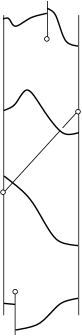
Figure 7.1. The vertical strip ${\mathcal{U}}$ minus rays $R_{\sigma}$ immerses isometrically in $S$.

Let ${\mathcal{U}}$ be the strip $[0,x_{0}]\times{\mathbb{R}}$ in ${\mathbb{R}}^{2}$, and let $v\subset{\mathcal{U}}$ be the line segment connecting $v_{-}=(0,0)$ to $v_{+}=(x_{0},y_{0})$. A neighborhood of $v$ in ${\mathcal{U}}$ embeds in $S$ by a local isometry that preserves horizontal and vertical directions. We can extend this to an isometric immersion $\psi:{\mathcal{U}}^{\prime}\to S$, where ${\mathcal{U}}^{\prime}$ has the following form: There is a discrete set $\widehat{\Sigma}\subset{\mathcal{U}}\setminus int(v)$, and for each $\sigma=(x,y)\in\widehat{\Sigma}$ a vertical ray $R_{\sigma}$ of the form $\{x\}\times(y,\infty)$ (“upward pointing”) or $\{x\}\times(-\infty,y)$ (“downward pointing”), so that the rays are pairwise disjoint, disjoint from $v$, and ${\mathcal{U}}^{\prime}={\mathcal{U}}\setminus\bigcup_{\sigma\in\widehat{\Sigma}}R_{\sigma}$ (see Figure 7.1). The map $\psi$ takes $\widehat{\Sigma}$ to $\Sigma$, and it is defined by extending the embedding at each $p\in v$ maximally along the vertical line through $p$ (in both directions) until the image encounters a singularity in $\Sigma$. (We include $v_{-}$ and $v_{+}$ in $\hat{\Sigma}$, and for these two points delete both an upward and a downward pointing ray.)

Let $\widehat{\gamma}$ be the preimage $\psi^{-1}(\gamma)$. This is a union of arcs properly embedded in ${\mathcal{U}}^{\prime}$, and transverse to the vertical foliation in ${\mathbb{R}}^{2}$. By definition of $c_{1}$ and $c_{2}$, each vertical line in ${\mathcal{U}}^{\prime}$ is cut by $\widehat{\gamma}$ into segments of length at least $c_{1}$ and at most $c_{2}$. Moreover the total vertical extent of each component of $\widehat{\gamma}$ is at most $c_{2}$.

Consider $\gamma_{1}$ the component of $\widehat{\gamma}$ that meets the downward ray based at $v_{+}$ at the highest point $\hat{r}$. The other endpoint $\hat{p}$ of $\gamma_{1}$ lies on some other ray $R_{\sigma}$.

The width of $\gamma_{1}$ is at most $x_{0}$, so the image points $r=\psi(\hat{r})$ and $p=\psi(\hat{p})$ satisfy $|p-r|\leq x_{0}$, with respect to the induced transverse measure on $\gamma$. We now check that $p$ and $r$ are images of discontinuity points of $\mathcal{T}$, by controlled powers of $\mathcal{T}$.

By choice of $\gamma_{1}$, the upward leaf emanating from $r$ encounters the singularity $\psi(v_{+})$ before it returns to $\gamma$, and hence $r$ itself is a discontinuity point $x_{i}$.

For $p$, Let us write $\sigma=(x,y)$ and $p=(x,y^{\prime})$. Suppose first that $y_{0}\geq 0$. There are now two cases. If $R_{\sigma}$ lies above $v$ (and hence is upward pointing): we have $y^{\prime}\geq y\geq 0$, and moreover (since the vertical variation of $\gamma_{1}$ is bounded) $y^{\prime}\leq y_{0}+c_{2}$. The segment of $R_{\sigma}$ between $\sigma$ and $p$ is cut by $\widehat{\gamma}$ (incident from the right) into at most $(y^{\prime}-y)/c_{1}$ pieces, and this implies that there is some $k\geq 0$ bounded by

$$k\leq\frac{y_{0}+c_{2}}{c_{1}}\leq\frac{e^{t/2}\phi+c_{2}}{c_{1}}$$

such that $p=T^{k}x_{j}$ for some discontinuity $x_{j}$.

If $R_{\sigma}$ lies below $v$ and is downward pointing: we have $y^{\prime}\leq y\leq y_{0}$ and $y^{\prime}\geq y_{0}-2c_{2}$, so that by the same logic there is $k\geq 0$ with

$$k\leq\frac{2c_{2}}{c_{1}}$$

such that $T^{k}p=x_{j}$ for some discontinuity $x_{j}$.

Hence in either case we have

$${|T^{m}x_{j}-x_{i}|\leq x_{0}\leq e^{-t/2}\phi}$$ (26)

where $-2c_{2}/c_{1}\leq m\leq(y_{0}+c_{2})/c_{1}$.

If $y_{0}<0$ there is a similar analysis, yielding the bound (26) where now $(y_{0}-2c_{2})/c_{1}\leq m\leq c_{2}/c_{1}$.

Noting that $\phi<1$ by area considerations, if we take $n=\lfloor\kappa e^{t/2}\rfloor$, where $\kappa=1+(1+2c_{2})/c_{1}$, then we guarantee $|m|\leq n$, and hence get

$$n\varepsilon_{n}\leq\kappa e^{t/2}e^{-t/2}\phi\leq\kappa\phi.$$

∎

8. Mahler’s question for lines

In this section we will derive Theorem 6.1 from Theorem 5.3 and earlier results of [KeMasSm, Mas2, KlWe1, KlWe2]. We will need the following:

Proposition 8.1.

For any $|\theta|<\pi/2$, there is a bounded subset $\Omega\subset G$ such that for any $t\geq 0$, and any $q\in{\mathcal{H}}$, there is $w\in\Omega$ such that $g_{t}h_{-\tan\theta}q=wg_{t}r_{\theta}q.$

Proof.

Let

$$x=\left(\begin{matrix}1/\cos\theta&0\\ -\sin\theta&\cos\theta\end{matrix}\right)\in G.$$

Then $g_{t}xg_{-t}$ converges in $G$ as $t\to\infty$, and we set $\Omega=\{g_{t}xg_{-t}:t\geq 0\}$. Since $xr_{\theta}=h_{-\tan\theta}$ and $g_{t}h_{-\tan\theta}q=g_{t}xr_{\theta}q=g_{t}xg_{-t}g_{t}r_{\theta}q$, the claim follows. ∎

Proof of Theorem 6.1.

Let $({\bf{a}},\mathbf{b})$ be positive, let ${\mathcal{U}}$ be a neighborhood of $({\bf{a}},\mathbf{b})$ in ${\mathbb{R}}^{d}_{+}\times{\mathbb{R}}^{d}$, let ${\mathbf{q}}:{\mathcal{U}}\to{\mathcal{H}}$ as in Theorem 5.3, let $q=\pi\circ{\mathbf{q}}$ where $\pi:\widetilde{\mathcal{H}}\to{\mathcal{H}}$ is the natural projection, and let $\varepsilon_{0}>0$ so that ${\bf{a}}(s)={\bf{a}}+s\mathbf{b}\in{\mathcal{U}}$ for all $s\in(-\varepsilon_{0},\varepsilon_{0})$. Making $\varepsilon_{0}$ smaller if necessary, let $\gamma$ be a judicious curve for $q$ such that $\mathcal{T}_{\sigma}({\bf{a}}(s))=\mathcal{T}(h_{s}q,\gamma)$ for all $s\in(-\varepsilon_{0},\varepsilon_{0})$. By Theorem 5.3 and Proposition 7.2, ${\bf{a}}(s)$ is of recurrence (resp. bounded) type if and only if there is a compact subset $K\subset{\mathcal{H}}$ such that $\{t>0:g_{t}h_{s}q\in K\}$ is unbounded (resp., is equal to $(0,\infty)$). The main result of [KeMasSm] is that for any $q$, for Lebesgue-a.e. $\theta\in(-\pi,\pi)$ there is a compact $K\subset{\mathcal{H}}$ such that $\{t>0:g_{t}r_{\theta}q\in K\}$ is unbounded. Thus (a) (with $\mu$ equal to Lebesgue measure) follows via Proposition 8.1. For a general measure $\mu$, the statement will follow from Corollary 9.3 below. Similarly (b) follows from [KlWe1] for $\mu$ equal to Lebesgue measure, and from [KlWe2] for a general decaying Federer measure, and (c) follows from [Mas2]. ∎

9. Quantitative nondivergence for horocycles

In this section we will recall a quantitative nondivergence result for the horocycle flow, which is a variant of results in [MiWe], and will be crucial for us. The theorem was stated without proof in [KlWe2, Prop. 8.3]. At the end of the section we will use it to obtain a strengthening of Theorem 6.1(a).

Given positive constants $C,\alpha,D$, we say that a regular finite Borel measure $\mu$ on ${\mathbb{R}}$ is $(C,\alpha)$-decaying and $D$-Federer if (21) holds for all $x\in{\mathrm{supp}}\,\mu$ and all $0<\varepsilon,r<1.$ For an interval $J=B(x,r)$ and $c>0$ we write $cJ=B(x,cr)$. Let ${\mathcal{H}}_{1}$ and $K_{\varepsilon}$ be as in §7, and let $\widetilde{\mathcal{H}}_{1}=\pi^{-1}({\mathcal{H}}_{1})$.

Theorem 9.1.

Given a stratum ${\mathcal{H}}$ of translation surfaces, there are positive constants $C_{1},\lambda,\rho_{0}$, such that for any $(C,\alpha)$-decaying and $D$-Federer measure $\mu$ on an interval $B\subset{\mathbb{R}}$, the following holds. Suppose $J\subset{\mathbb{R}}$ is an interval with $3J\subset B$, $0<\rho\leq\rho_{0},\,{\mathbf{q}}\in\widetilde{{\mathcal{H}}}_{1}$, and suppose

$${\forall\delta\in{\mathcal{L}}_{{\mathbf{q}}},\ \sup_{s\in J}\,\ell(\delta,h_{s}{\mathbf{q}})\geq\rho.}$$ (27)

Then for any $0<\varepsilon<\rho$:

$$\mu\left(\{s\in J:h_{s}\pi({\mathbf{q}})\notin K_{\varepsilon}\right\})\leq C^{\prime}\left(\frac{\varepsilon}{\rho}\right)^{\lambda\alpha}\mu(J),$$ (28)

where $C^{\prime}=C_{1}2^{\alpha}CD$.

Proof.

The proof is similar to that of [MiWe, Thm. 6.10], but with the assumption that $\mu$ is Federer substituting for condition (36) of that paper. To avoid repetition we give the proof making reference to [MiWe] when necessary.

Let $\lambda,\rho_{0},C_{1}$ substitute for $\gamma,\rho_{0},C$ as in [MiWe, Proof of Thm. 6.3]. For an interval $J\subset{\mathbb{R}}$, let $|J|$ denote its length. For a function $f:{\mathbb{R}}\to{\mathbb{R}}_{+}$ and $\varepsilon>0$, let

$$J_{f,\varepsilon}=\{x\in J:f(x)<\varepsilon\}\ \ \mathrm{and}\ \|f\|_{J}=\sup_{x\in J}f(x).$$

For $\delta\in{\mathcal{L}}_{\mathbf{q}}$ let $\ell_{\delta}$ be the function $\ell_{\delta}(s)=\ell(\delta,h_{s}{\mathbf{q}})$. Suppose, for ${\mathbf{q}}\in\widetilde{\mathcal{H}},\,\delta\in{\mathcal{L}}_{{\mathbf{q}}}$ and an interval $J$, that $\|\ell_{\delta}\|_{J}\geq\rho.$ An elementary computation (see [MiWe, Lemma 4.4]) shows that $J_{\varepsilon}=J_{\ell_{\delta},\varepsilon}$ is a subinterval of $J$ and

$$|J_{\varepsilon}|\leq\frac{2\varepsilon}{\rho}|J|.$$ (29)

Suppose that $\mu$ is $(C,\alpha)$-decaying and $D$-Federer, and ${\mathrm{supp}}\,\mu\cap J_{\varepsilon}\neq\varnothing$. Let $x\in{\mathrm{supp}}\,\mu\cap J_{\varepsilon}$. Note that $J_{\varepsilon}\subset B(x,|J_{\varepsilon}|)$ and $B(x,|J|)\subset 3J.$ One has

$$\begin{split}\mu(J_{\varepsilon})&\leq\mu(B(x,|J_{\varepsilon}|))\\ &\stackrel{{\scriptstyle\mathrm{decay,\ }\eqref{eq: ratio of lengths}}}{{\leq}}C\left(\frac{2\varepsilon}{\rho}\right)^{\alpha}\mu(B(x,|J|))\\ &\leq 2^{\alpha}C\left(\frac{\varepsilon}{\rho}\right)^{\alpha}\mu(3J)\leq C^{\prime\prime}\left(\frac{\varepsilon}{\rho}\right)^{\alpha}\mu(J),\end{split}$$

where $C^{\prime\prime}=2^{\alpha}CD$. This shows that if $J$ is an interval, ${\mathbf{q}}\in\widetilde{\mathcal{H}}$, and $\delta\in\mathcal{L}_{{\mathbf{q}}}$ is such that $\|\ell_{\delta}\|_{J}\geq\rho$, then for any $0<\varepsilon<\rho$,

$$\frac{\mu(J_{\ell_{\delta},\varepsilon})}{\mu(J)}\leq C^{\prime\prime}\left(\frac{\varepsilon}{\rho}\right)^{\alpha}.$$

Now to obtain (28), define $F(x)=C^{\prime\prime}x^{\alpha}$ and repeat the proof of [MiWe, Theorem 6.3], but using $\mu$ instead of Lebesgue measure on ${\mathbb{R}}$ and using [MiWe, Prop. 3.4] in place of [MiWe, Prop. 3.2]. ∎

Corollary 9.2.

For any stratum ${\mathcal{H}}$ of translation surfaces and any $C,\alpha,D$ there is a compact $K\subset{\mathcal{H}}_{1}$ such that for any $q\in{\mathcal{H}}_{1}$, any unbounded $\mathcal{T}\subset{\mathbb{R}}_{+}$ and any $(C,\alpha)$-decaying and $D$-Federer measure $\mu$ on an interval $J\subset{\mathbb{R}}$, for $\mu$-a.e. $s\in J$ there is a sequence $t_{n}\to\infty,\,t_{n}\in\mathcal{T}$ such that $g_{t_{n}}h_{s}q\in K$.

Proof.

Given $C,\alpha,D$, let $\lambda,\rho_{0},C^{\prime}$ be as in Theorem 9.1. Let $\varepsilon$ be small enough so that

$$C^{\prime}\left(\frac{\varepsilon}{\rho_{0}}\right)^{\lambda\alpha}<1,$$

and let $K=K_{\varepsilon}$. Suppose to the contrary that for some $(C,\alpha)$-decaying and $D$-Federer measure $\mu$ on some interval $J_{0}$ we have

$$\mu(A)>0,\ \ \mathrm{where}\ A=\{s\in J_{0}:\exists t_{0}\,\forall t\in\mathcal{T}\cap(t_{0},\infty),\,g_{t}h_{s}q\notin K\}.$$

Then there is $A_{0}\subset A$ and $t_{0}>0$ such that $\mu(A_{0})>0$ and

$${s\in A_{0},\ t\in\mathcal{T}\cap(t_{0},\infty)\ \implies\ g_{t}h_{s}q\notin K.}$$ (30)

By a general density theorem, see e.g. [Mat, Cor. 2.14], there is an interval $J$ with $3J\subset J_{0}$ such that

$${\frac{\mu(A_{0}\cap J)}{\mu(J)}>C^{\prime}\left(\frac{\varepsilon}{\rho_{0}}\right)^{\lambda\alpha}.}$$ (31)

We claim that by taking $t>t_{0}$ sufficiently large we can assume that for all $\delta\in{\mathcal{L}}_{{\mathbf{q}}}$ there is $s\in J$ such that $\ell(\delta,g_{t}h_{s}{\mathbf{q}})\geq\rho_{0}.$ This will guarantee that (27) holds for the horocycle $s\mapsto g_{t}h_{s}q=h_{e^{t}s}g_{t}q$, and conclude the proof since (30) and (31) contradict (28) (with $g_{t}q$ in place of $q$).

It remains to prove the claim. Let $\zeta=\phi(q)$ so that for any $\delta\in{\mathcal{L}}_{{\mathbf{q}}}$,

$$\ell(\delta,{\mathbf{q}})=\max\left\{|x(\delta,{\mathbf{q}})|,|y(\delta,{\mathbf{q}})|\right\}\geq\zeta.$$

If $|x(\delta,{\mathbf{q}})|\geq\zeta$, then $|x(\delta,g_{t}{\mathbf{q}})|=e^{t/2}|x(\delta,{\mathbf{q}})|\geq\zeta e^{t/2},$ and if $|y(\delta,{\mathbf{q}})|\geq\zeta$ then the function

$$s\mapsto x(\delta,g_{t}h_{s}{\mathbf{q}})=e^{t/2}\left(x(\delta,{\mathbf{q}})+sy(\delta,{\mathbf{q}})\right)$$

has slope $|e^{t/2}y(\delta,{\mathbf{q}})|\geq e^{t/2}\zeta$, hence $\sup_{s\in J}|x(\delta,g_{t}h_{s}{\mathbf{q}})|\geq\zeta e^{t/2}\frac{|J|}{2}.$ Thus the claim holds when $\zeta e^{t/2}\geq\max\left\{\rho_{0},\rho_{0}\frac{|J|}{2}\right\}.$ ∎

This yields a strengthening of Theorem 6.1(a).

Corollary 9.3.

Suppose $({\bf{a}},\mathbf{b})$ is positive, and write ${\bf{a}}(s)={\bf{a}}+s\mathbf{b}$. There is $\varepsilon_{0}>0$ such that given $C,\alpha,D$ there is $\zeta>0$ such that if $\mu$ is $(C,\alpha)$-decaying and $D$-Federer, and ${\mathrm{supp}}\,\mu\subset(-\varepsilon_{0},\varepsilon_{0})$, then for $\mu$-almost every $s$, $\limsup n\varepsilon_{n}({\bf{a}}(s))\geq\zeta.$

Proof.

Repeat the proof of Theorem 6.1, using Corollary 9.2 and Proposition 7.2 instead of [KeMasSm]. ∎

10. Mahler’s question for curves

In this section we prove Theorems 1.3 and 6.2 by deriving them from a stronger statement.

Theorem 10.1.

Let $J\subset{\mathbb{R}}$ be a compact interval, let $\beta:J\to{\mathbb{R}}^{d}_{+}$ be a $C^{2}$ curve, let $\mu$ be a decaying Federer measure on $J$, and suppose that for every $s_{1},s_{2}\in J$, $(\beta(s_{1}),\beta^{\prime}(s_{2}))$ is a positive pair. Then there is $\zeta>0$ such that for $\mu$-a.e. $s\in J,$ $\limsup_{n\to\infty}n\varepsilon_{n}(\beta(s))\geq\zeta$.

Derivation of Theorem 6.2 from Theorem 10.1.

If Theorem 6.2 is false then there is $A\subset I$ with $\mu(A)>0$ such that for all $s\in A$, $\beta(s)$ is not of recurrence type but $(\beta(s),\beta^{\prime}(s))$ is positive. Let $s_{0}\in A\cap{\mathrm{supp}}\,\mu$ so that $\mu(A\cap J)>0$ for any open interval $J$ containing $s_{0}$. Since the set of positive pairs is open (Corollary 5.4), there is an open $J$ containing $s_{0}$ such that $(\beta(s_{1}),\beta^{\prime}(s_{2}))$ is positive for every $s_{1},s_{2}\in J$, so Theorem 10.1 implies that $\beta(s)$ is of recurrence type for almost every $s\in J$, a contradiction. ∎

Proof of Theorem 1.3.

Let ${\bf{a}}(x)$ be as in (2) and let $\|\cdot\|_{1}$ be the 1-norm on ${\mathbb{R}}^{d}$. Since unique ergodicity is unaffected by dilations, it is enough to verify the conditions of Theorem 6.2 for the permutation $\sigma(i)=d+1-i$, a decaying Federer measure $\mu$, and for

$$\beta(s)=\frac{{\bf{a}}(s)}{\|{\bf{a}}(s)\|_{1}}=\frac{1}{s+\cdots+s^{d}}\left(s,s^{2},\ldots,s^{d}\right).$$

For any connection $(i,j,m)$ the set $\left\{{\bf{a}}\in\Delta:(i,j,m)\in{\mathcal{L}}_{\bf{a}}\right\}$ is a proper affine subspace of ${\mathbb{R}}^{d}_{+}$ transversal to $\{(x_{1},\ldots,x_{d}):\sum x_{i}=1\}$, and since $\beta(s)$ is analytic and not contained in any such affine subspace, the set $\{s\in I:\beta(s)\mathrm{\ has\ connections}\}$ is countable, so $\beta(s)$ is without connections for $\mu$-a.e. $s$.

Letting $R=R(s)=s+\cdots+s^{d}$, we have

$$\beta^{\prime}(s)=\frac{1}{R^{2}}\left(\gamma_{1}(s),\ldots,\gamma_{d}(s)\right),\ \ \ \mathrm{where}\ \ \gamma_{i}(s)=\sum_{\ell=i}^{i+d-1}\left(2i-\ell-1\right)s^{\ell}.$$

Then for $j=1,\ldots,d-1$ and $\ell=1,\ldots,j+d-1$, setting $a=\max\{1,\ell+1-d\},\,b=\min\{j,\ell\}$ we find:

$$\begin{split}R^{2}y_{j}&=\sum_{i=1}^{j}\gamma_{i}(s)=\sum_{\ell=1}^{j+d-1}\left(\sum_{i=a}^{b}(2i-\ell-1)\right)s^{\ell}\\ &=\sum_{\ell=1}^{j+d-1}\left[b(b+1)-a(a-1)-(b-a+1)(\ell+1)\right]s^{\ell}.\end{split}$$

Considering separately the 3 cases $1\leq\ell\leq j,\ j<\ell\leq d,\ d<\ell$ one sees that in every case $y_{j}<0$. Our choice of $\sigma$ insures that for $j=1,\ldots,d-1$, $y^{\prime}_{j}=-y_{d-j}>0$. This implies via (17) that $L<0$ on $I$, thus for all $s$ for which $\beta(s)$ is without connections, $\left(\beta(s),-\beta^{\prime}(s)\right)$ is positive. Define $\hat{\beta}(s)=\beta(-s)$, so that $\left(\hat{\beta}(s),\hat{\beta}^{\prime}(s)\right)=\left(\beta(-s),-\beta^{\prime}(-s)\right)$ is positive for a.e. $s<0$. Thus Theorem 6.2 applies to $\hat{\beta}$, proving the claim. ∎

Proof of Theorem 10.1.

Let ${\mathcal{H}}$ be the stratum corresponding to $\sigma$. For a $(C,\alpha)$-decaying and $D$-Federer measure $\mu$, let $C^{\prime},\rho_{0},\lambda$ be the constants as in Theorem 9.1. Choose $\varepsilon>0$ small enough so that

$${B=C^{\prime}\left(\frac{\varepsilon}{\rho_{0}}\right)^{\lambda\alpha}<1,}$$ (32)

and let $K=K_{\varepsilon}.$

By making $J$ smaller if necessary, we can assume that for all $s_{1},s_{2}\in J$, there is a translation surface $q(s_{1},s_{2})=\pi\circ{\mathbf{q}}(\beta(s_{1}),\beta^{\prime}(s_{2}))$ corresponding to the positive pair $(\beta(s_{1}),\beta^{\prime}(s_{2}))$ via Theorem 5.3. That is $Q=\{q(s_{1},s_{2}):s_{i}\in J\}$ is a bounded subset of ${\mathcal{H}}$ and $q(s_{1},s_{2})$ depends continuously on $s_{1},s_{2}$. By appealing to Corollary 5.5, we can also assume that there is a fixed curve $\gamma$ so that $\mathcal{T}_{\sigma}(\beta(s_{1}))=\mathcal{T}(q(s_{1},s_{2}),\gamma),$ for $s_{1},s_{2}\in J$. Define $q(s)=q(s,s)$. By rescaling we may assume with no loss of generality that $q(s)\in{\mathcal{H}}_{1}$ for all $s$, and by making $K$ larger let us assume that $Q\subset K.$ By continuity, the return times to $\gamma$ along vertical leaves for $q(s_{1},s_{2})$ are uniformly bounded from above and below, and the length of $\gamma$ with respect to the flat structure given by $q(s_{1},s_{2})$ is uniformly bounded.

We claim that there is $C_{1}$, depending only on $Q$, such that for any interval $J_{0}\subset{\mathbb{R}}$ with $0\in J_{0}$, any $t>0$, any $q\in Q$, any ${\mathbf{q}}\in\pi^{-1}(q)$ and any $\delta\in{\mathcal{L}}_{{\mathbf{q}}}$, we have

$$\sup_{s\in J_{0}}\ell(\delta,g_{t}h_{s}{\mathbf{q}})\geq C_{1}|J_{0}|e^{t/2}.$$

Here $|J_{0}|$ is the length of $J_{0}$.

Indeed, let $\theta=\inf\{\phi(q):q\in Q\},$ which is a positive number since $Q$ is bounded. Let $C_{1}=\min\left\{\frac{\theta}{|J_{0}|},\frac{\theta}{2}\right\}$, and let $q\in Q,\,{\mathbf{q}}\in\pi^{-1}(q),\,\delta\in{\mathcal{L}}_{{\mathbf{q}}}$. Then $\max\left\{|x(\delta,{\mathbf{q}})|,|y(\delta,{\mathbf{q}})|\right\}\geq\theta.$ Suppose first that $|x(\delta,{\mathbf{q}})|\geq\theta$, then

$$\sup_{s\in J_{0}}\ell(\delta,g_{t}h_{s}{\mathbf{q}})\geq|x(\delta,g_{t}{\mathbf{q}})|=e^{t/2}|x(\delta,{\mathbf{q}})|\geq\theta e^{t/2}\geq C_{1}|J_{0}|e^{t/2}.$$

Now if $|y(\delta,{\mathbf{q}})|\geq\theta$ then the function

$$s\mapsto x(\delta,g_{t}h_{s}{\mathbf{q}})=e^{t/2}\left(x(\delta,{\mathbf{q}})+sy(\delta,{\mathbf{q}})\right)$$

has slope $|e^{t/2}y(\delta,{\mathbf{q}})|\geq e^{t/2}\theta$, hence

$$\sup_{s\in J_{0}}\ell(\delta,g_{t}h_{s}{\mathbf{q}})\geq\sup_{s\in J_{0}}|x(\delta,g_{t}h_{s}{\mathbf{q}})|\geq e^{t/2}\theta|J_{0}|/2\geq C_{1}|J_{0}|e^{t/2}.$$

This proves the claim.

For each $s_{0},s\in J$ let ${\bf{a}}^{(s_{0})}(s)=\beta(s_{0})+\beta^{\prime}(s_{0})(s-s_{0})$ be the linear approximation to $\beta$ at $s_{0}$. Using the fact that $\beta$ is a $C^{2}$-map, there is $\widetilde{C}$ such that

$${\max_{s\in J_{0}}\|\beta(s)-{\bf{a}}^{(s_{0})}(s)\|<\widetilde{C}|J_{0}|^{2}}$$ (33)

whenever $J_{0}\subset J$ is a subinterval centered at $s_{0}$.

Let $\kappa$ and $c_{2}$ be as in Proposition 7.2, let $\varepsilon$ be as chosen in (32), let

$$C_{2}=\frac{\rho_{0}}{2C_{1}},\ \ \ \zeta_{1}<\left(\frac{\varepsilon}{\kappa}\right)^{2}\ \ \ \mathrm{and}\ \ \zeta=\zeta_{1}\cdot\frac{c_{2}}{d^{2}\widetilde{C}}.$$

If the theorem is false then $\mu(A)>0$, where

$$A=\{s\in J:\limsup n\varepsilon_{n}(\beta(s))<\zeta\}.$$

Moreover there is $N$ and $A_{0}\subset A$ such that $\mu(A_{0})>0$ and

$${n\geq N,\,s\in A_{0}\ \implies\ n\varepsilon_{n}(\beta(s))<\zeta.}$$ (34)

Using [Mat, Cor. 2.14] let $s_{0}\in A_{0}$ be a density point, so that for any sufficiently small interval $J_{0}$ centered at $s_{0}$ we have

$${\mu(A_{0}\cap J_{0})>B\mu(J_{0}),}$$ (35)

where $B$ is as in (32).

For $t>0$ we will write

$$c(t)=C_{2}e^{-t/2}\ \ \ \mathrm{and}\ \ \ J_{t}=B(s_{0},c(t)).$$

Let ${\bf{a}}(s)={\bf{a}}^{(s_{0})}(s)$ and let $\widetilde{q}(s)=h_{s-s_{0}}q(s_{0})$, which is the surface $\pi\circ{\mathbf{q}}({\bf{a}}(s),\beta^{\prime}(s_{0}))$. The trajectory $s\mapsto g_{t}\widetilde{q}(s)=g_{t}h_{s-s_{0}}q(s_{0})=h_{e^{t}s}g_{t}h_{-s_{0}}q(s_{0})$ is a horocycle path, which, by the claim and the choice of $C_{2}$, satisfies (27) with $\rho=\rho_{0}$ and $J=J_{t}$ for all $t>0$. Therefore

$${\mu\left\{s\in J_{t}:g_{t}\widetilde{q}(s)\notin K\right\}\leq B\mu(J_{t}).}$$ (36)

Now for a large $t>0$ to be specified below, let

$${n_{1}=\sqrt{\frac{\zeta_{1}}{2c_{2}}}e^{t/2}\ \ \ \mathrm{and}\ \ n_{2}=\frac{2c_{2}}{d^{2}\widetilde{C}}n_{1}.}$$ (37)

By making $\widetilde{C}$ larger we can assume that $n_{2}<n_{1}$. For large enough $t$ we will have $n_{2}>n_{0}$ (as in Proposition 7.2) and $n_{2}>N$ (as in (34)).

We now claim

$${s\in J_{t},\ n_{2}\varepsilon_{n_{2}}(\beta(s))<\zeta\ \implies\ n_{1}\varepsilon_{n_{1}}({\bf{a}}(s))<\zeta_{1}.}$$ (38)

Assuming this, note that by (23), (37) and the choice of $\zeta_{1}$, if $n_{1}\varepsilon_{n_{1}}({\bf{a}}(s))<\zeta_{1}$ then $g_{t}\widetilde{q}(s)\notin K$. Combining (34) and (38) we see that $A_{0}\cap J_{t}\subset\{s\in J_{t}:g_{t}\widetilde{q}(s)\notin K\}$ for all large enough $t$. Combining this with (35) we find a contradiction to (36).

It remains to prove (38). Let $r\leq n_{2}$, let $\mathcal{T}=\mathcal{T}_{\sigma}({\bf{a}}(s)),\ {\mathcal{S}}=\mathcal{T}_{\sigma}(\beta(s))$, let $x_{i},x_{j}$ be discontinuities of $\mathcal{T}$ and let $x^{\prime}_{i},x^{\prime}_{j}$ be the corresponding discontinuities of ${\mathcal{S}}$. By choice of $\widetilde{C}$ we have

$$\|\beta(s)-{\bf{a}}(s)\|<\widetilde{C}e^{-t},$$

where $\|\cdot\|$ is the max norm on ${\mathbb{R}}^{d}$. Suppose first that $x_{i}$ and $x^{\prime}_{i}$ have the same itinerary under $\mathcal{T}$ and ${\mathcal{S}}$ until the $r$th iteration; i.e. $\mathcal{T}^{k}x_{i}$ is in the $\ell$th interval of continuity of $\mathcal{T}$ if and only if ${\mathcal{S}}^{k}x^{\prime}_{i}$ is in the $\ell$th interval of continuity of ${\mathcal{S}}$ for $k\leq r$. Then one sees from (8) and (9) that

$$|\mathcal{T}^{r}x_{i}-{\mathcal{S}}^{r}x^{\prime}_{i}|\leq\sum_{0}^{r}d^{2}\|\beta(s)-{\bf{a}}(s)\|.$$

Therefore, using (37),

$$\begin{split}\left|x_{i}-\mathcal{T}^{r}x_{j}-(x^{\prime}_{i}-{\mathcal{S}}^{r}x^{\prime}_{j})\right|&\leq\left|x_{i}-x^{\prime}_{i}\right|+\left|\mathcal{T}^{r}x_{j}-{\mathcal{S}}^{r}x^{\prime}_{j}\right|\\ &\leq 2\sum_{1}^{r}d^{2}\|\beta(s)-{\bf{a}}(s)\|\\ &\leq 2d^{2}n_{2}\widetilde{C}e^{-t}=\frac{\zeta_{1}}{2n_{1}}.\end{split}$$

If $n_{1}\varepsilon_{n_{1}}({\bf{a}}(s))\geq\zeta_{1}$ then by the triangle inequality we find that $|x^{\prime}_{i}-{\mathcal{S}}^{r}x^{\prime}_{j}|<\zeta_{1}/2n_{1}>0$. In particular this shows that for all $i$, $x_{i}$ and $x^{\prime}_{i}$ do have the same itinerary under $\mathcal{T}$ and ${\mathcal{S}}$, and moreover

$$\begin{split}\varepsilon_{n_{2}}(\beta(s))&\geq\varepsilon_{n_{2}}({\bf{a}}(s))-\frac{\zeta_{1}}{2n_{1}}\\ &\geq\varepsilon_{n_{1}}({\bf{a}}(s))-\frac{\zeta_{1}}{2n_{1}}\\ &>\frac{\zeta_{1}}{2n_{1}}=\zeta_{1}\frac{n_{2}}{2n_{1}}\cdot\frac{1}{n_{2}}=\frac{\zeta}{n_{2}},\end{split}$$

as required. ∎

11. Real REL

This section contains our results concerning the real REL foliation, whose definition we now recall. Let ${\mathbf{q}}$ be a marked translation surface of type ${\mathbf{r}}$, where $k$ (the number of singularities) is at least 2. Recall that ${\mathbf{q}}$ determines a cohomology class ${\mathrm{hol}}({\mathbf{q}})$ in $H^{1}(S,\Sigma;{\mathbb{R}}^{2})$, where for a relative cycle $\gamma\in H_{1}(S,\Sigma),$ the value ${\mathbf{q}}$ takes on $\gamma$ is ${\mathrm{hol}}(\gamma,{\mathbf{q}})$. Also recall that there are open sets $\widetilde{\mathcal{H}}_{\tau}$ in $\widetilde{\mathcal{H}}({\mathbf{r}})$, corresponding to a given triangulation of $(S,\Sigma)$, such that the map hol restricted to $\widetilde{\mathcal{H}}_{\tau}$ endows $\widetilde{\mathcal{H}}$ with a linear manifold structure. Now recall the map Res as in (4), let $V_{1}$ be the first summand in the splitting (3), and let $W=V_{1}\cap\ker\,\operatorname{Res},$ so that $\dim W=k-1,$ where $k=|\Sigma|$. The REL foliation is modeled on $\ker\,\operatorname{Res}$, the real foliation is modeled on $V_{1}$, and the real REL foliation is modeled on $W$. That is, a ball $\mathcal{U}\subset\widetilde{\mathcal{H}}_{\tau}$ provides a product neighborhood for these foliations, where ${\mathbf{q}},{\mathbf{q}}_{1}\in\mathcal{U}$ belong to the same plaque for REL, real, or real REL, if ${\mathrm{hol}}({\mathbf{q}})-{\mathrm{hol}}({\mathbf{q}}_{1})$ belongs respectively to $\ker\operatorname{Res},V_{1},$ or $W$.

Recall that ${\mathcal{H}}$ is an orbifold and the orbifold cover $\pi:\widetilde{\mathcal{H}}\to{\mathcal{H}}$ is defined by taking a quotient by the $\operatorname{Mod}(S,\Sigma)$-action. Since hol is equivariant with respect to the action of the group $\operatorname{Mod}(S,\Sigma)$ on $\widetilde{\mathcal{H}}$ and $H^{1}(S,\Sigma;{\mathbb{R}}^{2})$, and (by naturality of the splitting (3) and the sequence (4)) the subspaces $V_{1},W,$ and $\ker\,\operatorname{Res}$ are $\operatorname{Mod}(S,\Sigma)$-invariant, the foliations defined by these subspaces on $\widetilde{\mathcal{H}}$ descend naturally to ${\mathcal{H}}$. More precisely leaves in $\widetilde{\mathcal{H}}$ descend to ‘orbifold leaves’ on ${\mathcal{H}}$, i.e. leaves in $\widetilde{\mathcal{H}}$ map to immersed sub-orbifolds in ${\mathcal{H}}$. In order to avoid dealing with orbifold foliations, we pass to a finite cover $\hat{{\mathcal{H}}}\to{\mathcal{H}}$ which is a manifold, as explained in §2.1.

Proposition 11.1.

The REL and real REL leaves on both $\widetilde{\mathcal{H}}$ and $\hat{\mathcal{H}}$ have a well-defined translation structure.

Proof.

A translation structure on a leaf $\mathcal{L}$ amounts to saying that there is a fixed vector space $V$ and an atlas of charts on $\mathcal{L}$ taking values in $V$, so that transition maps are translations. We take $V=\ker\,\operatorname{Res}$ for the REL leaves, and $V=W$ for the real REL leaves. For each ${\mathbf{q}}_{0}\in\widetilde{\mathcal{H}}$, the atlas is obtained by taking the chart ${\mathbf{q}}\mapsto{\mathrm{hol}}({\mathbf{q}})-{\mathrm{hol}}({\mathbf{q}}_{0})$. By the definition of the corresponding foliations, these are homeomorphisms in a sufficiently small neighborhood of ${\mathbf{q}}_{0}$, and the fact that transition maps are translations is immediate. In order to check that this descends to $\hat{\mathcal{H}}$, let $\Lambda\subset\operatorname{Mod}(S,\Sigma)$ be the finite-index torsion free subgroup so that $\hat{\mathcal{H}}=\widetilde{\mathcal{H}}/\Lambda$, and let $\varphi\in\Lambda$. We need to show that if $\hat{{\mathbf{q}}}={\mathbf{q}}\circ\varphi,\ \hat{{\mathbf{q}}}_{0}={\mathbf{q}}_{0}\circ\varphi,$ then ${\mathrm{hol}}({\mathbf{q}})-{\mathrm{hol}}({\mathbf{q}}_{0})={\mathrm{hol}}(\hat{{\mathbf{q}}})-{\mathrm{hol}}(\hat{{\mathbf{q}}}_{0})$. Since ${\mathrm{hol}}$ is $\operatorname{Mod}(S,\Sigma)$-equivariant, this amounts to checking that $\varphi$ acts trivially on $\ker\,\operatorname{Res}$. Invoking (4), this follows from our convention that any $\varphi\in\operatorname{Mod}(S,\Sigma)$ fixes each point of $\Sigma$, so acts trivially on $H^{0}(\Sigma)$. ∎

It is an interesting question to understand the geometry of individual leaves. For the REL foliation this is a challenging problem, but for the real REL foliation, our main theorems give a complete answer. Given a marked translation surface ${\mathbf{q}}$ we say that a saddle connection $\delta$ for ${\mathbf{q}}$ is horizontal if $y({\mathbf{q}},\delta)=0$. Note that for a generic ${\mathbf{q}}$ there are no horizontal saddle connections, and in any stratum there is a uniform upper bound on their number.

Theorem 11.2.

Let ${\mathbf{q}}\in\widetilde{\mathcal{H}}$ and let $\mathcal{V}\subset W$ such that for any $\mathbf{c}\in\mathcal{V}$ there is a path $\left\{\mathbf{c}_{t}\right\}_{t\in[0,1]}$ in $\mathcal{V}$ from 0 to $\mathbf{c}$ such that for any horizontal saddle connection for ${\mathbf{q}}$ and any $t\in[0,1]$, ${\mathrm{hol}}({\mathbf{q}},\delta)+\mathbf{c}_{t}(\delta)\neq 0$. Then there is a continuous map $\psi:\mathcal{V}\to\widetilde{\mathcal{H}}$ such that for any $\mathbf{c}\in\mathcal{V}$,

$${{\mathrm{hol}}(\psi(\mathbf{c}))={\mathrm{hol}}({\mathbf{q}})+(\mathbf{c},0),}$$ (39)

and the horizontal foliations of $\psi(\mathbf{c})$ is the same as that of ${\mathbf{q}}$. Moreover the image of $\psi$ is contained in the REL leaf of ${\mathbf{q}}$.

Proof.

Let ${\mathcal{F}}$ and ${\mathcal{G}}$ be the vertical and horizontal foliations of ${\mathbf{q}}$ respectively. We will apply Theorem 1.2, reversing the roles of the horizontal and vertical foliations of ${\mathbf{q}}$; that is we use ${\mathcal{G}}$ in place of ${\mathcal{F}}$. To do this, we will check that the map which sends $\mathbf{c}\in\mathcal{V}$ to $(x({\mathbf{q}})+\mathbf{c},y({\mathbf{q}}))\in H^{1}(S,\Sigma)^{2}$ has its image in $\mathbb{B}({\mathcal{G}})\times\mathbb{A}({\mathcal{G}})$ (notation as in Theorem 1.2), and thus

$$\psi(\mathbf{c})={\mathrm{hol}}^{-1}(x({\mathbf{q}})+\mathbf{c},y({\mathbf{q}}))$$

is continuous and satisfies (39).

Clearly $y({\mathbf{q}})$, the cohomology class represented by ${\mathcal{G}}$, is in $\mathbb{A}({\mathcal{G}})$. To check that $x({\mathbf{q}})+\mathbf{c}\in\mathbb{B}({\mathcal{G}})$, we need to show that for any element $\delta\in H^{\mathcal{G}}_{+}$, $x({\mathbf{q}},\delta)+\mathbf{c}(\delta)>0$. To see this, we treat separately the cases when $\delta$ is a horizontal saddle connection, and when $\delta$ is represented by a foliation cycle, i.e. an element of $H_{1}(S,\Sigma)$ which is in the image of $H_{1}(S)$ (and belongs to the convex cone spanned by the asymptotic cycles). If $\delta$ is a foliation cycle, since $\mathbf{c}\in W\subset\ker\,\mathrm{Res}$, the easy direction in Theorem 1.1 implies

$$x({\mathbf{q}},\delta)+\mathbf{c}(\delta)=x({\mathbf{q}},\delta)>0.$$

If $\delta$ is represented by a saddle connection, let $\{\mathbf{c}_{t}\}$ be a path from 0 to $\mathbf{c}$ in $\mathcal{V}$. Again, by the easy direction in Theorem 1.1, $x({\mathbf{q}},\delta)>0$, and the function $x({\mathbf{q}},\delta)+\mathbf{c}_{t}(\delta)$ is a continuous function of $t$, which does not vanish by hypothesis. This implies again that $x({\mathbf{q}},\delta)+\mathbf{c}(\delta)>0$.

To check $\psi(\mathbf{c})$ is contained in the real REL leaf of ${\mathbf{q}}$, it suffices to note that according to (39), in any local chart provided by hol, $\psi(\mathbf{c}_{t})$ moves along plaques of the foliation. ∎

Since the leaves are modelled on $W$, taking $\mathcal{V}=W$ we obtain:

Corollary 11.3.

If ${\mathbf{q}}$ has no horizontal saddle connections, then there is a homeomorphism $\psi:W\to\widetilde{\mathcal{H}}$ onto the leaf of ${\mathbf{q}}$.

Moreover the above maps are compatible with the transverse structure for the real REL foliation. Namely, let $\psi_{\mathbf{q}}$ be the map in Theorem 11.2. We have:

Corollary 11.4.

For any ${\mathbf{q}}_{0}\in\widetilde{\mathcal{H}}$ there is a neighborhood $\mathcal{V}$ of 0 in $W$, and a submanifold $\mathcal{U}^{\prime}\subset\widetilde{\mathcal{H}}$ everywhere transverse to real-REL leaves and containing ${\mathbf{q}}_{0}$ such that:

1. For any ${\mathbf{q}}\in\mathcal{U}^{\prime}$, $\psi_{{\mathbf{q}}}$ is defined on $\mathcal{V}$.

2. The map $\mathcal{U}^{\prime}\times\mathcal{V}$ defined by $({\mathbf{q}},\mathbf{c})\mapsto\psi_{{\mathbf{q}}}(\mathbf{c})$ is a homeomorphism onto its image, which is a neighborhood $\mathcal{U}$ of ${\mathbf{q}}_{0}$.

3. Each plaque of the real REL foliation in $\mathcal{U}$ is of the form $\psi_{{\mathbf{q}}}(\mathcal{V})$.

Proof.

Let $\mathcal{U}_{0}$ be a bounded neighborhood of ${\mathbf{q}}_{0}$ on which hol is a local homeomorphism and let $\mathcal{U}^{\prime}\subset\mathcal{U}_{0}$ be any submanifold everywhere transverse to the real REL leaves and of complementary dimension. For example we can take $\mathcal{U}^{\prime}$ to be the pre-image under hol of a small ball around ${\mathrm{hol}}({\mathbf{q}}_{0})$ in an affine subspace of $H^{1}(S,\Sigma;{\mathbb{R}}^{2})$ which is complementary to $W$.

Since $\mathcal{U}_{0}$ is bounded there is a uniform lower bound $r$ on the lengths of saddle connections for ${\mathbf{q}}\in\mathcal{U}_{0}$. If we let $\mathcal{V}_{0}$ be the ball of radius $r/2$ around 0 in $W$, then the conditions of Theorem 11.2 are satisfied for $\mathcal{V}_{0}$ and any ${\mathbf{q}}\in\mathcal{U}^{\prime}$. Thus (1) holds for any $\mathcal{V}\subset\mathcal{V}_{0}$. Taking for $\mathcal{V}$ a small ball around 0 we can assume that $\Psi_{{\mathbf{q}}}(\mathcal{V})\subset\mathcal{U}_{0}$ for any ${\mathbf{q}}$. From (39) and the choice of $\mathcal{U}^{\prime}$ it follows that $\{\psi_{{\mathbf{q}}}(\mathbf{c}):{\mathbf{q}}\in\mathcal{U}^{\prime},\mathbf{c}\in\mathcal{V}\}$ is a neighborhood of ${\mathrm{hol}}({\mathbf{q}}_{0})$ in $H^{1}(S,\Sigma;{\mathbb{R}}^{2})$. Assertions (2),(3) now follow from the fact that ${\mathrm{hol}}|_{\mathcal{U}_{0}}$ is a homeomorphism. ∎

Proof of Theorem 1.4.

Let $\hat{{\mathcal{H}}},\,\widetilde{\mathcal{H}}$ be as above, let $\pi:\widetilde{\mathcal{H}}\to\hat{{\mathcal{H}}}$ be the projection, let $\widetilde{Q}$ denote the subset of translation surfaces in $\widetilde{{\mathcal{H}}}$ without horizontal saddle connections, and let $Q=\pi(\widetilde{Q})$. Note that $Q$ and $\widetilde{Q}$ are $B$-invariant, where $B$ is the subgroup of upper triangular matrices in $G$, acting on $\hat{{\mathcal{H}}},\,\widetilde{\mathcal{H}}$ in the usual way. We will extend the $B$-action to an action of $F=B\ltimes W$.

The action of $W$ is defined as follows. For each ${\mathbf{q}}\in\widetilde{Q}$, the conditions of Theorem 11.2 are vacuously satisfied for $\mathcal{V}=W$, and we define $\mathbf{c}{\mathbf{q}}=\psi_{{\mathbf{q}}}(\mathbf{c})$. We first prove the group action law

$${(\mathbf{c}_{1}+\mathbf{c}_{2}){\mathbf{q}}=\mathbf{c}_{1}(\mathbf{c}_{2}{\mathbf{q}})}$$ (40)

for the action of $W$. This follows from (39), associativity of addition in $H^{1}(S,\Sigma;{\mathbb{R}}^{2})$, and the uniqueness in Lemma 4.1. Thus we have defined an action of $W$ on $\widetilde{Q}$, and by Proposition 11.1 this descends to a well-defined action on $Q$. To see that the action map $W\times\widetilde{Q}\to\widetilde{Q}$ is continuous, we take $w_{n}\to w$ in $W$, ${\mathbf{q}}^{(n)}\to{\mathbf{q}}$ in $\widetilde{Q}$, and need to show that

$${w_{n}{\mathbf{q}}^{(n)}\to w{\mathbf{q}}.}$$ (41)

Corollary 11.4 implies that for any $t$ there are neighborhoods $\mathcal{U}$ of $(tw){\mathbf{q}}$ and $\mathcal{V}$ of 0 in $W$ such that the map

$$\mathcal{U}\times\mathcal{V}\to\widetilde{\mathcal{H}},\ \ ({\mathbf{q}},\mathbf{c})\mapsto\mathbf{c}{\mathbf{q}}$$

is continuous. By compactness we can find $\mathcal{U}_{i},i=1,\ldots,k$, a partition $0=t_{0}<\cdots<t_{k}=1$, and a fixed open $\mathcal{V}\subset W$ such that

• $\{(tw){\mathbf{q}}:t\in[t_{i-1},t_{i}]\}\subset\mathcal{U}_{i}$.

• $(t_{i}-t_{i-1})w\in\mathcal{V}$.

It now follows by induction on $i$ that $t_{i}w^{(n)}{\mathbf{q}}_{n}\to(t_{i}w){\mathbf{q}}$ for each $i$, and putting $i=k$ we get (41).

The action is affine and measure preserving since in the local charts given by $H^{1}(S,\Sigma;{\mathbb{R}}^{2})$, it is defined by vector addition. Since the area of a surface can be computed in terms of its absolute periods alone, this action preserves the subset of area-one surfaces. A simple calculation using (7) shows that for ${\mathbf{q}}\in\widetilde{Q},\,\mathbf{c}\in W$ and

$$g=\left(\begin{matrix}a&b\\ 0&a^{-1}\end{matrix}\right)\in B,$$

we have $g\mathbf{c}{\mathbf{q}}=(a\mathbf{c})g{\mathbf{q}}$. That is, the actions of $B$ and $W$ respect the commutation relation defining $F$, so that we have defined an $F$-action on $\widetilde{Q}$. To check continuity of the action, let $f_{n}\to f$ in $F$ and ${\mathbf{q}}_{n}\to{\mathbf{q}}\in\widetilde{Q}$. Since $F$ is a semi-direct product we can write $f_{n}=w_{n}b_{n}$, where $w_{n}\to w$ in $W$ and $b_{n}\to b$ in $B$. Since the $B$-action is continuous, $b_{n}{\mathbf{q}}_{n}\to b{\mathbf{q}}$, and since (as verified above) the $W$-action on $\widetilde{Q}$ is continuous,

$$f_{n}{\mathbf{q}}_{n}=w_{n}(b_{n}{\mathbf{q}}_{n})\to w(b{\mathbf{q}})=f{\mathbf{q}}.$$

∎

12. Cones of good directions

Suppose $\sigma$ is an irreducible and admissible permutation, and let

$${{\mathcal{C}}_{{\bf{a}}}=\{\mathbf{b}\in{\mathbb{R}}^{d}:({\bf{a}},\mathbf{b})\mathrm{\ is\ positive}\}\subset T_{{\bf{a}}}{\mathbb{R}}^{d}_{+}.}$$ (42)

As we showed in Corollary 5.5, this is the set of good directions at the tangent space of ${\bf{a}}$, i.e. the directions of lines which may be lifted to horocycles. In this section we will relate the cones ${\mathcal{C}}_{{\bf{a}}}$ with the bilinear form $Q$ as in (10), and show there are ‘universally good’ directions for $\sigma$, i.e. specify certain $\mathbf{b}$ such that $\mathbf{b}\in{\mathcal{C}}_{\bf{a}}$ for all ${\bf{a}}$ which are without connections. We will also find ‘universally bad’ directions, i.e. directions which do not belong to ${\mathcal{C}}_{{\bf{a}}}$ for any ${\bf{a}}$; these will be seen to be related to real REL.

Set ${\mathcal{C}}_{{\bf{a}}}^{+}=\{\mathbf{b}\in{\mathbb{R}}^{d}:\mathrm{\eqref{eq: positivity}\ holds}\}$, so that ${\mathcal{C}}_{{\bf{a}}}\subset{\mathcal{C}}_{{\bf{a}}}^{+}$ for all ${\bf{a}}$, and ${\mathcal{C}}_{{\bf{a}}}^{+}={\mathcal{C}}_{{\bf{a}}}$ when ${\bf{a}}$ has no connections. Now let

$${{\mathcal{C}}=\left\{\mathbf{b}\in{\mathbb{R}}^{d}:\forall i,\,Q({\mathbf{e}}_{i},\mathbf{b})>0\right\}.}$$ (43)

We have:

Proposition 12.1.

${\mathcal{C}}$ is a nonempty open convex cone, and ${\mathcal{C}}=\bigcap_{{\bf{a}}}{\mathcal{C}}_{{\bf{a}}}^{+}.$

Proof.

It is clear that ${\mathcal{C}}$ is open and convex. It follows from (18) that

$${\mathcal{C}}=\left\{\mathbf{b}\in{\mathbb{R}}^{d}:\forall x\in I,\,\forall{\bf{a}}\in{\mathbb{R}}^{d}_{+},\,L_{{\bf{a}},\mathbf{b}}(x)>0\right\}.$$

The irreducibility of $\sigma$ implies that $\mathbf{b}_{0}=(b_{1},\ldots,b_{d})$ defined by $b_{i}=\sigma(i)-i$ (as in [Mas1]) satisfies $y_{i}(\mathbf{b}_{0})>0>y^{\prime}_{i}(\mathbf{b}_{0})$ for all $i$, so by (17), $L_{{\bf{a}},\mathbf{b}_{0}}$ is everywhere positive irrespective of ${\bf{a}}$. This shows that $\mathbf{b}_{0}$ belongs to ${\mathcal{C}}$, and moreover that ${\mathcal{C}}$ is contained in ${\mathcal{C}}^{+}_{{\bf{a}}}$ for any ${\bf{a}}$.

For the inclusion $\bigcap_{{\bf{a}}}{\mathcal{C}}^{+}_{{\bf{a}}}\subset{\mathcal{C}}$, suppose $\mathbf{b}\notin{\mathcal{C}}_{{\bf{a}}}^{+}$, so that for some $\mu\in{\mathcal{M}}_{{\bf{a}}}$ we have $\int L\,d\mu\leq 0.$ Writing ${\bf{a}}^{\prime}=(a^{\prime}_{1},\ldots,a^{\prime}_{d})$, where $a^{\prime}_{j}=\mu(I_{j})$, we have

$$Q({\bf{a}}^{\prime},\mathbf{b})=\sum a^{\prime}_{i}Q({\mathbf{e}}_{i},\mathbf{b})=\int L\,d\mu\leq 0,$$

so that $\mathbf{b}\notin{\mathcal{C}}.$ ∎

Note that in the course of the proof of Theorem 1.3, we actually showed that ${\bf{a}}^{\prime}(s)\in-{\mathcal{C}}$ for all $s>0$. Indeed, given a curve $\{\alpha(s)\}\subset{\mathbb{R}}^{d}_{+}$, the easiest way to show that $\alpha(s)$ is uniquely ergodic for a.e. $s$, is to show that $\alpha^{\prime}(s)\in\pm{\mathcal{C}}$ for a.e. $s$.

Let $\mathbf{R}$ denote the null-space of $Q$, that is

$$\mathbf{R}=\{\mathbf{b}\in{\mathbb{R}}^{d}:Q(\cdot,\mathbf{b})\equiv 0\}.$$

Proposition 12.2.

$\mathbf{R}={\mathbb{R}}^{d}\smallsetminus\bigcup_{{\bf{a}}}\pm{\mathcal{C}}_{{\bf{a}}}.$

Proof.

By (18), $\mathbf{R}=\{\mathbf{b}\in{\mathbb{R}}^{d}:L_{{\bf{a}},\mathbf{b}}(x)\equiv 0\},$ so that containment $\subset$ is clear. Now suppose $\mathbf{b}\notin\mathbf{R}$, that is $Q({\mathbf{e}}_{i},\mathbf{b})\neq 0$ for some $i$, and by continuity there is an open subset $\mathcal{U}$ of ${\mathbb{R}}^{d}_{+}$ such that $Q({\bf{a}},\mathbf{b})\neq 0$ for ${\bf{a}}\in\mathcal{U}$. Now taking ${\bf{a}}\in\mathcal{U}$ which is uniquely ergodic and without connections we have $\mathbf{b}\in\pm{\mathcal{C}}_{{\bf{a}}}.$ ∎

Consider the map $({\bf{a}},\mathbf{b})\mapsto{\mathbf{q}}({\bf{a}},\mathbf{b})$ defined in Theorem 5.3. It is easy to see that the image of an open subset of ${\mathbb{R}}^{d}_{+}\times\{\mathbf{b}\}$ is a plaque for the real foliation. Additionally, recalling that $Q({\bf{a}},\mathbf{b})$ records the intersection pairing on $H_{1}(S,\Sigma)\times H_{1}(S\smallsetminus\Sigma)$, and that the intersection pairing gives the duality $H_{1}(S\smallsetminus\Sigma)\cong H^{1}(S,\Sigma)$, one finds that the image of $\mathbf{R}\times\{\mathbf{b}\}$ is a plaque for the real REL foliation. That is, Proposition 12.2 says that the tangent directions in $T{\mathbb{R}}^{d}_{+}$ which can never be realized as horocycle directions, are precisely the directions in the real REL leaf.

References

- [Bon] F. Bonahon, Shearing hyperbolic surfaces, bending pleated surfaces, and Thurston’s symplectic form, Ann. Fac. Sci. Toulouse 5 (1996) 233–297.
- [CaWo] K. Calta and K. Wortman, On unipotent flows in , Ergodic Theory Dynam. Systems 30 (2010), no. 2, 379-–398.
- [CM] Y. Cheung and H. Masur, A divergent Teichmuller geodesic with uniquely ergodic vertical foliation, Israel J. Math. 152 (2006), 1–15.
- [EsMarMo] A. Eskin, J. Marklof and D. Morris, Unipotent flows on the space of branched covers of Veech surfaces, Erg. Th. Dyn. Sys. 26 (2006) 129–162.
- [Iv] N. V. Ivanov, Subgroups of Teichmüller modular groups, Amer. Math. Soc. Trans. 115, 1992.
- [KeMasSm] S. Kerckhoff, H. Masur and J. Smillie, Ergodicity of billiard flows and quadratic differentials, Ann. Math. 124 (1986) 293–311.
- [Kl] D. Kleinbock, Some applications of homogeneous dynamics to number theory, in Smooth ergodic theory and its applications, Proc. Sympos. Pure Math. 69 AMS (2001) 639–660.
- [KlWe1] D. Kleinbock and B. Weiss, Bounded geodesics in moduli space, Int. Math. Res. Not. 30 2004 1551–1560.
- [KlWe2] D. Kleinbock and B. Weiss, Badly approximable vectors on fractals, Probability in mathematics Israel J. Math. 149 (2005), 137–170.
- [Mas1] H. Masur, Interval exchange transformations and measured foliations, Ann. Math. 115 (1982) 169–200.
- [Mas2] H. Masur, Hausdorff dimension of the set of nonergodic foliations of a quadratic differential, Duke Math. J. 66 (1992) 387-442.
- [MS] H. Masur and J. Smillie, Hausdorff dimension of sets of nonergodic measured foliations, Ann. Math. 134 (1991) 455-543.
- [MT] H. Masur and S. Tabachnikov, Rational billiards and flat structures, in: Handbook on Dynamical Systems, Volume 1A, Elsevier Science, North Holland, 2002, pp. 1015–1089.
- [Mat] P. Mattila, Geometry of sets and measures in Euclidean spaces, Camb. Stud. Adv. Math. 44 (1995) Cambridge University Press.
- [Mc] C. McMullen, Foliations of Hilbert modular surfaces, Amer. J. Math. 129 (2007) 183–215.
- [MiWe] Y. N. Minsky and B. Weiss, Non-divergence of horocyclic flows on moduli spaces, J. Reine Angew. Math. 552 (2002) 131-177.
- [Sc] S. Schwartzman, Asymptotic cycles, Scholarpedia online encyclopedia, http://www.scholarpedia.org/article/Asymptotic_cycles
- [Su] D. Sullivan, Cycles for the dynamical study of foliated manifolds and complex manifolds, Invent. Math. 36 (1976) 225–255.
- [Th] W. Thurston, Minimal stretch maps between hyperbolic surfaces, unpublished manuscript.
- [Ve1] W. A. Veech, Interval exchange transformations, J. Analyse Math. 33 (1978), 222–272.
- [Ve2] W. A. Veech, Gauss measures for transformations on the space of interval exchange maps, Ann. of Math. (2) 115 (1982), no. 1, 201–242.
- [Ve3] W. A. Veech, Measures supported on the set of uniquely ergodic directions of an arbitrary holomorphic 1-form, Erg. Th. Dyn. Sys. 19 (1999) 1093–1109.
- [Vo] Y. Vorobets, Planar structures and billiards in rational polygons: the Veech alternative (Russian); translation in Russian Math. Surveys 51 (1996), no. 5, 779-817.
- [ZeKa] A. N. Zemljakov and A. B. Katok, Topological transitivity of billiards in polygons Mat. Zametki 18 (1975), no. 2, 291–300.
- [Zo] A. Zorich, Flat surfaces, in Frontiers in number theory, physics and geometry, P. Cartier, B. Julia, P. Moussa and P. Vanhove (eds), Springer (2006).