Can we detect ”Unruh radiation” in the high intensity lasers?

Abstract

An accelerated particle sees the Minkowski vacuum as thermally excited, which is called the Unruh effect. Due to an interaction with the thermal bath, the particle moves stochastically like the Brownian motion in a heat bath. It has been discussed that the accelerated charged particle may emit extra radiation (the Unruh radiation [2]) besides the Larmor radiation, and experiments are under planning to detect such radiation by using ultrahigh intensity lasers [3, 4]. There are, however, counterarguments that the radiation is canceled by an interference effect between the vacuum fluctuation and the radiation from the fluctuating motion. In this and another reports [5], we review our recent analysis on the issue of the Unruh radiation. In this report, we particularly consider the thermalization of an accelerated particle in the scalar QED, and derive the relaxation time of the thermalization. The interference effect is discussed separately in [5].

1 UNRUH EFFECT AND UNRUH RADIATION

Quantum field theories in the space-time with horizons exhibit interesting thermodynamic behavior. The most prominent phenomenon is the Hawking radiation and the fundamental laws of thermodynamics hold in the black hole background. A similar phenomenon occurs for a uniformly accelerated observer in the ordinary Minkowski vacuum [6]. This is called the Unruh effect. If a particle is uniformly accelerated in the Minkowski space with an acceleration $a$, there is a causal horizon (the Rindler horizon) and no information can be transmitted from the other side of the horizon. Because of the existence of the Rindler horizon, the accelerated observer sees the Minkowski vacuum as thermally excited with the Unruh temperature

$$T_{U}=\frac{\hbar a}{2\pi ck_{B}}=4\times 10^{-23}\left(\frac{a}{1\ \textrm{cm/s}^{2}}\right)[\textrm{K}].$$ (1)

Since the Unruh temperature is very small for ordinary acceleration, it was very difficult to detect the Unruh effect. But with the ultra-high intensity lasers, the Unruh effect can be experimentally accessible. In the electro-magnetic field of a laser with intensity $I$, the Unruh temperature is given by

$$T_{U}=8\times 10^{-11}\sqrt{\frac{I}{1\,\textrm{W/cm}^{2}}}\ [\textrm{K}].$$ (2)

The Extreme Light Infrastructure project [4] is planning to construct Peta Watt lasers with an intensity as high as $5\times 10^{26}\ [\textrm{W/cm}^{2}]$. The expected Unruh temperature becomes more than $10^{3}\,\textrm{K}$. So it is time to ask ourselves how we can experimentally observe such high Unruh temperature of an accelerated electron in the laser field.

Chen and Tajima proposed that one may be able to detect the Unruh effect by observing quantum radiation [2] from the electron. It is called the Unruh radiation. Since a uniformly accelerated electron feels the vacuum (with quantum virtual pair creations of particles and anti-particles) as thermally excited with the Unruh temperature, the motion of the electron fluctuates and is expected to become thermalized(Fig. 1).

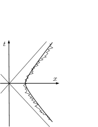
Figure 1: Stochastic trajectories of a uniformly accelerated electron affected by quantum field fluctuations.

This fluctuating motion of the electron changes the acceleration of the electron and may produce additional radiation (the Unruh radiation) to the ordinary Larmor radiation. The rough estimation [2] suggested that the strength of the Unruh radiation is much smaller than the classical one by $10^{-5}$, but the angular dependence becomes quite different. Especially in the direction along the acceleration there is a blind spot for the Larmor radiation while the Unruh radiation is expected to be radiated more spherically. Hence they proposed to detect the Unruh radiation by setting a photon detector in this direction.

The above argument seems intuitively correct, but there are two problems that should be clarified. The first problem is the thermalization time of the fluctuation. The electromagnetic field of laser are not constant but oscillating. One may approximate the electron’s motion around the turning points by a uniform acceleration. This approximation is valid only when the period of the laser is large enough compared to the relaxation time (or thermalization time) of the particle’s fluctuation. Using a stochastic approach, we obtained the relaxation time of the fluctuation and showed that the relaxation time is longer than the period of the laser. In such a case, we must fully analyze the transient dynamics of the fluctuation to calculate the radiation in the laser field.

The second problem is the interference effect. Since the Unruh radiation originates in the interaction with the particle with the quantum fluctuations of the vacuum, we cannot neglect the interference of the Unruh radiation and the vacuum quantum fluctuations. In a simpler model, it has been known that the Unruh radiation is completely canceled by the interference effect. The cancellation was shown for the Unruh detector in both 1+1 and 3+1 dimensions[7, 8]. There was no calculation of the interference effect in the case of the uniformly accelerated charged particle since the calculation needs some technicalities. In the paper [1] we calculated the interference effect for the charged particle in the scalar QED and found that some of the Unruh radiation is canceled by the interference effect, but the cancellation occurs only partially. So we still have a possibility to detect additional radiation from the uniformly accelerated charged particle, but the complete understanding needs more detailed analysis.

In the rest of this report we first briefly review the stochastic model of a uniformly accelerated charged particle and then show how the thermalization of the fluctuation occurs by solving the stochastic equation. Finally we briefly sketch the calculation of the radiation, particularly put emphasis on the interference effect. More details of the calculation of the interference effect and the Unruh radiation are reviewed in another report of the same authors in the proceedings [5].

2 THERMALIZATION

We consider the scalar QED. The model is analyzed in [9] and here we briefly review the settings and the derivation of the stochastic Abraham-Lorentz-Dirac (ALD) equation. The system composes of a relativistic particle $z^{\mu}(\tau)$ and the scalar field $\phi(x)$. The action is given by

$$S[z,\phi,h]= -m\int d\tau\,\sqrt{\dot{z}^{\mu}\dot{z}_{\mu}}+\int d^{4}x\,\frac{1}{2}(\partial_{\mu}\phi)^{2}$$

$$+\int d^{4}x\,j(x;z)\phi(x).$$ (3)

The scalar current $j(x;z)$ is defined as

$$j(x;z)=e\int d\tau\,\sqrt{\dot{z}^{\mu}\dot{z}_{\mu}}\,\delta^{4}(x-z(\tau)),$$ (4)

We choose the parametrization $\tau$ to satisfy $\dot{z}^{2}=1$.

2.1 The Stochastic Equation

The equation of motion of the particle is given by

$$m\ddot{z}^{\mu}=F^{\mu}-\int d^{4}x\frac{\delta j(x;z)}{\delta z_{\mu}(\tau)}\phi(x)$$ (5)

where we have added the external force $F^{\mu}$ so as to accelerate the particle uniformly; $F^{\mu}=ma(\dot{z}^{1},\dot{z}^{0},0,0)$. Then a classical solution of the particle (in the absence of the coupling to $\phi$) is given by

$$z^{\mu}_{0}=(\frac{1}{a}\sinh{a\tau},\frac{1}{a}\cosh{a\tau},0,0).$$ (6)

The equation of motion of the radiation field $\partial^{2}\phi=j$ is solved by using the retarded Green function $G_{R}$ as

$$\phi(x) =\phi_{h}(x)+\phi_{I}(x),$$

$$\phi_{I}(x) =\int d^{4}x^{\prime}G_{R}(x,x^{\prime})j(x^{\prime};z)$$ (7)

where $\phi_{h}$ is the homogeneous solution of the equation of motion and represents the vacuum fluctuation. It is responsible for the particle’s fluctuating motion under a uniform acceleration. Inserting the solution (7) into (5), we have the following stochastic equation for the particle

$$m\ddot{z}^{\mu}(\tau)= F^{\mu}(z(\tau))-e\vec{\omega}^{\mu}$$ (8)

$$\times\left(\phi_{h}(z(\tau))+e\int d\tau^{\prime}\ G_{R}(z(\tau),z(\tau^{\prime}))\right),$$ (9)

where $\vec{\omega}_{\mu}=\dot{z}^{\nu}\dot{z}_{[\nu}\partial_{\mu]}-\ddot{z}_{\mu}$, which comes from the deviation of the current

$$\int d^{4}x\frac{\delta j(x;z)}{\delta z^{\mu}(\tau)}f(x)=e\vec{\omega}_{\mu}f(x)|_{x=z(\tau)}.$$ (10)

The homogeneous part $\phi_{h}(z(\tau))$ of the scalar field describes the Gaussian fluctuation of the vacuum, hence, the first term in the parenthesis of (8) can be interpreted as random noise to the particle’s motion

$$\langle\phi_{h}(x)\phi_{h}(x^{\prime})\rangle=-\frac{1}{4\pi^{2}}\frac{1}{(t-t^{\prime}-i\epsilon)^{2}-r^{2}}.$$ (11)

It is essentially quantum mechanical, but if it is evaluated on a world line of a uniformly accelerated particle $x=z(\tau),x^{\prime}=z(\tau^{\prime})$, it behaves as the ordinary finite temperature noise. The second term in the parenthesis of (8) is a functional of the total history of the particle’s motion $z(\tau^{\prime})$ for $\tau^{\prime}\leq\tau$, but it can be reduced to the so called radiation damping term of a charged particle coupled with radiation field. It is generally nonlocal, but since the Green function damps rapidly as a function of the distance $r$, the term is approximated by local derivative terms. After the mass renormalization, we get the following generalized Langevin equation for the charged particle,

$$m\dot{v}^{\mu}-F^{\mu}-\frac{e^{2}}{12\pi}(v^{\mu}\dot{v}^{2}+\ddot{v}^{\mu})=-e\vec{\omega}^{\mu}\phi_{h}(z)$$ (12)

where $v^{\mu}=\dot{z}^{\mu}$. This equation is an analog of the ALD equation for a charged particle interacting with the electromagnetic field. The dissipation term is induced by the effect of the backreaction of the particle’s radiation to the particle’s motion. Note that, if the noise term is absent, the classical solution (6) with a constant acceleration is still a solution to the equation (12).

2.2 Equipartition Theorem

The stochastic equation (12) is nonlinear and difficult to solve. Here we consider small fluctuations around the classical trajectory induced by the vacuum fluctuation $\phi_{h}$. Especially we consider fluctuations in the transverse directions. First we expand the particle’s motion around the classical trajectory $z^{\mu}_{0}$ as

$$z^{\mu}(\tau)=z^{\mu}_{0}(\tau)+\delta z^{\mu}(\tau).$$ (13)

The particle is accelerated along the $x$ direction. In the following we consider small fluctuation in transverse directions. By expanding the stochastic equation (12), we can obtain a linearized stochastic equation for the transverse velocity fluctuation $\delta v^{i}\equiv\delta\dot{z}^{i}$ as,

$$m\delta\dot{v}^{i}=e\partial_{i}\phi_{h}+\frac{e^{2}}{12\pi}(\delta\ddot{v}^{i}-a^{2}\delta v^{i}).$$ (14)

Performing the Fourier transformation with respect to the trajectory’s parameter $\tau$

$$\delta v^{i}(\tau) =\int\frac{d\omega}{2\pi}\delta\tilde{v}^{i}(\omega)e^{-i\omega\tau},$$ (15)

$$\partial_{i}\phi_{h}(\tau) =\int\frac{d\omega}{2\pi}\partial_{i}\varphi(\omega)e^{-i\omega\tau},$$ (16)

the stochastic equation can be solved as

$$\delta\tilde{v}^{i}(\omega)=eh(\omega)\partial_{i}\varphi(\omega),$$ (17)

where

$$h(\omega)=\frac{1}{-im\omega+\frac{e^{2}(\omega^{2}+a^{2})}{12\pi}}.$$ (18)

The vacuum 2-point function along the classical trajectory can be evaluated from (11) as

$$\langle\partial_{i}\phi_{h}(x)\partial_{j}\phi_{h}(x^{\prime})\rangle|_{x=z(\tau),x^{\prime}=z(\tau^{\prime})}$$

$$=\frac{1}{2\pi^{2}}\frac{\delta_{ij}}{((t-t^{\prime}-i\epsilon)^{2}-r^{2})^{2}}$$

$$=\frac{a^{4}}{32\pi^{2}}\frac{\delta_{ij}}{\sinh^{4}(\frac{a(\tau-\tau^{\prime}-i\epsilon)}{2})}.$$ (19)

It has originated from the quantum fluctuations of the vacuum, but it can be interpreted as finite temperature noise if it is evaluated on the accelerated particle’s trajectory [6]. The Fourier transformation of the symmetrized two point function is evaluated as

$$\langle\partial_{i}\phi(x)\partial_{j}\phi(x^{\prime})\rangle_{S} =\langle\{\partial_{i}\phi(x),\partial_{j}\phi(x^{\prime})\}\rangle/2$$

$$=2\pi\delta(\omega+\omega^{\prime})\delta_{ij}I_{S}(\omega),$$ (20)

where

$$I_{S}(\omega)=\frac{1}{12\pi}\coth\left(\frac{\pi\omega}{a}\right)(\omega^{3}+\omega a^{2}),$$ (21)

which is an even function of $\omega$. The correlator $I_{S}(\omega)$ should be regularized at the UV, which is large $\omega$ or short proper time difference, where quantum field theoretic effects of electron become important. Full QED treatment is necessary there.

For small $\omega$, it is expanded as

$$I_{S}(\omega)=\frac{a}{12\pi^{2}}(a^{2}+O(\omega^{2})).$$ (22)

The expansion corresponds to the derivative expansion

$$\langle\partial_{i}\phi_{h}(x)\partial_{j}\phi_{h}(x^{\prime})\rangle_{S}=\frac{a^{3}}{12\pi^{2}}\delta_{ij}\delta(\tau-\tau^{\prime})+\cdots.$$ (23)

With this expansion, the expectation value of the square of the transverse velocity fluctuation can be evaluated as

$$\langle\delta v^{i}(\tau)\delta v^{j}(\tau^{\prime})\rangle_{S}$$

$$=e^{2}\int\frac{d\omega d\omega^{\prime}}{(2\pi)^{2}}\langle\partial_{i}\varphi(\omega)\partial_{j}\varphi(\omega^{\prime})\rangle_{S}\ h(\omega)h(\omega^{\prime})e^{-i(\omega\tau+\omega^{\prime}\tau^{\prime})}$$

$$\sim e^{2}\delta_{ij}\int\frac{d\omega}{24\pi^{3}}\frac{a^{3}e^{-i\omega(\tau-\tau^{\prime})}}{(m\omega)^{2}+\left(\frac{e^{2}}{12\pi}\right)(\omega^{2}+a^{2})^{2}}.$$ (24)

Here we consider the acceleration of the electron to be at the order 0.1 eV, which is much smaller than the electron mass 0.5 MeV. With the assumption $m\gg a$, one can evaluate the integral and get the following result,

$$\frac{m}{2}\langle\delta v^{i}(\tau)\delta v^{j}(\tau)\rangle=\frac{1}{2}\frac{a\hbar}{2\pi c}\delta_{ij}\left(1+O(a^{2}/m^{2})\right).$$ (25)

Here we have recovered $c$ and $\hbar$. This gives the equipartition relation for the transverse momentum fluctuations in the Unruh temperature $T_{U}=a\hbar/2\pi c$.

2.3 Relaxation Time

The thermalization process of the stochastic equation (14) can be also discussed. For simplicity, we approximate the stochastic equation by dropping the second derivative term. Then it is solved as

$$\delta v^{i}(\tau)= e^{-\Omega_{-}\tau}\delta v^{i}(0)$$

$$+\frac{e}{m}\int_{0}^{\tau}d\tau^{\prime}\ \partial_{i}\phi(z(\tau^{\prime}))e^{-\Omega_{-}(\tau-\tau^{\prime})},$$ (26)

where $\Omega_{-}$ is given by

$$\Omega_{-}=\frac{a^{2}e^{2}}{12\pi m}$$ (27)

The relaxation time is $\tau_{R}=1/\Omega_{-}.$ The velocity square can be also calculated as

$$\langle\delta v^{i}(\tau)\delta v^{j}(\tau)\rangle= e^{-2\Omega_{-}\tau}\delta v^{i}(0)\delta v^{j}(0)$$

$$+\frac{a\delta_{ij}}{2\pi m}(1-e^{-2\Omega_{-}\tau}).$$ (28)

For $\tau\rightarrow\infty$, it approaches the thermalized average (25). The relaxation time in the proper time can be estimated, for the parameter $a=0.1$ eV and $m=0.5$ MeV,

$$\tau_{R}=\frac{12\pi m}{a^{2}e^{2}}\sim 10^{-5}\textrm{sec}.$$ (29)

Let’s compare this relaxation time with the laser frequency. The planned wavelength of the laser at ELI is around $10^{3}$nm and the oscillation period of the laser field is very short; $3\times 10^{-15}$ seconds. So the relaxation time is much longer and the charged particle cannot become thermalized during each oscillation. Hence the assumption of the uniform acceleration in the laser field is not good. Even in such a situation, if the electron is accelerated in the laser field for a long time, an electron may feel an averaged temperature.

The position of the particle in the transverse directions also fluctuates like the ordinary Brownian motion in a heat bath. The mean square of the transverse coordinate $R^{2}(\tau)=\sum_{i=y,z}\langle(z^{i}(\tau)-z^{i}(0))^{2}\rangle$ is calculated as

$$R^{2}(\tau) =2D\left(\tau-\frac{3-4e^{-\Omega_{-}\tau}+e^{-2\Omega_{-}\tau}}{2\Omega_{-}}\right).$$ (30)

with the diffusion constant $D=2T_{U}/(\Omega_{-}m)=12/ae^{2}\sim 8\times 10^{4}\ m^{2}/s.$ In the Ballistic region where $\tau<\tau_{R}$, the mean square becomes $R^{2}(\tau)=2T_{U}\tau^{2}/m$ while in the diffusive region ($\tau>\tau_{R}$), it is proportional to the proper time as $R^{2}(\tau)=2D\tau.$ As the ordinary Brownian motion, the mean square of the particle’s transverse position grows linearly with time. If it becomes possible to accelerate the particle for a sufficiently long period, it may be possible to detect such a Brownian motion in future laser experiments.

3 RADIATION and INTERFERENCE

Now we are ready to calculate the radiation emanated from the uniformly accelerated charged particle. An important point is the interference effect between the quantum fluctuations of the vacuum $\phi_{h}$ and the radiation induced by the fluctuating motion in the transverse directions $\phi_{I}$. First let’s consider the two point function

$$\langle\phi(x)\phi(x^{\prime})\rangle-\langle\phi_{h}(x)\phi_{h}(x^{\prime})\rangle$$ (31)

$$=\langle\phi_{I}(x)\phi_{h}(x^{\prime})\rangle+\langle\phi_{h}(x)\phi_{I}(x^{\prime})\rangle+\langle\phi_{I}(x)\phi_{I}(x^{\prime})\rangle.$$

The Unruh radiation estimated in [2] corresponds to calculating the 2-point correlation function of the inhomogeneous terms $\langle\phi_{I}\phi_{I}\rangle$. (The same term also contains the Larmor radiation.) However, this is not the end of the story. As it has been discussed in [7], the interference terms $\langle\phi_{I}\phi_{h}\rangle+\langle\phi_{h}\phi_{I}\rangle$ may possibly cancel the Unruh radiation in $\langle\phi_{I}\phi_{I}\rangle$ after the thermalization occurs. This is shown for an internal detector, but it is not obvious whether the same cancellation occurs for the case of a charged particle we are considering.

The energy-momentum tensor of the radiation field can be obtained from the 2-point function

$$\langle T_{\mu\nu}\rangle=\langle:\partial_{\mu}\phi\partial_{\nu}\phi-\frac{1}{2}g_{\mu\nu}\partial^{\alpha}\phi\partial_{\alpha}\phi:\rangle_{S}.$$ (32)

It is written as a sum of the classical part and the fluctuating part $T_{\mu\nu}=T_{cl,\mu\nu}+T_{fluc,\mu\nu}$. The classical part corresponds to the Larmor radiation while the fluctuating part contains both of the Unruh radiation and the interference terms.

In [1] we calculated the 2-point function including the interference term, and obtained the energy-momentum tensor. The result we have obtained is summarized in [5] in this proceedings. Some terms are partially canceled but not all. Hence, it seems that the uniformly accelerated charged particle emits additional radiation besides the Larmor radiation. The remaining terms after the partial cancellation are proportional to $a^{3}$ and suppressed compared to the Larmor radiation. It has a different angular distribution, but the additional radiation also vanishes in the forward direction.

4 SUMMARY

We have systematically studied the thermalization of a uniformly accelerated charged particle in the scalar QED using the stochastic method, and calculated the radiation by the particle. Two main messages of are

1. ”Long relaxation time compared to the laser period”

2. ”Importance of the interference”

The fluctuation of the particle doesn’t become thermalized during the period of the laser, and we need to study transient dynamics to obtain the radiation from an electron accelerated in the oscillating laser field. The issue of the interference terms are more subtle. Since the particle fluctuation originates in the quantum vacuum fluctuation of the radiation field, it can be by no means neglected. Our result shows that the interference term partially cancels the Unruh radiation, but some of them survives. The remaining Unruh radiation is smaller compared to the Larmor radiation by a factor $a$ (acceleration) and has a different angular distribution. In this sense, it is qualitatively consistent with the proposal [2]. But as we briefly review in [5], the additional radiation also vanishes in the forward direction. and it seems difficult to detect such additional radiation experimentally so far as the transverse fluctuation is concerned. Please beware that the longitudinal fluctuations which we have not calculated yet (because of technical difficulties related to a choice of gauge) may change the situation.

References

- [1] S. Iso, Y. Yamamoto and S. Zhang, arXiv:1011.4191 [hep-th].
- [2] P. Chen and T. Tajima, Phys. Rev. Lett. 83 (1999) 256.
- [3] P.G. Thirolf, et.al. Eur. Phys. J. D 55, 379-389 (2009).
- [4] http://www.extreme-light-infrastructure.eu/
- [5] S. Iso, Y. Yamamoto and S. Zhang, in the same proceedings, “Unruh radiation and Interference effect”
- [6] W. G. Unruh, Phys. Rev. D 14, 870 (1976).
- [7] D. J. Raine, D. W. Sciama and P. G. Grove, Proc. R. Soc. Lond. A (1991) 435, 205-215
- [8] A. Raval, B. L. Hu, J. Anglin, Phys. Rev. D 53 (1996) 7003.
- [9] P. R. Johnson and B. L. Hu, arXiv:quant-ph/0012137. Phys. Rev. D 65 (2002) 065015 [arXiv:quant-ph/0101001].