Conductance of a helical edge liquid coupled to a magnetic impurity

Abstract

Transport in an ideal two-dimensional quantum spin Hall device is dominated by the counterpropagating edge states of electrons with opposite spins, giving the universal value of the conductance, $2e^{2}/h$. We study the effect on the conductance of a magnetic impurity, which can backscatter an electron from one edge state to the other. In the case of isotropic Kondo exchange we find that the correction to the electrical conductance caused by such an impurity vanishes in the dc limit, while the thermal conductance does acquire a finite correction due to the spin-flip backscattering.

Topological insulators have been actively studied in the last few years review . In these systems the bulk of the sample is insulating, with gapless electronic excitations allowed only at the boundary. One example of this phenomenon, the quantum Hall effect, is realized in two-dimensional electron systems placed in a strong magnetic field perpendicular to the sample. Another example is the so-called quantum spin Hall (QSH) effect, recently observed in HgTe quantum wells konig . It is present in time-reversal invariant two-dimensional systems, and can be viewed as two coexisting quantum Hall states for opposite spin subsystems. Although no external magnetic field is present, an effective field is generated via spin-orbit coupling. The sign of the field is opposite for spin-$\uparrow$ and spin-$\downarrow$ electrons, resulting in two edge states propagating in opposite directions.

In the absence of defects, the conductance measured between two contacts attached to the edges of a quantum spin Hall device is $2e^{2}/h$. (Here $e$ is the electron charge and $h$ is the Planck’s constant.) This can be understood, e.g., as twice the conductance of a standard quantum Hall structure, as the number of the edge states is doubled. The presence of two counterpropagating edge states also allows for the possibility of backscattering of electrons, which would reduce the conductance. However, such backscattering processes are strongly restricted by the time-reversal symmetry wu ; xu . In particular, an impurity without internal degrees of freedom cannot backscatter a single electron at the edge, though backscattering of two electrons is allowed. Another allowed process is backscattering of a single electron by a magnetic impurity.

The effect of a magnetic impurity on the conductance of a QSH device was discussed recently by Maciejko et al. maciejko . They argued that at high temperature the backscattering by magnetic impurity gives a small negative correction to the conductance. As the temperature $T$ is lowered, the Kondo effect enhances the backscattering and the correction grows. The trend then reverses at $T$ of the order of the Kondo temperature, and at $T=0$ the quantized conductance $2e^{2}/h$ is restored. In this Letter we study the correction $\delta G$ to the conductance as a function of frequency $\omega$, focusing on the case of isotropic Kondo exchange and neglecting the two-particle backscattering. Our results for $\delta G(\omega)$ agree with the predictions by Maciejko et al. maciejko when $\omega$ exceeds a certain relaxation rate, whereas in the dc limit $\omega\to 0$ we find $\delta G=0$.

Following Refs. wu ; xu ; maciejko , we combine the two edge states into a single nonchiral Tomonaga-Luttinger liquid and write its Hamiltonian in the standard bosonized form giamarchi

$$H_{0}=\frac{\hbar v}{2\pi}\int dx[K(\partial_{x}\theta)^{2}+K^{-1}(\partial_{x}\phi)^{2}].$$ (1)

Here $v$ is the velocity of the edge states, and parameter $K$ accounts for the interactions between the electrons at the edge, with the repulsive interactions corresponding to $K<1$. The bosonic fields $\theta(x)$ and $\phi(x)$ satisfy the commutation relations $[\phi(x),\partial_{y}\theta(y)]=i\pi\delta(x-y)$. For simplicity, we limit ourselves to the case of spin-$\frac{1}{2}$ impurity, and write the Kondo coupling to the edge states using the standard boson representation of the electron operators $\psi_{\uparrow,\downarrow}=(2\pi\alpha)^{-1/2}e^{-i(\theta\pm\phi)}$, where $\alpha$ is the short distance cutoff and we assigned spins up and down to the right- and left-moving electrons, respectively. We allow for the possibility of anisotropic coupling and write the spin-flip term as

$$H_{\perp}=\frac{J_{\perp}}{2\pi\alpha}[e^{2i\phi(0)}S^{+}+e^{-2i\phi(0)}S^{-}],$$ (2)

where $S^{\pm}=S^{x}\pm iS^{y}$ and $S^{i}$ are spin operators. In addition, the $z$ component of the impurity spin is coupled to the Tomonaga-Luttinger liquid via

$$H_{z}=-\frac{J_{z}}{\pi}\partial_{x}\theta(0)S^{z}.$$ (3)

For convenience, our Hamiltonian allows for uniaxial exchange anisotropy, which disappears at $J_{z}=J_{\perp}$. Up to a minor difference in notation, the Hamiltonian (1)–(3) coincides with the expression used in Refs. wu ; maciejko .

To discuss the conductance of the device, one has to add to the Hamiltonian a term accounting for the applied bias. The most straightforward approach is to assign different chemical potentials $\pm eV/2$ to the right- and left-moving electrons. Such a perturbation takes the form

$$H_{V}=-\frac{eV}{2\pi}\int dx\,\partial_{x}\theta.$$ (4)

One should note that assigning the same chemical potential to all the electrons moving in the same direction is an approximation. It assumes that the backscattering by impurity is weak, $\delta G\ll e^{2}/h$, and that $\omega\ll v/L$, where $L$ is the distance between the source and drain contacts.

The operator (4) commutes with $H_{0}$ and $H_{z}$, and its only effect is to change the energy by $\pm eV$ each time an electron is backscattered and the impurity spin is flipped by $H_{\perp}$. The same effect is achieved by assigning different energy values to the up and down components of the impurity spin, i.e., by replacing (4) with an effective magnetic field term

$$H_{V}=-eVS^{z}.$$ (5)

This replacement can be more formally justified by noticing that the difference of the operators (4) and (5) commutes with the Hamiltonian.

To simplify the subsequent calculations it is convenient to rescale the bosonic fields $\{\phi,\theta\}\to\{\sqrt{K}\phi,\theta/\sqrt{K}\}$ and then perform the unitary transformation $U=e^{i\lambda\phi(0)S^{z}}$. For $\lambda=J_{z}/\pi\hbar v\sqrt{K}$ the additional term arising from the transformation of $H_{0}$ cancels the coupling (3) of the $z$ components of spins, resulting in the Hamiltonian

$${\tilde{H}}_{0} = \frac{\hbar v}{2\pi}\int dx[(\partial_{x}\theta)^{2}+(\partial_{x}\phi)^{2}],$$ (6)

$${\tilde{H}}_{\perp} = \frac{J_{\perp}}{2\pi\alpha}[e^{i2\sqrt{\tilde{K}}\phi(0)}S^{+}+e^{-i2\sqrt{\tilde{K}}\phi(0)}S^{-}],$$ (7)

with the bias contribution (5) retaining its form. The advantage of this procedure is that the effect of electron-electron interactions and coupling of $z$ components of spins are now accounted for by a single parameter $\tilde{K}=K(1-J_{z}/2\pi\hbar vK)^{2}$.

Our first goal is to evaluate the correction $\delta G(\omega)$ to the conductance of the system due to the backscattering of electrons by the impurity. Since backscattering of a right-moving electron is always accompanied by the impurity spin flip from $\downarrow$ to $\uparrow$, the correction to the current can be computed as the time derivative of $S^{z}$, i.e., $\delta I=-e\partial_{t}S^{z}$. With the Hamiltonian in the form (5)–(7) one immediately obtains

$$\delta I=\frac{ie}{\hbar}\,\frac{J_{\perp}}{2\pi\alpha}[e^{i2\sqrt{\tilde{K}}\phi(0)}S^{+}-e^{-i2\sqrt{\tilde{K}}\phi(0)}S^{-}].$$ (8)

In the linear response theory the conductance can be found using the Kubo formula, which expresses $\delta G(\omega)$ in terms of the current-current correlator. The latter cannot be found exactly for arbitrary values of the parameters $\tilde{K}$ and $J_{\perp}$. Assuming weak coupling (7), one can evaluate $\delta G$ to the lowest order in $J_{\perp}$, which results in the following expression:

$$\delta G(\omega) = -\frac{2e^{2}}{\hbar^{3}}\left(\frac{J_{\perp}}{2\pi\alpha}\right)^{2}\left(\frac{\pi T}{D}\right)^{2\tilde{K}}\sin(\pi\tilde{K})$$ (9)

$$\times\frac{1}{i\omega}\int_{0}^{\infty}\frac{(e^{i\omega t}-1)dt}{[\sinh(\pi Tt/\hbar)]^{2\tilde{K}}}.$$

Here we have introduced the bandwidth $D=\hbar v/\alpha$.

In the most interesting regime of low frequencies, $\hbar\omega\ll T$, the conductance is

$$\delta G=-\frac{e^{2}\gamma_{0}}{2T},$$ (10)

where $\gamma_{0}$, defined as

$$\gamma_{0}=J_{\perp}^{2}\Upsilon,\quad\Upsilon=\frac{[\Gamma(\tilde{K})]^{2}}{(2\pi\hbar)^{2}\alpha v\Gamma(2\tilde{K})}\left(\frac{2\pi T}{D}\right)^{2\tilde{K}-1},$$ (11)

has the meaning of the rate of spin-flip processes at $V=0$. The same result was obtained by a similar method by Maciejko et al. maciejko . It is important to realize that the derivation relied on the perturbation theory in $J_{\perp}$. Let us now show that at low frequencies $\omega\ll\gamma_{0}\propto J_{\perp}^{2}$ the conductance deviates from (10).

To this end we consider the dynamics of the impurity spin at finite temperature and weak spin-flip coupling, $\gamma_{0}\ll T/\hbar$. In this case, the spin remains in the $\uparrow$ or $\downarrow$ state for a long time. The rates of spin-flip events are easily computed and take the form

$$\gamma_{\pm}=\gamma_{0}\left(1\pm\frac{eV}{2T}\right)$$ (12)

for small voltage $eV\ll T$, where $\gamma_{+}$ and $\gamma_{-}$ are the rates of up-flip and down-flip, respectively.

At any given moment the impurity spin can be in either $\uparrow$ or $\downarrow$ state, and its behavior is described by the probabilities $P_{\uparrow}$ and $P_{\downarrow}$. Their time dependence can be found from a simple rate equation

$$\partial_{t}P_{\uparrow}=\gamma_{+}P_{\downarrow}-\gamma_{-}P_{\uparrow}$$ (13)

and the condition $P_{\uparrow}+P_{\downarrow}=1$. Each spin flip is accompanied by backscattering of a single electron. The resulting correction to the electric current is $\delta I=-e\partial_{t}P_{\uparrow}$. To find the linear conductance one substitutes the rates in the form (12) with $V=V_{0}e^{-i\omega t}$ into (13), and calculates $\delta G=\delta I/(V_{0}e^{-i\omega t})$. This procedure yields

$$\delta G(\omega)=-\frac{e^{2}\gamma_{0}}{2T}\,\frac{\omega}{\omega+2i\gamma_{0}}.$$ (14)

The rate equation approach is applicable only at relatively low frequencies, $\hbar\omega\ll T$. In a broad frequency range $\gamma_{0}\ll\omega\ll T/\hbar$ expression (14) recovers the perturbative result (10).

The results (10) and (14) differ dramatically in the dc limit, $\omega\to 0$, where the correction (14) vanishes. This is easily understood if one notices that every time an electron is backscattered to the left (right) the impurity spin is flipped up (down). Thus, the backscattering current changes its direction with every spin flip, and in the dc limit the correction to the conductance vanishes. This argument also applies at $T\lesssim\hbar\gamma_{0}$, when the rate equation approach is no longer applicable.

To illustrate this point, we consider a special case $\tilde{K}=\frac{1}{2}$, in which the dimension of the operator $\exp[i2\sqrt{\tilde{K}}\phi(0)]$ in the definition of the spin-flip operator (7) is $\frac{1}{2}$, maciejko . This case corresponds to the well-understood Toulouse limit of the Kondo model, in which the Hamiltonian can be reduced to that of a system of noninteracting chiral spinless fermions $\Psi(x)$ coupled to a discrete level:

$$H = -i\hbar v\int\Psi^{\dagger}(x)\partial_{x}\Psi(x)dx-eVd^{\dagger}d$$ (15)

$$+\frac{J_{\perp}}{\sqrt{2\pi\alpha}}[d^{\dagger}\Psi(0)+\Psi^{\dagger}(0)d].$$

Here $d$ is the annihilation operator of a fermion at the discrete level which models the impurity spin, $S^{z}=d^{\dagger}d-\frac{1}{2}$. The model (15) is easily solved exactly, resulting in

$$\delta G(\omega)=-i\iint\frac{\omega[n(\xi_{2})-n(\xi_{1})]}{\hbar\omega-\xi_{1}+\xi_{2}+i\delta}\frac{(e\Gamma/\pi)^{2}d\xi_{1}d\xi_{2}}{(\xi_{1}^{2}+\Gamma^{2})(\xi_{2}^{2}+\Gamma^{2})}.$$ (16)

Here the level width $\Gamma=J_{\perp}^{2}/4\pi\hbar\alpha v$ coincides with $\hbar\gamma_{0}$ for $\tilde{K}=1/2$, Eq. (11), and $n(\xi)=1/(e^{\xi/T}+1)$ is the occupation probability of a fermion state with energy $\xi$ measured from the Fermi level.

In the high-temperature limit $T\gg\Gamma$ one can expand the difference of the Fermi functions in the numerator to linear order in $\xi_{2}-\xi_{1}$. This approximation recovers our earlier result (14) with $\gamma_{0}=\Gamma/\hbar$. Importantly, the Toulouse limit expression (16) for $\delta G(\omega)$ does not rely on the rate equation approach and is therefore valid for any temperature. It is easy to see that in the dc limit the expression (16) vanishes for any $T$. The dependence $\delta G(\omega)$ at various temperatures is shown in Fig. 1.

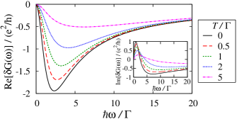
Figure 1: (color online) Real part and imaginary part of $\delta G(\omega)$ for several temperatures $T/\Gamma$.

In the absence of corrections to the quantized dc conductance of the system, it is interesting to explore whether other transport properties are affected by coupling to the impurity. One such property is the thermal conductance $\mathcal{K}$. Let us assume that the left- and right-moving electrons originate in the leads with different temperatures, $T$ and $T+\Delta T$, respectively. Spin-flip scattering by the impurity gives rise to two kinds of electron scattering processes. The electrons are either scattered from the warmer right-moving system to a colder left-moving one, or in the opposite direction. These two types of processes change the charge of the right-moving system by $e$ and $-e$, respectively, resulting in no correction to the time-averaged electric current. On the other hand, each scattering process transfers heat in the same direction: from the warm right-moving system to the cold left-moving one. As a result, one expects to find a finite negative correction $\delta\mathcal{K}$ to the thermal conductance of the system.

To evaluate $\delta\mathcal{K}$, we identify the operator of the difference of energies in the right- and left-moving branches $\delta\tilde{H}=(\tilde{H}_{0}^{R}-\tilde{H}_{0}^{L})/2$. The energy densities of the two subsystems are given by $\hbar v[\partial_{x}(\phi\mp\theta)]^{2}/4\pi$, leading to

$$\delta\tilde{H}=-\frac{\hbar v}{2\pi}\int\partial_{x}\phi\,\partial_{x}\theta dx.$$ (17)

The operator $\delta J_{E}$ of the energy current transferred between the right- and left-moving branches is then found as the time derivative of (17), resulting in

$$\delta J_{E}=-\frac{\hbar v\sqrt{\tilde{K}}}{e}\,\partial_{x}\phi(0)\,\delta I,$$ (18)

where $\delta I$ is the electric current operator in Eq. (8).

It is worth noting that the operators $\partial_{x}\phi(0)$ and $\delta I$ act in separate subspaces of odd and even $\phi(x)$. In particular, the dynamics of $\partial_{x}\phi(0)$ is not affected by the coupling (7) to the impurity. A similar observation was made by Kane and Fisher kanefisher in the study of thermal transport of a Luttinger liquid through a tunneling barrier. They used the factorization of the energy current operator similar to Eq. (18) to obtain a relation between the thermal and electrical conductances of the system. Repeating their procedure for our Hamiltonian, we obtain the expression

$$\delta{\mathcal{K}}=\frac{\hbar^{3}\tilde{K}}{8e^{2}T^{2}}\int_{-\infty}^{\infty}\frac{\omega^{2}{\rm Re\,}\delta G(\omega)}{\sinh^{2}(\hbar\omega/2T)}d\omega,$$ (19)

fully analogous to Eq. (19) of Ref. kanefisher .

The relation (19) shows that thermal conductance is determined by the electrical conductance at frequencies $\omega\sim T/\hbar$. As a result, the fact that $\delta G$ vanishes at $\omega\to 0$ does not mean that there will be no correction to $\mathcal{K}$. For instance, in the lowest order in spin-flip scattering (7), one can find $\delta\mathcal{K}$ by substituting into Eq. (19) $\delta G(\omega)$ in the form (9). This procedure yields

$$\delta\mathcal{K}=-\frac{\pi^{2}}{2}\,\frac{\tilde{K}^{2}}{2\tilde{K}+1}\,\gamma_{0}.$$ (20)

Within the applicability of the perturbation theory, $\hbar\gamma_{0}\ll T$, this correction is small compared to the nominal value ${\mathcal{K}}_{0}=\pi^{2}T/3h$ of the thermal conductance of a Kramers’ pair of edge states.

At $\hbar\gamma_{0}\sim T$ the perturbative approach is not applicable, but an exact solution is possible in the Toulouse limit, $\tilde{K}=1/2$. Substituting the conductance (16) into Eq. (19) we obtain

$$\delta\mathcal{K}=\frac{\Gamma^{2}}{8hT^{2}}\iint\frac{(\xi_{2}-\xi_{1})^{3}[n(\xi_{2})-n(\xi_{1})]d\xi_{1}d\xi_{2}}{(\xi_{1}^{2}+\Gamma^{2})(\xi_{2}^{2}+\Gamma^{2})\sinh^{2}[(\xi_{2}-\xi_{1})/2T]}.$$ (21)

At high temperatures ($T\gg\Gamma$), $\delta\mathcal{K}=-\pi^{2}\Gamma/16\hbar$, in agreement with the perturbative result (20). On the other hand, the fact that ${\rm Re}\,\delta G(\omega)\propto\omega^{2}$ at $\omega\to 0$ means that the correction $\delta\mathcal{K}$ in Eq. (19) is suppressed as $T^{3}$ at low temperatures, $T\ll\Gamma$. Indeed, from Eq. (21) one finds $\delta\mathcal{K}=-2\pi^{3}T^{3}/15\hbar\Gamma^{2}$ in this regime.

The suppression of $\delta\mathcal{K}$ in both the low- and high-temperature limits results in nonmonotonic behavior of the normalized thermal conductance $\mathcal{K}/\mathcal{K}_{0}$ as a function of temperature, Fig. 2. Such nonmonotonic behavior was predicted for the electrical conductance by Maciejko et al. maciejko , based on the well-known nonmonotonic temperature dependence of the spin-flip scattering in the Kondo problem. Although our theory predicts quantized dc conductance $2e^{2}/h$ at any temperature, the nonmonotonic temperature dependence is recovered for thermal transport.

Figure 2: Nonmonotonic temperature dependence of the thermal conductance $\mathcal{K}=\mathcal{K}_{0}+\delta\mathcal{K}$ in the Toulouse limit, Eq. (21).

At $T\lesssim\gamma_{0}$ and $\omega\sim\gamma_{0}$ our correction to the electrical conductance can take rather large values $|\delta G(\omega)|\sim e^{2}/h$, see, e.g., Fig. 1. We do not believe the correction $\delta G(\omega)$ has a clear physical meaning in this regime, as the conditions for the applicability of the model (4) are violated. This caveat, however, does not apply to our main conclusion, namely vanishing $\delta G$ at $\omega\to 0$. Similarly, the behavior of the thermal conductance shown in Fig. 2 is only qualitatively correct at $T\sim\Gamma$, where the relative correction $\delta\mathcal{K}/\mathcal{K}_{0}$ is of order unity.

The main feature of our work, the absence of correction to the dc conductance due to Kondo scattering, is caused by the symmetry of the Hamiltonian (1)–(3) that preserves the $z$ component of the total spin of the system. Our model is justified if the magnetic impurity is approximated as a single-orbital Anderson impurity, in which case the Kondo exchange is isotropic, $J{\boldsymbol{\sigma}}\cdot{\boldsymbol{S}}$, even in the presence of spin-orbit coupling shekhtman . Anisotropic corrections may appear in the case of multiple orbitals anisotropicexchange . Exchange anisotropy can break the conservation of the $z$ component of the total spin and result in nonvanishing correction to the dc conductance. In the simplest model of anisotropic exchange $J_{i}\sigma^{i}S^{i}$ with $J_{x}\neq J_{y}$ the correction to the dc conductance above the Kondo temperature is easily found from the rate equation approach,

$$\delta G=-\frac{e^{2}\Upsilon}{4T}\,\frac{(J_{x}^{2}-J_{y}^{2})^{2}}{J_{x}^{2}+J_{y}^{2}},$$ (22)

with $\Upsilon$ defined by Eq. (11). At $T$ below the Kondo temperature the impurity spin is screened, and the effect of exchange anisotropy is reduced to that of an impurity-induced two-electron backscattering. The effect of these processes on conductance was studied in Ref. maciejko and found to be suppressed at $T\to 0$ as $T^{2(4K-1)}$.

Another limitation of our model is the assumption that all electrons moving in the same direction have the same spin. Kramers degeneracy guarantees that electrons with momenta $\pm p$ have opposite spins, and we defined the $z$ axis as the direction of the spin of the right mover at the Fermi level, which is determined by the specific form of spin-orbit coupling. Transport is controlled by electrons with momenta $|p\pm p_{F}|\sim T/v$, whose spins may deviate slightly from the $z$ direction defined at $p=p_{F}$. This deviation may result in a correction to the dc conductance vanishing at low temperatures as a power of $T/D$.

The authors are grateful to B. I. Halperin and S. C. Zhang for helpful discussions. A.F. and K.A.M. are grateful to the Aspen Center for Physics, where part of the work was performed, for hospitality. This work was supported by a Grant-in-Aid for Scientific Research from JSPS, Japan (No. 21540332) and by the U.S. DOE, Office of Science, under Contract No. DE-AC02-06CH11357.

References

- (1) For reviews see, e.g., M. Z. Hasan and C. L. Kane, Rev. Mod. Phys. 82, 3045 (2010); X.-L. Qi and S.-C. Zhang, arXiv:1008.2026 [Rev. Mod. Phys. (to be published)].
- (2) M. König et al., Science 318, 766 (2007).
- (3) C. Wu, B. A. Bernevig, and S. C. Zhang, Phys. Rev. Lett. 96, 106401 (2006).
- (4) C. Xu and J. E. Moore, Phys. Rev. B 73, 045322 (2006).
- (5) J. Maciejko et al., Phys. Rev. Lett. 102, 256803 (2009).
- (6) T. Giamarchi, Quantum Physics in One Dimension, (Clarendon Press, Oxford, 2004).
- (7) C. L. Kane and M. P. A. Fisher, Phys. Rev. Lett. 76, 3192 (1996).
- (8) L. Shekhtman, O. Entin-Wohlman, and A. Aharony, Phys. Rev. Lett. 69, 836 (1992).
- (9) S. Gangadharaiah, J. Sun, and O. A. Starykh, Phys. Rev. Lett. 100, 156402 (2008); G. Jackeli and G. Khaliullin, Phys. Rev. Lett. 102, 017205 (2009).