Velocity-space substructure from nearby RAVE and SDSS stars

Abstract

We extract a sample of disc stars within 200 pc of the Sun from the RAVE and SDSS surveys. Distances are estimated photometrically and proper motions are from ground-based data. We show that the velocity-space substructure first revealed in the Geneva-Copenhagen sample is also present in this completely independent sample. We also evaluate action-angle variables for these stars and show that the Hyades stream stars in these data are again characteristic of having been scattered at a Lindblad resonance. Unfortunately, analysis of such local samples can determine neither whether it is an inner or an outer Lindblad resonance, nor the multiplicity of the pattern.

1 The Local Distribution of Stellar Velocities

Analysis of the Hipparcos data by Dehnen (1998) revealed that the stellar velocity distribution in the solar neighbourhood manifested significant substructure. The heroic Geneva-Copenhagen Survey (hereafter GCS Nordström et al., 2004; Holmberg et al., 2009) followed up with radial velocity measurements of 14 139 nearby F and G dwarf stars, which confirmed and strengthened Dehnen’s conclusion.

The Geneva-Copenhagen survey was constructed so as to avoid most of the selection biases that went into the full Hipparcos sample. Aside from a concentration of 112 stars in the Hyades cluster, the distribution of sample stars over the sky is remarkably uniform, with a slightly higher density in the declination range south of $\delta=-26^{\circ}$. The large majority of stars are within 200 pc of the Sun and the sample within 40 pc is believed to be nearly complete.

The Cartesian heliocentric velocity components of stars near the Sun in Galactic coordinates are $U$, $V$ and $W$, with $U$ being directed towards the Galactic centre, $V$ being in the direction of Galactic rotation, and $W$ towards the north Galactic pole. The velocity substructure in the GCS is particularly evident in the $U-V$ plane, where the distribution is broken into a number of substantial streams, with no underlying smooth component. Numerous studies (Famaey et al., 2007; Bensby et al., 2007; Bovy & Hogg, 2010; Pompéia et al., 2011) have shown that the streams are both too substantial and chemically inhomogeneous to be dissolved star clusters (e.g. Eggen, 1996).

Dynamical evolution is the most likely source of the features, which have been modelled extensively. De Simone et al. (2004) suggest that the entire velocity distribution arises from a succession of transient spiral perturbations, while Helmi et al. (2006) attribute some substructure to minor accretion events. Individual features have been modelled as responses to the bar and/or various assumed spiral perturbations within the disc (Dehnen, 2000; Quillen, 2003; Quillen & Minchev, 2005; Chakrabarty, 2007; Antoja et al., 2009; Minchev et al., 2010). The analysis of Quillen & Minchev (2005), which was extended by Pompéia et al. (2011), identified the inner ultra-harmonic resonance of an assumed 2-arm spiral as a possible cause of both the Hyades and Sirius streams.

By contrast, Sellwood (2010, hereafter Paper I) presented an analysis that did not need to assume a form for the perturbation. Using action-angle coordinates, he showed that the stars of the Hyades stream were both concentrated along a resonance line in action space and grouped in a combination of angle coordinates (possibly) indicative of a recent inner Lindblad resonance (hereafter ILR). McMillan (2011) has confirmed most of his analysis, and concurs that a Lindblad resonance is responsible but, unfortunately, was able to show that subtle selection effects in such local data imply that the distribution could also be consistent with trapping in an outer Lindblad resonance (OLR). We discuss selection effects and McMillan’s analysis in the Appendix.

While the GCS sample offered compelling evidence for a Lindblad resonance, it is desirable to attempt to confirm the result from other independent surveys. The Radial Velocity Experiment (RAVE, Steinmetz et al., 2006), a large spectroscopic survey of stars in the southern sky, plans to measure the heliocentric radial velocities and stellar parameters for about a million stars in the apparent magnitude range $9<m_{I}<12$; the first $21\,121$ were made available in the second data release (Zwitter et al., 2008). The typical uncertainty in the radial velocity is $<2\;$km s^-1, but the distance to most stars has to be judged photometrically and most proper motions are from ground-based data. Thus the three phase space coordinates for each star are of much lower quality than are those in the Geneva-Copenhagen survey, although this weakness will, when the survey is complete, be compensated by a much larger sample size. The huge northern Sloan Digital Sky Survey (SDSS, York et al., 2000) and Segue2 (Yanny et al., 2009) surveys are complete, but sample fainter stars (the magnitude range for Segue2 was $14.0<g<20.3$) that are therefore generally more distant than are the RAVE stars. The recently-released M-dwarf sample of SDSS stars (West et al., 2011) substantially increases the number of stars with estimated distances and kinematics within the neighbourhood of the Sun.

2 Sample selection

2.1 RAVE stars

We have downloaded the on-line table of the second data release from the RAVE website and selected a subset of stars for analysis. We estimate distances to these stars by fitting to the Yonsei-Yale isochrones (Demarque et al., 2004) using a method related to that described by Breddels et al. (2010). We adopt many of their selection criteria: we require the spectral signal-to-noise parameter $>20$ with a blank spectral warning flag field; the parameters [M/H], log($g$), and $T_{\rm eff}$ to be determined; and the stars to have J & K_s magnitudes from two-micron all sky survey (2MASS S, 2006) with no warning flags about the identification of the star or the 2MASS photometry. Unlike those authors, however, we have kept stars with $b<25\degr$ on the grounds that extinction for the nearby stars that interest us will not be large enough in the near IR to severely bias our distance estimates. As we wish to select nearby main-sequence stars that are members of the disc population, we also eliminate stars with log$(g)<4$, $T_{\rm eff}>10^{4}\;$K, and with $|v_{r}|>80\;$km s^-1.

Figure 1: Histograms of distances and $U$-velocity uncertainties for the selected sample of 5145 RAVE stars.

We estimate the absolute J magnitude of each selected star by matching the estimated [Fe/H], log($g$), $T_{\rm eff}$, and J-K_s colour to values in the isochrone tables for stars of all ages and all values of [$\alpha$/Fe], rejecting a few more stars for which the best match $\chi^{2}>6$. We consider the closest match in the tables to the given input parameters to yield the best estimate of the absolute magnitude from which we estimate a photometric distance using the apparent J-band magnitude. Our resulting sample contains $7\,384$ stars. We save the values of [Fe/H], log($g$), $T_{\rm eff}$, and J-K_s colour of the closest matching model star in the isochrone table; Monte-Carlo variation of the stellar parameters about this saved set of values suggests that distances have a relative precision of 30% – 50%, with some larger uncertainties.

We use the proper motions in equatorial coordinates tabulated in RAVE, mostly from Tycho-2 (Høg et al., 2000), which we then combine with the radial velocity and position to determine the heliocentric velocity in Galactic components $U,\;V\;\&\;W$ (Johnson & Soderblom, 1987; Piatek et al., 2002). We estimate uncertainties in these velocities from 5000 Monte Carlo re-selections of all the stellar parameters that affect the distance estimate, adopting $\sigma({\rm J})=0.03\;$mag, $\sigma({\rm J-K}_{s})=0.042\;$mag, $\sigma(T_{\rm eff})=300\;$K, $\sigma(\log\,g)=0.3\;$dex, and $\sigma([{\rm Fe/H}])=0.25\;$dex (Breddels et al., 2010), as well as the tabulated radial velocity and proper motion uncertainties.

In order to select nearby thin disc stars, we further restrict the sample to stars whose best estimate of the distance is within $500\;$pc and retain only those having an energy of vertical motion about the Galactic mid-plane, $E_{z}=0.5(z^{2}\nu^{2}+W^{2})<392\;$(km s${}^{-1})^{2}$, with the vertical frequency $\nu=0.07\;$km s^-1 pc^-1 (Binney & Tremaine, 2008), giving them a maximum vertical excursion of $\pm 400\;$pc. This latter restriction rejects most thick disk and halo stars, as well as a few thin disc stars.

Fig. 1 shows histograms of distances and of velocity uncertainties for the $5,145$ remaining stars. The mode of the distance distribution is 200 pc from the Sun. The estimated uncertainties in $U$ are generally $<10\;$km s^-1, with a tail up to values four times larger.

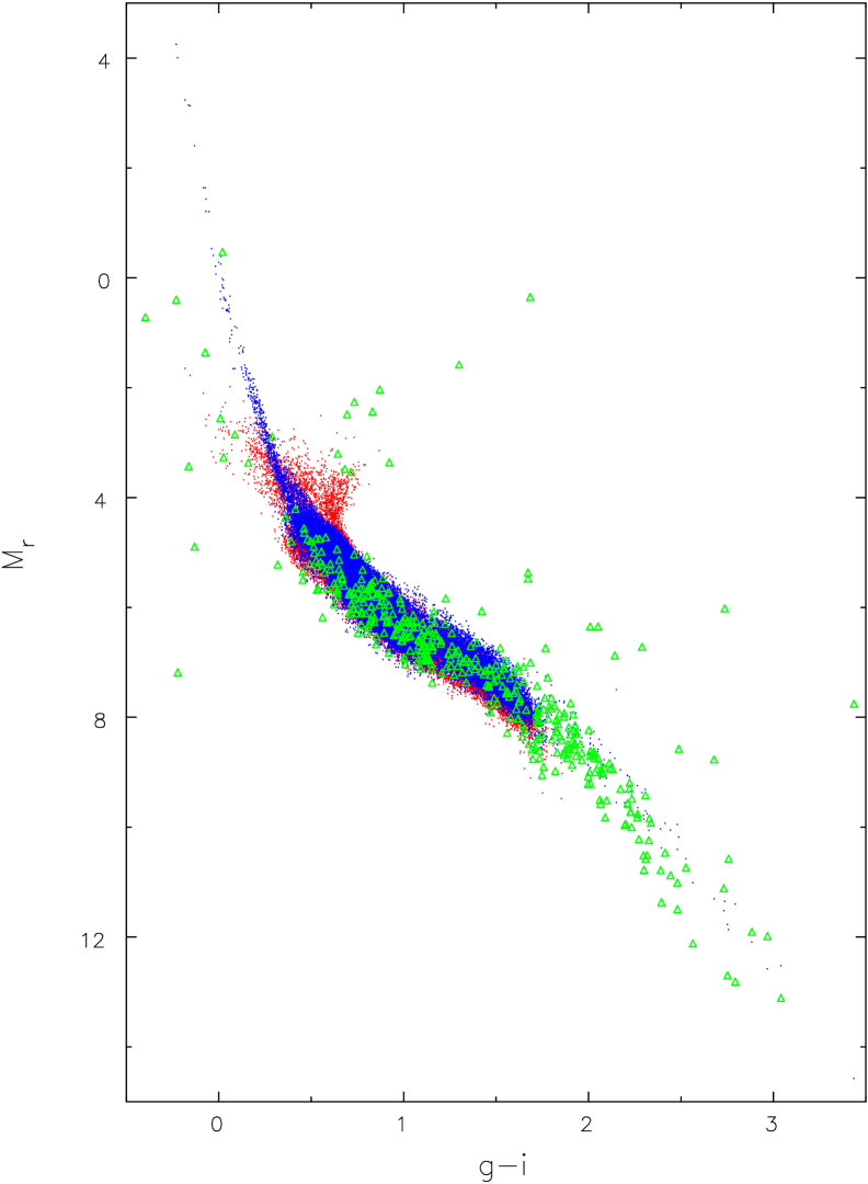
Figure 2: Blue points show the estimated M_r magnitude as a function of colour and metallicity using the formulae from Ivezić et al. (2008). Red points show the same quantity obtained from isochrone fitting, while green triangles show values for which no acceptable isochrone fits the star. See text for discussion.

2.2 SDSS and Segue2 stars

We also selected stars from the DR7 of SDSS (Abazajian et al., 2009) with $4<\log(g)<5$, $3000<T_{\rm eff}<10^{4}\;$K, and with $|v_{r}|<60\;$km s^-1, as estimated by the Sloan spectral parameters pipeline (Lee et al., 2008, SSPP), which yielded over $100\,000$ candidate stars. As for RAVE, we wish to estimate photometric distances to these stars.

Jurić et al. (2008) and Ivezić et al. (2008), respectively, propose formulae for estimating the absolute magnitudes, $M_{r}$, from the $r-i$ colour, or from the $g-i$ colour and [Fe/H] but, as for the RAVE stars, we have preferred to estimate distances by fitting the full stellar parameters to isochrone tables. The Dartmouth isochrone tables (Dotter et al., 2008) give absolute magnitudes in Sloan colour bands. We interpolate for [Fe/H], for all ages and with [$\alpha$/Fe]=0 only, to estimate $M_{i}$ by fitting $r-i$ colours, together with SSPP estimates of [Fe/H], log$(g)$, and $T_{\rm eff}$. As recommended by Lee et al. (2008), we increased the uncertainties in the estimated stellar parameters to $\sigma(T_{\rm eff})=157\;$K, $\sigma(\log\,g)=0.28\;$dex, and $\sigma([{\rm Fe/H}])=0.24\;$dex. We find 38 690 stars whose best estimate of distance modulus in the $i$-band places them within 2 kpc.

Fig. 2 illustrates the superiority of isochrone fitting over relying on a single colour index. The blue points show the estimated $M_{r}$ from the fifth-order polynomial function of the $g-i$ colour, broadened by a spread given by a quadratic expression in [Fe/H], as recommended by Ivezić et al. (2008, eqs. A2 & A7). The red points show the isochrone-fitted $M_{r}$ magnitude obtained as described above; note that the SSPP does not return parameters for stars having $T_{\rm eff}<4\,500$, which is the reason for the absence of credible main sequence stars redward of $g-i\sim 1.7$. For the large majority of stars, the blue and red points fill the same region of the Figure, and are therefore consistent; the two magnitude estimates differ by $<0.2$ mag for 89% of the stars. But, as is physically reasonable, isochrone fitting broadens the distribution near the main sequence turn off, although the spread may be spuriously enhanced by errors in the pipeline parameters, especially in $\log(g)$. The principal advantage of isochrone fitting, however, is that it flags stars with inconsistent parameters. The green triangles show 938 stars that had $\chi^{2}>6$, based on the above uncertainties, for the smallest difference between the estimated $r-i$ colour, $T_{\rm eff}$, and $\log(g)$ of any model star in the Dartmouth isochrone tables. A large $\chi^{2}$ generally arises for a star that has a colour (we used $r-i$) estimate inconsistent with the pipeline-estimated $T_{\rm eff}$, although the estimated $\log(g)$ may be inconsistent in other cases. We therefore adopt the absolute magnitudes given by the isochrone fits to estimate distances, discarding the stars having a large $\chi^{2}$.

Figure 3: Histograms of distances and $U$-velocity uncertainties for the selected sample of 629 SDSS stars.

We adopted the distance modulus in $i$, and limited the distance and $z$ motions as for RAVE stars. These restrictions reduced the sample from the SSPP to just 629 nearby disc stars. This disappointing number results from the apparent magnitude limit for SDSS spectroscopy of $m_{i}\ga 14$ coupled with the elimination of all M-dwarfs from the sample through the low-temperature restriction of the SSPP; the distance histogram shown in Fig. 3 indicates that no star from the SSPP is closer than 200 pc. Because uncertainties in the stellar parameters are somewhat smaller than for RAVE stars, the estimated uncertainties in distance are slightly smaller, which translates into smaller velocity uncertainties.

Figure 4: Histograms of distances and $U$-velocity uncertainties for the selected sample of 10 669 M-dwarf stars.

                

Figure 5: Top right: the sky distribution in Galactic coordinates of the selected RAVE, blue, and SDSS M-dwarf, red, stars within 200 pc of the Sun. Top left: the Galactic velocity components of the selected stars with the same colour coding as in the top panel. Bottom left: contours of the density of the combined sample in velocity space. The shapes of the contours are quite similar to those for the Geneva-Copenhagen sample reproduced from Paper I in the bottom right panel, where the letters indicate the approximate locations of the principal “star streams”: A – Hyades, B – Sirius, C – Hercules, and D – Pleiades.

2.3 M-dwarf sample

West et al. (2011) provided a catalogue of 70 841 M-dwarfs from SDSS DR7 that were omitted from the SSPP. Their table provides a photometric estimate of the distance to each star, as well as a radial velocity and proper motion from USNO-B/SDSS catalogue (Munn et al., 2004, 2008). They suggest that distance uncertainties are typically about 20% and uncertainties in radial velocity are 7-10 km s^-1.

As West et al. (2011) recommend, we selected stars with the “goodPM” and “goodPhot” flags set to ‘true’, and the “WDM” flag set to ‘false’ to eliminate possible binaries with a white dwarf companion, which reduces the sample to 39 151 stars. We further excluded stars having no radial velocity as well as those with no distance estimate or for which the estimated distance exceeded 500 pc. Finally, we also eliminated stars for which any component of the heliocentric velocity exceeded 80 km s^-1 and those having a vertical energy that would take them farther than 400 pc from the disc mid-plane, leaving us with a final sample of 10,669 stars.

We estimated uncertainties in the velocity components, $U$, $V$ & $W$ by combining the 20% distance uncertainty, a 10 km s^-1 uncertainty in the radial velocity, and the proper motion uncertainties. The distribution of distances and $U$ velocity errors is shown in Fig. 4; many of these intrinsically faint stars lie within 200 pc and, again, velocity uncertainties are typically $\sim 10\;$km s^-1.

2.4 Combined sample

The three surveys yielded a total sample of some 16 443 stars within 500 pc. Since few stars in these surveys are close to zero Galactic latitude, the in-plane velocity components $U$ and $V$ are mostly determined by the proper motion, with the more-precise radial velocity making a smaller contribution. For this reason, we confine all the following analysis to the $6,769$ stars closer than 200 pc to the Sun, which have correspondingly smaller uncertainties in these two velocity components. We refer to this as our final “combined sample”.

Note that the combined sample contains just four stars from the RAVE survey, and no stars from the SDSS, that were also in the GCS. The reason for this tiny overlap is that the GCS was limited to F and G dwarf stars brighter than $m_{\rm vis}=8.6$, and the only stars from SDSS in the combined sample are the M-dwarfs. Thus the two samples are truly independent; even the radial velocities of the four stars in common were remeasured by RAVE.

The top right panel of Fig. 5 shows that the combined sample covers most of the sky, except for the Galactic plane, although far from uniformly. The top left panel shows the best fit velocity components in Galactic coordinates. Although velocity uncertainties are several times larger than for the GCS, the general appearance of the distribution in velocity space is similar.

The bottom left panel of Fig. 5 contours the density in the space of these two velocity components, using linearly-spaced contour levels. The bottom right panel reproduces the plot, with logarithmically spaced contours, constructed from the GCS sample that was shown as Fig. 2 in Paper I. Many of the features in the $(U,V)$-plane that stand out in the GCS have counterparts in this completely independent sample, although their velocity locations do not match perfectly. The strongest feature is the Hyades stream, but the bottom left panel has clear hints of the Pleiades, Sirius, and even Hercules streams. Note that errors in our distance estimates will give rise to correlated errors in the $U$ and $V$ velocity components, since they are derived mostly from proper motions. However, the misplacements of points in the $(U,V)$-plane are in directions that differ for stars in different parts of the sky, leading only to a general blurring of features.

Klement et al. (2008, 2011) present a more sophisticated analysis for possible streams among nearby stars in the first two RAVE data releases, and Karatas & Klement (2011) have recently confirmed many of the features in the $(U,V)$ plane from an analysis of RAVE stars selected to have smaller velocity uncertainties.

Figure 6: The upper panel shows the distribution of actions estimated for the $6\,769$ stars of the combined sample. The parabolic lower boundary is a selection effect, since only stars with larger radial oscillations can visit the solar neighbourhood if their guiding centre radii differ from $R_{0}$. The lower panel shows the mean density of stars in the upper panel along resonance lines for the ILR of $m=2$ disturbances having a range of pattern speeds. The shaded region shows the 99% confidence range from randomly resampled coordinates, while the solid line shows the same quantity from the selected sample. The equivalent plot to the lower panel shows the same significant feature, except at a quite different frequency, when we assume trapping at either an ILR or an OLR of a 2-, 3- or 4-fold symmetric pattern.

3 Analysis

We compute action-angle variables (Binney & Tremaine, 2008) for the in-plane motions of the selected stars, as described in Paper I, using our best estimates of the full phase-space coordinates for each star, corrected for the motion of the local standard of rest (LSR Schönrich et al., 2010). Monte Carlo simulation using the uncertainties in the input data indicated that the median action uncertainties are $\sigma(J_{R})=0.0032$ and $\sigma(J_{\phi})=0.020$, while the median angle uncertainties are $\sigma(w_{R})=0.18$ and $\sigma(w_{\phi})=0.024$ radians. The dimensionless actions are scaled by $L_{z,0}=R_{0}V_{0}$, where $R_{0}$ is the solar distance from the Galactic centre and $V_{0}$ is the orbital speed of the LSR, in order to make them independent of these two uncertain quantities. The upper panel of Fig. 6 shows the distribution of actions for the stars in the combined sample.

Stars in resonance with a weak perturbation having $m$-fold rotational symmetry and which rotates at the angular rate $\Omega_{p}$ have unforced frequencies that obey the relation $m\Omega_{\phi}+l\Omega_{R}=m\Omega_{p}$, where $l=0$ at corotation, and $l=\mp 1$ at the ILR and OLR respectively. This frequency condition defines a line in action space that slopes to smaller $J_{\phi}$ for increasing $J_{R}$ for all $(l,m)$.

The lower panel shows the density of stars along ILR ($l=-1$) lines for $m=2$ disturbances having a range of pattern speeds. As in Paper I, we estimate the significance by comparison with equal size samples of pseudo-stars but with radial coordinates and in-plane velocities chosen independently in a bootstrap fashion from the distributions of these three variables. The shaded area encloses 99% of the results from these randomly resampled coordinates, while the solid line shows the same quantity from the selected sample. The peak value of the solid curve is thus statistically highly significant and occurs for $\Omega_{p}=0.294$ (in units of $V_{0}/R_{0}$), in excellent agreement with the value (0.296) obtained from the completely independent GCS sample.

The excess at this frequency is caused by the overdense feature visible in the upper panel slanting upward with negative slope from near the point (1,0). Unfortunately, this feature cannot be uniquely attributed to an ILR of an $m=2$ pattern, since the loci of corotation and of both Lindblad resonances for $m\geq 2$ also have similar steep negative slopes in action space, as shown in the lower panel of fig. 5 of Paper I. Thus tests for trapping at any resonance appear very similar to that shown in the lower panel of Fig. 6, although the almost equally significant excess when other resonances are considered clearly must imply quite different pattern speeds.

Stars that are scattered at a resonance, on the other hand, change both actions in such a way that the Jacobi constant is conserved, which generally shifts a star in a direction in action space that is not parallel to the resonance locus. Only at the ILR does the scattering line in action-space have similar, though not identical, slope to the resonance locus; scattering lines at corotation are horizontal while they have positive slope at an OLR. Tests for an excess of stars along lines of positive slope in action space, that would correspond to scattering at an OLR, confirmed that there are no significant features with this slope, as was also true for the GCS sample in Paper I.

Figure 7: Distributions of radial phase angles $w_{R}$ (upper panel) and of orbital phase angles $w_{\phi}$ (lower panel) for the combined sample.

Figure 7 shows the distributions of the two angles conjugate to the actions. (The physical meaning of these variables is explained in the Appendix.) The orbital phase distribution, $w_{\phi}$, is narrow because the guiding centres of all stars in the sample are close to the Sun’s azimuth in the Galaxy, which was arbitrarily chosen to lie at $w_{\phi}=0$. The distribution of radial phases, $w_{R}$, is non-uniform also, reflecting the substructure in phase space (Fig. 5).

Figure 8: Tests of the distributions of angles for trapping at an outer Lindblad resonance of an $m=2$ disturbance (upper panel) and respectively of an ILR for $m=2$, $m=3$ and $m=4$ disturbances (lower three panels).

As explained more fully in Paper I, a new peak that appears in any of the distributions of simple linear combinations of these phase angles may indicate a group of stars trapped in, or recently scattered by, a resonance. The appropriate combination is $mw_{\phi}+lw_{R}$. This test is insensitive to corotation, where $l=0$, but a new concentration of stars at some value of one of these combinations with $|l|=1$ is an indicator of a Lindblad resonance. McMillan (2011) has shown that selection effects in any local sample, together with a small amount of scatter about the expected constant value of $mw_{\phi}+lw_{R}$, conspire to frustrate this test. In the light of his finding, our more limited objective here is to show that the features that appeared in the tests in Paper I have their counterparts in the present sample.

Fig. 8 shows the distributions of four combinations of the angle variables of stars in the combined sample. The top panel shows the case for an OLR for $m=2$, while the lower three panels are for various ILRs. The overall shapes of the distributions differ in detail from those found for GCS stars in Paper I. However, Sellwood identified clear peaks in the ILR cases for $m=2$ and $m=3$ (his Fig. 7), and for $m=4$ in Fig. 11 of this paper. These features, at the abscissae marked by arrows, can also be identified in Fig. 8 in this independent sample. Although the significance of the peaks at the indicated abscissae is not high, they do lie at the same phases as those in the GCS sample. The peak near zero, that becomes more prominent as $m$ is increased, is a selection effect that is explained in the Appendix. A peak is also visible in the OLR distribution, in the top panel, near $2w_{\phi}+w_{R}\sim-1.8$ that also has a counterpart at the indicated position in the corresponding distribution from the GCS sample in Paper I, although in that case the difference between the distributions of $2w_{\phi}+w_{R}$ and of $w_{R}$ alone was less pronounced.

The peaks in these new data are far from compelling, but they provide a valuable confirmation of the far more significant peaks that were found from the higher quality GCS sample. Measurement errors must always smooth away features on the scale of the uncertainty and the above estimates of the uncertainties suggest broadening on the scale of $\sigma\sim 0.2$ radians. In particular, it is reassuring that the most significant peak in Fig. 6 lies at the same frequency, and the peaks in the lower three panels of Fig. 8 lie at the same phases, as in the corresponding Figures from the GCS sample. Taken together, this is strong evidence in support of a Lindblad resonance from this completely independent sample.

4 Conclusions

We have shown that the velocity-space substructure revealed by Hipparcos (Dehnen, 1998) and the GCS (Nordström et al., 2004; Holmberg et al., 2009) is also present among the nearby ($d<200\;$pc) stars in the RAVE and SDSS/Segue2 samples. We find that the velocity space substructure closely resembles that found for the independent sample of GCS stars even though the present sample is barely half the size and velocity uncertainties are several times larger; most of the significant star “streams” of the GCS have counterparts in the new sample, although the precise velocities of the streams do not match perfectly.

Analysis of the action variables constructed from our best estimates of the full phase space coordinates of each star in the sample reveals an excess of stars along a resonance scattering trajectory in action-space at a similar frequency to that found in Paper I (Sellwood, 2010) for the GCS sample. While still statistically highly significant, the feature in Fig. 6 stands out less clearly than in Paper I because the sample is smaller and uncertainties are larger. The evidence for resonant trapping in Fig 8 is also weaker than that found for the GCS sample, but again reveals peaks at the same phases. We therefore consider this sample of stars to support the evidence for a Lindblad resonance found in Paper I, although here again the data do not constrain the multiplicity of the pattern.

While it is unfortunate that these data do not rule out trapping at an OLR as the cause of the Hyades stream, it is worth noting that Dehnen (2000) examined the effect on the local phase space due to the OLR of the bar and did not find any Hyades stream-like features. Since the Hyades stream stars form the tongue in action-space that stands out Fig. 3 of Paper I and our Fig. 6, it seems to us far more likely that the stream was created by an ILR. Sellwood (1994, 2000) reported that features that extend upward towards smaller $J_{\phi}\;(\equiv L_{z})$ for increasing $J_{R}$ (or $E_{\rm rand})$ are created by ILRs in his simulations. Since scattering at an OLR moves stars in action space in a direction that is roughly perpendicular to the resonance locus, as discussed in §3 above, stars do not move far before leaving the resonance. Only in the case of an ILR do stars stay close to resonance as they get pushed by the disturbance, thereby allowing stars to be moved from the dense low-$J_{R}$ region up to higher $J_{R}$ where the overdensity stands out. Note that if the cause is a spiral (other types of disturbance could be responsible), the ILR of a bisymmetric spiral seems unlikely, since it would place corotation unreasonably far out in the disk, but an $m=4$, or perhaps even an $m=3$, spiral would seem more likely, as noted in Paper I. This speculation could be tested by data from Gaia (Perryman et al., 2001), which will obtain phase space information over a much more extensive region of the Galaxy.

Appendix A Selection effects

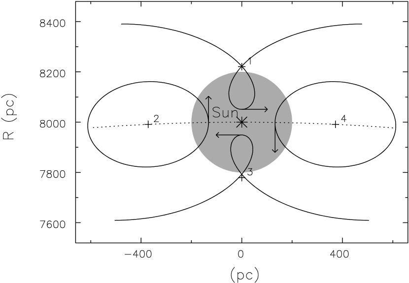
Figure 9: Four possible orbits that pass through the vicinity of the Sun (asterisk), drawn in the frame that rotates at the angular rate of the LSR. The sense of rotation of the Galaxy is clockwise, in line with the usual convention. The sample volume is the lightly shaded region, and the dotted line marks the solar circle.

Both the present sample and the GCS sample of Paper I were confined to stars that happen to lie near the Sun at present. Since stars move on eccentric orbits, most stars in the sample are merely visiting the solar vicinity from farther afield.

Fig. 9 shows four possible orbits of stars near the Sun that all happen to pass through the (shaded) survey volume. The orbits are drawn in the frame of the LSR and have sufficiently small radial excursions to approximate Lindblad epicycles. All four orbits have the same $J_{R}$ (epicycle size); those labelled 2 & 4, with guiding centres (plus symbols) lying on the solar circle, have the same $J_{\phi}\;(=L_{z})$ as does the Sun, while orbits 1 & 3 have, respectively, greater and smaller values of $J_{\phi}$. Orbits 2 & 4 are closed ellipses, because their guiding centres move at the same angular rate as the frame, but the guiding centres of the other two ellipses, which are marked at the point of the star’s closest approach to the Sun, drift relative to the LSR. For clarity, the orbits shown do not loop around the Sun so that the vectors, which show peculiar velocities relative to the LSR, appear to correlate with the direction of the star from the solar position. In reality, stars anywhere in the survey region can have peculiar velocities in any direction.

Figure 10: The distribution of angles for GCS stars. Stars with radial action $>0.05L_{z,0}$ are excluded. Note the difference in scales between the two axes.

The value of $w_{\phi}$ is the instantaneous Galactic azimuth of the guiding centre, which Sellwood (2010, Paper I) chose to be zero on the line connecting the Sun to the Galactic centre. Thus $w_{\phi}>0$ for stars ahead of the Sun. The $w_{R}$ variable is the phase of the star around its epicycle, which increases with time in the sense shown by the arrows. Again Sellwood (2010) adopted $w_{R}=0$ for a star at its apocentre and consequently $w_{R}=\pm\pi$ for a star at its pericentre. Note that action-angle variables, unlike Lindblad’s epicycles, can also be used for more eccentric orbits, for which the guiding centres generally orbit more slowly than the circular speed and the radial oscillation is anharmonic.

Fig. 4 of Paper I showed the separate distributions of $w_{R}$ and $w_{\phi}$ for stars in the GCS sample having $J_{R}<0.05L_{z,0}$. Here, Fig. 10 shows the joint distribution of the same stars in the space of both angles. The azimuthal phase distribution is confined to $|w_{\phi}|\la 0.4$ reflecting the limited spread in Galactic azimuths of the guiding centres for stars that pass through the survey volume.

The distribution of $w_{\phi}$ values for stars having $w_{R}=0$, such as orbit 3 in Fig. 9, or $w_{R}=\pm\pi$ (orbit 1) is very narrow because their guiding centres lie along the radius vector from the Galactic centre to the Sun for all values of $J_{R}$. Stars in the first quadrant of Fig. 10 are inward moving stars (because $w_{R}>0$) with guiding centres ahead of the Sun ($w_{\phi}>0$), such as orbit 4. Conversely, stars in the third quadrant ($w_{\phi}<0$) are outward moving stars having $w_{R}<0$ (e.g. orbit 2). Thus the selection criteria preclude stars from lying in the second and fourth quadrants. The spread of $w_{\phi}$ values for $w_{R}\sim\pm\pi/2$ reflects the spread in the sizes of the epicycles of the stars in the sample, from which more eccentric orbits were eliminated.

Figure 11: The distribution of $4w_{\phi}-w_{R}$ for GCS stars, which was not shown in Paper I. As there, stars with radial action $>0.05L_{z,0}$ are excluded.

Sellwood (2010) argued that a concentration of stars having a nearly constant value of $mw_{\phi}+lw_{R}$ would be an indicator of trapping in a resonance for the selected values of $l$ and $m$. Thus he searched for an excess of stars lying along lines of fixed slope with all possible intercepts in this plot, and reported the results in his Fig. 7 of Paper I for the GCS sample. The lines for inner Lindblad resonances ($l=-1$) have a positive slope in Fig. 10. Their slopes decrease as $m$ increases, causing them to become more closely parallel to the distribution near $(w_{R},w_{\phi})=(0,0)$, giving rise to a peak near $mw_{\phi}-w_{R}=0$ as $m$ increases. The distributions shown in Fig. 7 of paper I for $m=2$ and $m=3$, and in Fig. 11 of this paper, show the increasing prominence of this feature, which is purely an artefact of the sample selection. A similar feature appears near $mw_{\phi}+w_{R}=\pm\pi$ when $l=1$, since the lines have negative slope in these cases.

Sellwood (2010) drew attention to the peaks that lay away from $mw_{\phi}-w_{R}=0$ for the cases of inner Lindblad resonances. These peaks arise in part from the concentration of GCS stars near $w_{R}\sim-1.5$, $w_{\phi}\sim-0.15$ in Fig 10, but the clump is visibly extended, which McMillan (2011) described as having a triangular shape. Since the excess lies in the third quadrant, it gives rise to peaks in the distributions of $mw_{\phi}-w_{R}$ that shift closer to zero as $m$ is increased. Obviously the same excess gives rise to peaks near $mw_{\phi}+w_{R}\ga-2$ for lines of negative slope in the cases of an OLR but, at least for the GCS sample, they are not as striking as those for the ILR cases.

The case for an ILR made by Sellwood (2010) did not rest solely on this slight difference, however. He attached far greater significance to the fact that stars lying along a line of positive slope extending through the clump were exactly those that lay along the resonant scattering tongue in action space, as shown in Fig. 8 of Paper I. As this was not the case for stars lying on lines of negative slope, Sellwood concluded that an ILR was responsible. Unfortunately, McMillan (2011) found that his conclusion was compromised by selection effects: if stars are not only in the vicinity of the Sun but are also trapped in a resonance, McMillan was able to show that both ILR and OLR models give rise to features in the angle distribution (i.e., Fig. 10) having positive slope. Thus, although scattering at a Lindblad resonance was clearly established, the test in Paper I did not enable the character of the resonance to be determined.

References

- (1)
- Abazajian et al. (2009) Abazajian K. N. et al. 2009, ApJS, 182, 543
- Antoja et al. (2009) Antoja, T., Valenzuela, O., Pichardo, B., Moreno, E., Figueras, F. & Fernández, D. 2009, ApJL, 700, L78
- Bensby et al. (2007) Bensby, T., Oey, M. S., Feltzing, S. & Gustafsson, B. 2007, ApJL, 655, L89
- Binney & Tremaine (2008) Binney, J. & Tremaine, S. 2008, Galactic Dynamics 2nd Ed. (Princeton: Princeton University Press), (BT08)
- Bovy & Hogg (2010) Bovy, J. & Hogg, D. W. 2010, ApJ, 717, 617
- Breddels et al. (2010) Breddels, M. A. et al. 2010, A&A, 511, A90
- Chakrabarty (2007) Chakrabarty, D. 2007, A&A, 467, 145
- Dehnen (1998) Dehnen, W. 1998, AJ, 115, 2384
- Dehnen (2000) Dehnen, W. 2000, AJ, 119, 800
- Demarque et al. (2004) Demarque, P., Woo, J-H., Kim, Y-C. & Yi, S. K. 2004, ApJS, 155, 667
- De Simone et al. (2004) De Simone, R. S., Wu, X. & Tremaine, S. 2004, MNRAS, 350, 627
- Dotter et al. (2008) Dotter, A., Chaboyer, B., Jevremović, D., Kostov, V., Baron, E. & Ferguson, J. W. 2008, ApJS, 178, 89
- Eggen (1996) Eggen, O. J. 1996, AJ, 112, 1595
- Famaey et al. (2007) Famaey, B., Pont, F., Luri, X., Udry, S., Mayor, M. & Jorrissen, A. 2007, A&A, 461, 957
- Helmi et al. (2006) Helmi, A., Navarro, J. F., Nordström, B., Holmberg, J., Abadi, M. G. & Steinmetz, M. 2006, MNRAS, 365, 1309
- Høg et al. (2000) Høg, E., Fabricius, C., Makarov, V. V., Urban, S., Corbin, T., Wycoff, G., Bastian, U., Schwekendiek, P. & Wicenec, A. 2000, A&A, 355, L27
- Holmberg et al. (2009) Holmberg, J., Nordström, B. & Andersen, J. 2009, A&A, 501, 941
- Ivezić et al. (2008) Ivezić, Z̆. et al. 2008, ApJ, 684, 287
- Johnson & Soderblom (1987) Johnson, D. R. H. & Soderblom, D. R. 1987, AJ, 93, 864
- Jurić et al. (2008) Jurić, M. et al. 2008, ApJ, 673, 864
- Karatas & Klement (2011) Karatas, Y. & Klement, R. J. 2011, New. Astron., 17, 22
- Klement et al. (2008) Klement, R., Fuchs, B. & Rix, H.-W. 2008, ApJ, 685, 261
- Klement et al. (2011) Klement, R. J., Bailer-Jones, C. A. L., Fuchs, B., Rix, H.-W. & Smith, K. W. 2011, ApJ, 726, 103
- Lee et al. (2008) Lee, Y. S. et al. 2008, AJ, 136, 2022
- McMillan (2011) McMillan, P. J. 2011, MNRAS, in press (arXiv:1107.1384)
- Minchev et al. (2010) Minchev, I., Boily, C., Siebert, A. & Bienayme, O. 2010, MNRAS, 407, 2122
- Munn et al. (2004) Munn, J. A. et al. 2004, AJ, 127, 3034
- Munn et al. (2008) Munn, J. A. et al. 2008, AJ, 136, 895
- Nordström et al. (2004) Nordström, B., Mayor, M., Andersen, J., Holmberg, J., Pont, F., Jørgensen, B. R., Olsen, E. H., Udry, S. & Mowlavi, N. 2004, A&A, 418, 989
- Perryman et al. (2001) Perryman, M. A. C., de Boer, K. S., Gilmore, G., Høg, E., Lattanzi, M. G., Lindegren, L., Luri, X., Mignard, F., Pace, O. & de Zeeuw, P. T. 2001, A&A, 369, 339
- Piatek et al. (2002) Piatek, S., Pryor, C., Olszewski, E. W., Harris, H. C., Mateo, M., Minniti, D., Monet, D. G., Morrison, H. & Tinney, C. G. 2002, AJ, 124, 3198
- Pompéia et al. (2011) Pompéia et al. 2011, MNRAS, 415, 1138
- Quillen (2003) Quillen, A. C. 2003, AJ, 125, 785
- Quillen & Minchev (2005) Quillen, A. C. & Minchev, I. 2005, AJ, 130, 576
- Schönrich et al. (2010) Schönrich, R., Binney, J. & Dehnen, W. 2010, MNRAS, 403, 829
- Sellwood (1994) Sellwood, J. A. 1994, in Galactic and Solar System Optical Astrometry ed. L. Morrison (Cambridge: Cambridge University Press) p. 156
- Sellwood (2000) Sellwood, J. A. 2000, Ap. Sp. Sci., 272, 31 (astro-ph/9909093)
- Sellwood (2010) Sellwood, J. A. 2010, MNRAS, 409, 145 (Paper I)
- S (2006) Skrutskie, M. F. et al. 2006, AJ, 131, 1163
- Steinmetz et al. (2006) Steinmetz, M., et al. 2006, AJ, 132, 1645
- West et al. (2011) West, A. A., et al. 2011, AJ, 141, 97
- Yanny et al. (2009) Yanny, B. et al. 2009, AJ, 137, 4377
- York et al. (2000) York, D. G., et al. 2000, AJ, 120, 1579
- Zwitter et al. (2008) Zwitter, T., et al. 2008, AJ, 136, 421
- Zwitter et al. (2010) Zwitter, T., et al. 2010, A&A, 522, A54