Magneto-elastic quantum fluctuations and phase transitions in the iron superconductors

Abstract

We examine the relevance of magneto-elastic coupling to describe the complex magnetic and structural behaviour of the different classes of the iron superconductors. We model the system as a two-dimensional metal whose magnetic excitations interact with the distortions of the underlying square lattice. Going beyond mean field we find that quantum fluctuation effects can explain two unusual features of these materials that have attracted considerable attention. First, why iron telluride orders magnetically at a non-nesting wave-vector $(\pi/2,\pi/2)$ and not at the nesting wave-vector $(\pi,0)$ as in the iron arsenides, even though the nominal band structures of both these systems are similar. And second, why the $(\pi,0)$ magnetic transition in the iron arsenides is often preceded by an orthorhombic structural transition. These are robust properties of the model, independent of microscopic details, and they emphasize the importance of the magneto-elastic interaction.

Introduction.— The recently discovered iron superconductors with unusually high transition temperatures exhibit a rich phase diagram that includes structural, magnetic and superconducting transitions kamihara ; review . As such these materials are the latest playgrounds to study how in complex materials different phases compete, and how this unconventional setting eventually gives rise to superconductivity. Theoretically, one of the goals at present is to identify the microscopic interactions that give rise to the rich phase diagram. This motivates us to present a microscopic study of the simplest symmetry-allowed model Hamiltonian describing magneto-elastic interaction. The results allow us to argue that this coupling contains physics relevant for the iron superconductors, and therefore it is an important microscopic ingredient.

Crystallographically these materials have a layered structure, which is reflected in their energy bands with weak dispersion along the $c$-axis compared to that along the $ab$-plane singh ; subedi . Consequently, it is often simpler to consider them as two-dimensional systems weakly coupled along the $c$-axis. The undoped and the lightly doped compounds usually undergo magneto-structural transitions from paramagnetic metals with tetragonal crystalline symmetry to low temperature antiferromagnetic (AF) metals with either orthorhombic (in case of the FeAs systems) or monoclinic (in case of Fe_1+yTe) structures. These transitions are suppressed in favour of superconductivity when they are either doped or put under external pressure. The AF order of the FeAs systems is at the wave-vector $(\pi,0)$ in the Brillouin zone defined by the plane of the Fe atoms with 1Fe/cell, and it is often preceded in temperature by the structural transition. On the other hand, the AF order of Fe_1+yTe is at $(\pi/2,\pi/2)$, and the lattice distorts simultaneously.

While it is likely that the $(\pi,0)$ order of FeAs is a consequence of the Fermi surface nesting in these multi-band systems singh , from the perspective of a band picture there remains at least two important puzzles concerning the magneto-structural properties. First, why Fe_1+yTe, whose nominal band structure is similar to that of the FeAs systems subedi , orders at $(\pi/2,\pi/2)$ and not at the nesting wave-vector $(\pi,0)$. And second, why the AF transition of the FeAs systems is often preceded in temperature by a tetragonal-orthorhombic structural transition. The main results of this study are to show that both these features are natural consequences of quantum fluctuations induced by the magneto-elastic interaction. We find that the former property is due to spin fluctuations scattering with short wavelength phonons, and the latter is driven by critical spin fluctuations near a $(\pi,0)$ AF transition.

The above questions, as well as the general magneto-structural properties of these materials, have been addressed earlier from various points of view. Some of these are based on itinerant electron models which emphasize the physics of nested Fermi surfaces zhang-knolle ; han . There are also studies that suggest that the electron-electron interaction is strong haule-aichhorn , which justifies describing the magnetic properties by Heisenberg spin models with appropriate couplings qimiao-fang . The structural transition has been viewed as a consequence of various kinds of electron order such as orbital ordering orbital , spin nematic ordering henley-chandra at temperatures above the magnetic transition fang ; fernandes , as well as the ordering of orbital currents kang .

In the past there has been few studies of the magneto-elastic properties of the FeAs materials which concentrated on the $c$-axis motion of the As atoms, and its strong influence on the Fe-As bond and eventually on the magnetism past . These are motivated by the observation of a pressure-driven first order volume collapse transition in CaFe₂As₂, which is concomitant with the loss of magnetism kreyssig . On the other hand, a microscopic study of the influence of the $ab$-plane distortions of the lattice on the magnetic sector using an effective model is currently lacking. This is despite the fact that the in-plane distortions have an important symmetry-allowed coupling with the order parameters of the magnetic transition, which can make the transition weakly first order barzykin ; larkinpikin .

Here we perform such a microscopic study using a model Hamiltonian $\mathcal{H}_{ME}$ introduced phenomenologically in Ref. paul, , and where it was argued that a mean field treatment of $\mathcal{H}_{ME}$ describes several salient features of the magneto-structural transitions in the FeAs cano and Fe_1+yTe paul systems. In the case of FeAs it explains (i) why the magnetic and structural transitions are separate in some materials while they are concomitant in others, (ii) why the transitions appear to be first order in some cases even though they are allowed to be second order from a symmetry point of view, and (iii) why the systems prefer a collinear magnetic state instead of a non-collinear order cano . In the case of Fe_1+yTe it explains why in the magnetic phase the system undergoes a uniform monoclinic distortion, and a modulated one with wave-vector $(\pi,\pi)$ such that the Fe-Fe bonds are alternately elongated and shortened paul . Our aim here is to go beyond mean field, and to study the quantum fluctuations of the elastic and the magnetic degrees of freedom and thereby examine further the relevance of $\mathcal{H}_{ME}$.

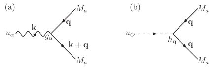
Figure 1: Magneto-elastic coupling [Eq. (1)] describing scattering of paramagnons (straight line) (a) with phonons (wavy line) at finite ${\bf k}$, and (b) with orthorhombic distortion (dash line) at ${\bf k}\rightarrow 0$ limit. The associated matrix elements $g_{\alpha}({\bf k},{\bf q})$ and $h({\bf q})$ are defined in Eqs. (2) and (3) respectively.

Model.— We consider a two-dimensional metal on a square lattice with magnetic and elastic degrees of freedom that are coupled by the Hamiltonian

$$\mathcal{H}_{ME}=\lambda_{0}\sum_{\langle ij\rangle}\left({\bf u}_{i}-{\bf u}_{j}\right)\cdot\hat{n}_{ij}\left({\bf M}_{i}\cdot{\bf M}_{j}\right).$$ (1)

Here $\lambda_{0}$ is the coupling constant with dimension of energy per length, ${\bf u}_{i}\equiv{\bf u}({\bf r}_{i})$ is the displacement of the Fe atom from its equilibrium position at ${\bf r}_{i}$, $\langle ij\rangle$ implies nearest neighbour sites, $\hat{n}_{ij}$ is the unit vector along the $i-j$ bond, and ${\bf M}_{i}$ is the local magnetization at ${\bf r}_{i}$. We neglect spin-orbit coupling, and magneto-elastic terms of $\mathcal{O}(u^{2})$ and higher. In the context of insulating magnets $\mathcal{H}_{ME}$ describes the variation $\partial J/\partial r$ of the Heisenberg exchange $J$ with bond length, and its effects are well-studied becca-penc . In the case of metals, where such couplings are far less studied, $\mathcal{H}_{ME}$ describes the bond-length dependence of the parameter $V_{ij}$ that characterize the nearest neighbour interaction $V_{ij}\rho_{i\uparrow}\rho_{j\downarrow}$, with $\rho_{i\sigma}$ being the density of electrons with spin $\sigma$ at site $i$.

We study the system from the paramagnetic side, and we approximate ${\bf M}_{i}$ to be $O(3)$ variables describing spin fluctuations (paramagnons). Conceptually, they can be introduced as Hubbard-Stratonovich fields to decouple the appropriate electron-electron interaction, after which the electrons can be integrated out moriya . The resulting action for the magnetic sector can be written as $S_{M}=\sum_{{\bf q},\nu_{n},a}\chi_{0}^{-1}({\bf q},\nu_{n})M^{\ast}_{a}({\bf q},\nu_{n})M_{a}({\bf q},\nu_{n}),$ where $a=(x,y,z)$ in $O(3)$ space, ${\bf M}({\bf q})$ is the Fourier transform of ${\bf M}({\bf r}_{i})$, and $\nu_{n}$ is a bosonic Matsubara frequency. We assume that the paramagnon propagator describes damped dynamics with $\chi_{0}^{-1}({\bf q},\nu_{n})=\Pi_{0}({\bf q})+\left|\nu_{n}\right|,$ and having the bare dispersion $\Pi_{0}({\bf q})=\Omega_{0}+\Omega_{1}[\cos q_{x}\cos q_{y}-(\cos 2q_{x}+\cos 2q_{y})/8]$ with $\Omega_{0}>\Omega_{1}>0$. With this choice $\Pi_{0}({\bf q})$ has a global minima at ${\bf q}=(\pi,0)$ (and at the symmetry related points) which models the nesting property of the underlying Fermi surface. The approach towards the magnetic instability can be described by lowering $\Omega_{0}$.

As our results are independent of the microscopic details of the elastic sector, it is sufficient to describe it using the simplest model compatible with the square symmetry. The lattice variables are defined by the strain tensor $\epsilon_{\alpha\beta}({\bf r}_{i})=u_{\alpha\beta}+i/2\sum_{{\bf k}\neq 0}[k_{\alpha}u_{\beta}({\bf k})+\alpha\leftrightarrow\beta]\exp(i{\bf k}\cdot{\bf r}_{i}),$ where $\alpha,\beta=(x,y)$ in two dimensions. This includes the uniform strains $u_{\alpha\beta}$, and the phonons described by ${\bf u}({\bf k})$ which is the Fourier transform of ${\bf u}({\bf r}_{i})$ larkinpikin . The energy per unit area due to $u_{\alpha\beta}$ is given by $E_{S}=C_{11}(u_{xx}+u_{yy})^{2}/2+C_{12}u_{xx}u_{yy}+C_{66}u_{xy}^{2}/2,$ where the $C$s are the elastic constants in Voigt notation. The order parameter for the tetragonal-orthorhombic transition is $u_{o}\equiv u_{xx}-u_{yy}$, and the associated elastic constant is $C_{o}\equiv(C_{11}-C_{12})/2$. Next, the phonons are described by the action $S_{P}=\sum_{{\bf k},\nu_{n},\mu}D_{\mu}^{-1}({\bf k},\nu_{n})u^{\ast}_{\mu}({\bf k},\nu_{n})u_{\mu}({\bf k},\nu_{n}),$ where $\mu$ is the polarization index. We assume the propagator to have the standard form $D_{\mu}^{-1}({\bf k},\nu_{n})=-2\omega_{{\bf k}\mu}/(\nu_{n}^{2}+\omega^{2}_{{\bf k}\mu})$, with $\omega_{{\bf k}\mu}$ the phonon dispersion. We obtain it from a harmonic theory in which the eigenvalues of the dynamical matrix $N_{\alpha\beta}({\bf k})$ give $m\omega^{2}_{{\bf k}\mu}$, $m$ being the atomic mass of Fe. We take $N_{xx}=4C_{11}\sin^{2}(k_{x}/2)+C_{66}\sin^{2}(k_{y}/2)$, $N_{yy}=N_{xx}(x\leftrightarrow y)$, and $N_{xy}=N_{yx}=(4C_{12}+C_{66})\sin(k_{x}/2)\sin(k_{y}/2)$. Thus, the elastic sector is entirely characterized by the $C$s and $m$.

Before performing the calculations it is instructive to re-write the interaction in Fourier space as

$$\mathcal{H}_{ME}=2i\lambda_{0}\sum_{\alpha,a,{\bf k},{\bf q}}g_{\alpha}({\bf k},{\bf q})u_{\alpha}({\bf k})M^{\ast}_{a}({\bf k}+{\bf q})M_{a}({\bf q}),$$

where $g_{\alpha}({\bf k},{\bf q})$ are matrix elements with

$$g_{\alpha}({\bf k},{\bf q})=\sin(k_{\alpha}+q_{\alpha})-\sin(q_{\alpha}).$$ (2)

They play an important role due to the property that $g_{\alpha}\rightarrow 0$ as $k\rightarrow 0$, which implies that the coupling to the phonons vanishes in the limit of uniform displacements. In this limit the paramagnons couple to the classical variables $u_{\alpha\beta}$, and in particular the coupling to $u_{o}$ is associated with the matrix element

$$h({\bf q})=\cos q_{x}-\cos q_{y}.$$ (3)

The coupling of the paramagnons to the phonons (${\bf k}\neq 0$) and to $u_{o}$ (${\bf k}\rightarrow 0$) along with their respective matrix elements are shown graphically in Fig. 1.

As our model is two dimensional, strictly speaking it cannot be used to study the finite temperature magnetic transition due to the Mermin-Wagner theorem. In the following our strategy is to perform calculations at zero temperature ($T$) where the theorem is inapplicable, and to infer finite-$T$ consequences using adiabaticity argument. In general, at finite-$T$ the magnitude of the results below are enhanced due to the thermal fluctuations.

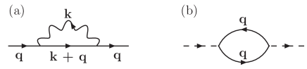
Figure 2: Magneto-elastic coupling induced quantum fluctuations producing (a) static paramagnon self-energy $\Pi_{2}({\bf q})$ due to scattering with phonons, and (b) correction to the orthorhombic elastic constant $C_{o}$ due to paramagnons.

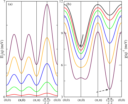
Figure 3: (colour online). (a) Paramagnon self-energy $\Pi_{2}({\bf q})$ along the high symmetry directions of the Brillouin zone for increasing values of magneto-elastic coupling $\lambda_{0}=1,\cdots,5$ (bottom to top) in unit of 10 meV/Å. It is always peaked at $(\pi/2,\pi/2)$. (b) The corresponding renormalized paramagnon dispersions $\chi^{-1}({\bf q})=\Pi_{0}({\bf q})-\Pi_{2}({\bf q})$ (second-from-top to bottom curves respectively), and the bare dispersion $\Pi_{0}({\bf q})$ (topmost curve, shifted up by 0.2 meV for clarity). At large enough $\lambda_{0}$ (bottom-most) the global minima changes to $(\pi/2,\pi/2)$ (dash arrow) from the nesting driven $(\pi,0)$ wave-vector (solid arrow).

Results.— (i) First we examine the static paramagnon self-energy obtained due to virtual scattering with the phonons. This is given by (see Fig. 2a)

$$\Pi_{2}({\bf q}) = -4\lambda_{0}^{2}T\sum_{{\bf k},\nu_{n},\alpha,\beta,\mu}(2m\omega_{{\bf k}\mu})^{-1}g_{\alpha}({\bf k},{\bf q})g_{\beta}({\bf k},{\bf q})$$

$$\times \epsilon_{\mu}^{\alpha}({\bf k})\epsilon_{\mu}^{\beta}({\bf k})D_{\mu}({\bf k},i\nu_{n})\chi_{0}({\bf k}+{\bf q},i\nu_{n}),$$

where $\hat{\epsilon}_{\mu}({\bf k})$ are the polarization vectors. We perform the ${\bf k}$-sum numerically, taking $(\Omega_{0},\Omega_{1})=(10,2)$ meV (the precise value of these parameters do not affect the result qualitatively). We also use $(C_{11},C_{12},C_{66})=(0.484,0.161,0.141)$ $10^{4}$ meV/Ų from elastic constant measurements on BaFe₂As₂ yoshizawa suitably normalized for two dimensions. In Fig. 3a we plot $\Pi_{2}({\bf q})$ along high symmetry directions of the Brillouin zone for various values of the coupling $\lambda_{0}$. Note that the magnitude of $\Pi_{2}({\bf q})$ increases with $\lambda_{0}$ as expected, but more importantly, it is peaked at $(\pi/2,\pi/2)$ for all $\lambda_{0}$ (below we explain why). The consequence of this property is demonstrated in Fig. 3b where we show the corresponding renormalized paramagnon dispersions (second-from-top to bottom curves) given by $\chi^{-1}({\bf q})=\Pi_{0}({\bf q})-\Pi_{2}({\bf q}),$ as well as the bare dispersion $\Pi_{0}({\bf q})$ for comparison (topmost curve). Since $\Pi_{2}({\bf q})$ is always peaked at $(\pi/2,\pi/2)$, for $\lambda_{0}>\lambda_{0}^{\ast}$ (e.g., the bottommost curve in Fig. 3b) the global minima of $\chi^{-1}({\bf q})$ changes from the nesting driven wave-vector $(\pi,0)$ to the magneto-elastic coupling driven wave-vector $(\pi/2,\pi/2)$. This implies that in this model the magnetic instability is at $(\pi/2,\pi/2)$ for sufficiently large $\lambda_{0}$. Thus, the $(\pi/2,\pi/2)$ magnetic order observed in Fe_1+yTe can be explained as a signature of strong magneto-elastic coupling, while in the FeAs systems this effect is presumably weaker and the nesting driven $(\pi,0)$ instability is preferred. Indeed, several authors have argued that the electron-electron interaction effects, which favours the magneto-elastic coupling, is stronger in Fe_1+yTe than in the FeAs systems review ; orbital .

The above result can be understood simply from the following argument. Since $g_{\alpha}$ vanishes for $k\rightarrow 0$, the ${\bf k}$-sum above is dominated by large $k$ (short wavelength phonons), and typically $\omega_{{\bf k}\mu}\sim E_{0}$ the phonon bandwidth, which is the largest energy scale in the model. Thus, $T\sum_{\nu_{n}}D_{\mu}({\bf k},i\nu_{n})\chi_{0}({\bf k}+{\bf q},i\nu_{n})\sim 1/E_{0},$ and its ${\bf q}$-dependence is negligible. Therefore, the dominant ${\bf q}$-dependence of $\Pi_{2}({\bf q})$ is from the matrix elements $g_{\alpha}g_{\beta}$. Then a simple power counting argument, and the fact that in a stable lattice the diagonal components of $N_{\alpha\beta}$ are larger than the off-diagonal ones, establishes that

$$\Pi_{2}({\bf q})=A+B\left(\sin^{2}q_{x}+\sin^{2}q_{y}\right)-C\cos q_{x}\cos q_{y},$$ (4)

with $A,B>C>0$. Note that this result is independent of the details of the paramagnon and the phonon dispersions, and its main ingredient is the fact that $\mathcal{H}_{ME}$ involves the nearest neighbour sites. Including couplings with longer range will not change the result provided they are smaller in magnitude compared to $\lambda_{0}$. This is plausible, since the electron-electron interaction is expected to reduce with distance. However, it needs to be checked using first principles calculation. Note also that the value of $\lambda_{0}^{\ast}$ depends intricately on the microscopic details. In particular, it depends on the relative strength of the nesting driven minimum at $(\pi,0)$, and on the magnitude of the longer range magneto-elastic couplings.

(ii) Next we compute the correction to the orthorhombic elastic constant $C_{o}$ due to quantum fluctuations of the paramagnons which is given by (see Fig. 2b)

$$\delta C_{o}=-3\lambda_{0}^{2}T\sum_{{\bf q},\nu_{n}}h^{2}({\bf q})\chi_{0}^{2}({\bf q},i\nu_{n}).$$

For two dimensional spin fluctuations in the vicinity of a $(\pi,0)$ magnetic instability (which is tuned by $\Omega_{0}$) we get

$$\delta C_{o}=-4\lambda_{0}^{2}/(\pi^{2}\Omega_{1})\log(1/\delta),$$ (5)

where $\delta=(\Omega_{0}-\Omega_{\rm cr})/\Omega_{1}$ measures the closeness to the magnetic instability at $\Omega_{0}=\Omega_{\rm cr}$. This implies that, before the system becomes magnetic ($\Omega_{0}>\Omega_{\rm cr}$), the renormalized elastic constant $(C_{o}+\delta C_{o})$ vanishes and the system encounters an orthorhombic instability. This softening of the lattice with $\delta C_{0}\propto\log(1/\chi_{m})$, where $\chi_{m}$ is the dimensionless static magnetic susceptibility at $(\pi,0)$, is in principle verifiable from neutron scattering data and from elastic constant measurements. A similar softening of $C_{0}$ due to nematic fluctuations is discussed in Ref. fernandes, . Using adiabaticity argument it is possible to extend the phase boundaries to finite temperatures in the $T-\Omega_{0}$ plane, and the resulting phase diagram shows that the magnetic transition is preceded in temperature by the orthorhombic instability. However, close enough to the finite-$T$ magnetic transition the critical theory is non-Gaussian, and the quantitative aspects of the current treatment becomes invalid.

In practice, even at $T=0$ and in three dimensions the log divergence is cutoff by the paramagnon dispersion along the $c$-axis, and the precise fate of the structural instability depends on microscopic details. Nevertheless, for quasi-two dimensional paramagnons one should expect considerable orthorhombic softening, and therefore this mechanism explains why often (but not always) the $(\pi,0)$ magnetic transition in the FeAs systems is accompanied by an orthorhombic transition. In passing we note that a similar monoclinic softening is expected near a $(\pi/2,\pi/2)$ magnetic transition (and can be relevant for Fe_1+yTe), but to capture this physics one needs to generalize $\mathcal{H}_{ME}$ and include next-nearest neighbour couplings.

Conclusion.— We studied the effects of quantum fluctuations induced by magneto-elastic coupling [Eq. (1)] in a two-dimensional metal on a square lattice. The coupling describes the simplest symmetry-allowed scattering between the paramagnons and the distortions of the lattice. At a qualitative level the model explains (i) why Fe_1+yTe orders magnetically at $(\pi/2,\pi/2)$ and not at the nesting wave-vector $(\pi,0)$, and (ii) why the FeAs systems often undergo an orthorhombic transition in the vicinity of the $(\pi,0)$ magnetic transition. The former result is due to paramagnons scattering with short wavelength phonons, and the latter is driven by the critical spin fluctuations. We hope these results will stimulate further studies of the coupling using a more realistic model and in conjunction with first principles calculations. Such couplings can give rise to qualitatively new physics, and they can be relevant for correlated metals in general.

The author is very thankful to E. Boulat, A. Cano, H. Capellmann, E. Kats, I. Vekhter, and T. Ziman for insightful discussions.

References

- (1) Y. Kamihara et. al., J. Am. Chem. Soc. 130, 3296 (2008).
- (2) For reviews see, e.g., M. Norman, Physics 1, 21 (2008); D. C. Johnston, Adv. Phys. 59, 803 (2010).
- (3) D. J. Singh and M.-H. Du, Phys. Rev. Lett. 100, 237003 (2008)
- (4) A. Subedi et al., Phys. Rev. B 78, 134514 (2008).
- (5) See, e.g., Y.-Z. Zhang et al., Phys. Rev. B 81, 094505 (2010); J. Knolle et al., ibid 81, 140506(R) (2010); V. Cvetkovic and Z. Tesanovic, ibid 80, 024512 (2009).
- (6) M. J. Han and S. Y. Savrasov, Phys. Rev. Lett. 103, 067001 (2009).
- (7) K. Haule, G. Kotliar, New J. Phys. 11, 025021 (2009); M. Aichhorn et al., Phys. Rev. B 82, 064504 (2010).
- (8) Q. Si and E. Abrahams, Phys. Rev. Lett. 101, 076401 (2008); C. Fang et al., Europhys. Lett. 86, 67005 (2009).
- (9) See, e.g., F. Krüger et al., Phys. Rev. B 79, 054504 (2009); A. Turner at al., ibid 80, 224504 (2009), W. Lv et al., ibid 80, 224506 (2009).
- (10) C. L. Henley, Phys. Rev. Lett. 62, 2056 (1989); P. Chandra et al., ibid 64, 88 (1990).
- (11) C. Fang et. al., Phys. Rev. B 77, 224509 (2008).
- (12) R. M. Fernandes et al., Phys. Rev. Lett. 105, 157003 (2010).
- (13) J. Kang and Z. Tešanović, Phys. Rev. B 83, 020505(R) (2011).
- (14) T. Yildirim, Phys. Rev. Lett. 102, 037003 (2009); M. L. Kulić and A. A. Haghighirad, Europhys. Lett. 87, 17007 (2009); A. Hackl and M. Vojta, New J. Phys. 11, 055064 (2009); T. Egami et al., Physica C 470, S294 (2010).
- (15) A. Kreyssig et al., Phys. Rev. B 78, 184517 (2008).
- (16) V. Barzykin and L. P. Gorkov, Phys. Rev. B 79, 134510 (2009).
- (17) A. I. Larkin and S. A. Pikin, Sov. Phys. JETP 29, 891 (1969).
- (18) I. Paul et al., Phys. Rev. B 83, 115109 (2011).
- (19) A. Cano et al., Phys. Rev. B 82, 020408(R) (2010).
- (20) See, e.g., F. Becca and F. Mila, Phys. Rev. Lett. 89, 037204 (2002); K. Penc et al., ibid 93, 197203 (2004).
- (21) T. Moriya, Spin fluctuations in itinerant electron magnets (Springer-Verlag, Berlin 1985).
- (22) M. Yoshizawa et al., arXiv:1008.1479.