xx xx A Information Theory and Its Applications [kenta@comm.ss.titech.ac.jp]Kenta KASAImTITECH [sakaniwa@ss.titech.ac.jp]Kohichi SAKANIWAfTITECH [TITECH]Dept. of Communications and Integrated Systems, Tokyo Institute of Technology 2-12-1, O-Okayama, Meguro-ku, Tokyo, 152-8550, Japan

Spatially-Coupled MacKay-Neal Codes and Hsu-Anastasopoulos Codes

Kudekar et al. recently proved that for transmission over the binary erasure channel (BEC), spatial coupling of LDPC codes increases the BP threshold of the coupled ensemble to the MAP threshold of the underlying LDPC codes. One major drawback of the capacity-achieving spatially-coupled LDPC codes is that one needs to increase the column and row weight of parity-check matrices of the underlying LDPC codes.

It is proved, that Hsu-Anastasopoulos (HA) codes and MacKay-Neal (MN) codes achieve the capacity of memoryless binary-input symmetric-output channels under MAP decoding with bounded column and row weight of the parity-check matrices. The HA codes and the MN codes are dual codes each other.

The aim of this paper is to present an empirical evidence that spatially-coupled MN (resp. HA) codes with bounded column and row weight achieve the capacity of the BEC. To this end, we introduce a spatial coupling scheme of MN (resp. HA) codes. By density evolution analysis, we will show that the resulting spatially-coupled MN (resp. HA) codes have the BP threshold close to the Shannon limit.

1 Introduction

Achieving the capacity of memoryless binary-input symmetric-output (MBS) channels [1, Chap. 4] under efficient decoding algorithms used to be an ultimate goal for coding theorists. The capacity of MBS channels was practically achieved by irregular LDPC codes [1] with belief propagation (BP) decoding and rigorously achieved by polar codes [2] with successive cancellation. Spatially-coupled (SC) LDPC codes [3] have bounded range of parity-check constrains like convolutional codes. Recently, SC-LDPC codes have attracted much attention due to the fact that the codes achieves the capacity of binary erasure channels (BEC) [3] and an observation that the codes seem to achieve the capacity of MBS channels [4].

SC-LDPC codes are capacity-achieving codes designed based on the construction of convolutional LDPC codes. Felström and Zigangirov [5] introduced a construction method of $({\mathtt{l}},{\mathtt{r}})$-regular convolutional LDPC codes from $({\mathtt{l}},{\mathtt{r}})$-regular block LDPC codes [1]. The convolutional LDPC codes exhibited better decoding performance than the underlying block LDPC codes under a fair comparison with respect to the code length. Note that in this paper, convolutional LDPC codes are defined by sparse band parity-check matrices. Lentmaier et al.  observed that (4,8)-regular convolutional LDPC codes exhibited the decoding performance surpassing the BP threshold of (4,8)-regular block LDPC codes [6]. Sridharan et al.  developed the density evolution (DE) [1] for the BEC and calculated the BP threshold [7]. Lentmaier et al.  developed the DE for the binary-input memoryless (BMS) channels [8]. Further, the BP threshold equals to the MAP threshold of the underlying block LDPC codes with a lot of accuracy. The MAP threshold was calculated by the extended BP (EBP) extrinsic information transfer (EXIT) function analysis [9]. Constructing convolutional LDPC codes from a block LDPC code improves the BP threshold up to the MAP threshold of the underlying codes.

Kudekar et al.  named this phenomenon “threshold saturation” and proved rigorously for the BEC [3]. In the limit of large $L$ and $w$, the SC-LDPC code ensemble $({\mathtt{l}},{\mathtt{r}},L,w)$ [3] was shown to achieve the MAP threshold of $({\mathtt{l}},{\mathtt{r}})$-regular LDPC code ensemble. The parameters $L$ and $w$ are the coupling number and the randomized window size. For more details, we refer the readers to [3].

Further, by computing EBP generalized EXIT (GEXIT) curves [9], Kudekar et al.  [4] observed empirical evidence which supports the threshold saturation occurs also for the BMS channels. For arbitrary BMS channels, the MAP threshold of the codes quickly converge to the Shannon limit while the BP threshold goes to 0 [10]. In other words, in the limit of large ${\mathtt{l}}$ as keeping $\frac{{\mathtt{l}}}{{\mathtt{r}}}$, $L$ and $w$, the SC-LDPC code ensemble $({\mathtt{l}},{\mathtt{r}},L,w)$ achieves universally the capacity of the BMS channels under BP decoding. Such universality is not supported by other efficiently-decodable capacity-achieving codes, i.e., polar codes [2] and irregular LDPC codes [11]. According to the channel, polar codes need selection of frozen bits [12] and irregular LDPC codes need optimization of degree distributions.

One major drawback of the $({\mathtt{l}},{\mathtt{r}},L,w)$ code ensemble is that one needs to increase degree ${\mathtt{l}}$ and ${\mathtt{r}}$ to strictly achieve the capacity. The number of non-zero entries in the parity-check matrices is proportional to the decoding computations of BP decoding. Specifically, for the BEC case, this is identical to the total computations for decoding [13]. The number of edges per information bit is called density. For example the density of $({\mathtt{l}},{\mathtt{r}})$-regular LDPC codes is $\frac{{\mathtt{l}}{\mathtt{r}}}{{\mathtt{r}}-{\mathtt{l}}}$. For fixed $R=1-\frac{{\mathtt{l}}}{{\mathtt{r}}}$, the density is unbounded as ${\mathtt{l}},{\mathtt{r}}\to\infty$. It is desired to reduce the density. Lentmaier et al. constructed coupled Accumulate-Repeat-Jagged-Accumulate (ARJA) codes [14] which exhibit very good BP threshold. The density of the ARJA code is bounded but the BP threshold leaves a small gap to the Shannon limit.

For any code achieving a fraction $1-\epsilon$ of capacity of the BMS under MAP decoding, Sason and Urbanke showed that the density of the code is at least $\frac{K_{1}+\ln\frac{1}{\epsilon}}{K_{2}}$, where $K_{1}$ and $K_{2}$ are constant [15]. In other words, the density of capacity-achieving codes needs to be unbounded. However, this is not the case for the codes with puncture. The punctured bits work as auxiliary states and help decoding. Such puncturing is widely used for structured codes [16]. Pfister and Sason constructed Accumulate-Repeat-Accumulate (ARA) codes and Accumulate-LDPC (ALDPC) codes which achieve the capacity of BEC with bounded density [17].

MacKay-Neal codes [18] are non-systematic two-edge type LDPC codes [16, 1]. The MacKay-Neal (MN) codes are conjectured to achieve the capacity of BMS channels under ML decoding. Murayama et al. [19] and Tanaka et al. [20] reported the empirical evidence of the conjecture for BSC and AWGN channels, respectively by a non-rigorous statistical mechanics approach known as replica method.

Hsu and Anastasopoulos [21] rigorously proved that LDPC codes concatenated with LDGM (low-density generator-matrix) codes [22] achieve the capacity of arbitrary BMS channels with bounded density under ML decoding. We name the codes Hsu-Anastasopoulos (HA) codes after the inventors. Furthermore, Wainwright and Martinian showed HA codes achieve the rate-distortion bound for symmetric Bernoulli sources [23].

On the contrary to their ML decoding performance, it is interesting to see that the MN and HA codes have no BP thresholds. In other words, the bit error rate under BP decoding does not go to 0, even if none of the transmitted bits are erased.

The aim of this paper is to present an empirical evidence that SC-MN (resp. SC-HA) codes with bounded density achieve the capacity of the BEC. To this end, we introduce a spatial coupling scheme of MN (resp. HA) codes. Spatial coupling of MN and HA codes has never been studied before. By DE analysis, we will show that the resulting SC-MN (resp. SC-HA) codes have the BP threshold close to the Shannon limit.

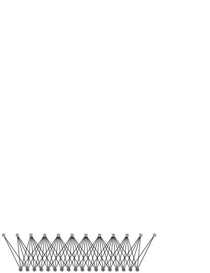
Figure 1: Protograph of $(4,8,4)$ SC-LDPC codes

2 Preliminaries

In this section, we briefly review the $({\mathtt{l}},{\mathtt{r}},L)$ SC-LDPC codes introduced by Kudekar et al. [3] and their results of performance analysis. We assume $\frac{{\mathtt{r}}}{{\mathtt{l}}}=:{\mathtt{k}}\in\mathbb{Z}.$ For simplicity, we focus on rate 1/2 codes, i.e., ${\mathtt{k}}=2$.

The SC-LDPC codes are defined by the following protograph codes [24]. The adjacency matrix of the protograph is referred to as a base matrix. The base matrix of (${\mathtt{l}},{\mathtt{r}},L$) SC-LDPC code is given as follow. Let us define as $\hat{L}:=2L+1$. Let $H({\mathtt{l}},{\mathtt{r}},\hat{L},{\mathtt{k}})$ be an $(\hat{L}+{\mathtt{l}}-1)\times{\mathtt{k}}\hat{L}$ band binary matrix of band size ${\mathtt{r}}\times{\mathtt{l}}$ and column weight ${\mathtt{l}}$, where the band size is height $\times$ width of the band. For example $H(4,8,9,2)$ is given in Fig. 2. The $({\mathtt{l}},{\mathtt{r}},L)$ SC-LDPC codes is defined as protograph codes defined by base matrix $H({\mathtt{l}},{\mathtt{r}},\hat{L},{\mathtt{k}})$. Figure 1 shows protograph of $(4,8,4)$ SC-LDPC codes. The protograph of $({\mathtt{l}},{\mathtt{r}},L)$ SC-LDPC codes have ${\mathtt{k}}\hat{L}$ variable nodes and $\hat{L}+{\mathtt{l}}-1$ check nodes. Hence, the design coding rate of $({\mathtt{l}},{\mathtt{r}},L)$ SC-LDPC codes is given by

$$R({\mathtt{l}},{\mathtt{r}},L) =\frac{{\mathtt{k}}\hat{L}-(\hat{L}+{\mathtt{l}}-1)}{{\mathtt{k}}\hat{L}}=\frac{{\mathtt{k}}-1}{{\mathtt{k}}}-\frac{{\mathtt{l}}-1}{{\mathtt{k}}\hat{L}},$$

which converges to $({\mathtt{k}}-1)/{\mathtt{k}}$ as $\hat{L}\to\infty$ with vanishing gap like $O(1/\hat{L}).$

Table 2 shows BP threshold values $\epsilon_{\mathrm{BP}}({\mathtt{l}},{\mathtt{r}},L)$ of $({\mathtt{l}},{\mathtt{r}},L)$ SC-LDPC codes. As $L$ increases, it is observed that the design coding rate $R(3,6,L)$ converges to 1/2 and the BP threshold values $\epsilon_{\mathrm{BP}}$ approach the MAP threshold value of $(3,6)$ LDPC codes $\epsilon_{\mathrm{MAP}}({\mathtt{l}},{\mathtt{r}})\approx 0.488151$.

Kudekar et al. observed $\epsilon_{\mathrm{BP}}({\mathtt{l}},{\mathtt{r}},L)$ does not converge to $\epsilon_{\mathrm{MAP}}({\mathtt{l}},{\mathtt{r}})$. There remains a small gap of order $10^{-6}$ in significant digits. In order to decrease the gap, Kudekar et al. introduced the $({\mathtt{l}},{\mathtt{r}},L,w)$ SC-LDPC codes that allows randomized connection of edges of window size $w$ [3]. It is shown that $\epsilon_{\mathrm{BP}}({\mathtt{l}},{\mathtt{r}},L,w)$ converges to $\epsilon_{\mathrm{MAP}}({\mathtt{l}},{\mathtt{r}})$ as $L$ and $w$ tend to infinity as

$$\lim_{w\to\infty}\lim_{L\to\infty}\epsilon_{\mathrm{MAP}}({\mathtt{l}},{\mathtt{r}},L,w)=\epsilon_{\mathrm{MAP}}({\mathtt{l}},{\mathtt{r}}).$$

It is known [3] that $\epsilon_{\mathrm{MAP}}({\mathtt{l}},{\mathtt{r}})$ quickly converges to the Shannon limit $1-R$, i.e.,

$$\lim_{\begin{subarray}{c}R=1-{\mathtt{l}}/{\mathtt{r}}\\ {\mathtt{l}}\to\infty\end{subarray}}\epsilon_{\mathrm{MAP}}({\mathtt{l}},{\mathtt{r}})=1-R.$$

Table 1 shows the MAP threshold values of $({\mathtt{l}},{\mathtt{r}})$ LDPC codes.

Table 1: The BP and MAP threshold values of $({\mathtt{l}},{\mathtt{r}})$ LDPC codes. The MAP threshold $\epsilon_{\mathrm{MAP}}({\mathtt{l}},{\mathtt{r}})$ quickly converges to the Shannon limit $1-R$. While the BP threshold converges to 0.

$({\mathtt{l}},{\mathtt{r}})$	$\epsilon_{\mathrm{BP}}$	$\epsilon_{\mathrm{MAP}}$
(3,6)	0.4294	0.48815
(4,8)	0.3834	0.49774
(5,10)	0.3416	0.49949
(6,12)	0.3075	0.49988
(7,14)	0.2797	0.49997

This implies that SC-LDPC codes achieve the capacity of the BEC, in the limit of large column and row weight. On the other hand, infinite column and row weight are required for the codes to achieve the capacity.

Table 2: BP threshold values $\epsilon_{\mathrm{BP}}$ of $(3,6,L)$ SC-LDPC and design coding rate $R$ [3]

$L$	$\epsilon_{\mathrm{BP}}$	$R$
1	0.714309	0.166667
2	0.587842	0.300000
4	0.512034	0.388889
8	0.488757	0.441176
16	0.488151	0.469697
32	0.488151	0.484615
64	0.488151	0.492248
128	0.488151	0.496109

3 Bounded-Density Codes Achieving Capacity under ML Decoding

In this section, we give the definition of MN codes and HA codes.

3.1 MacKay-Neal codes

Let $H_{1}$ be a random binary matrix of size $N\times\frac{{\mathtt{r}}}{{\mathtt{l}}}N$ with column weight ${\mathtt{l}}$ and row weight ${\mathtt{r}}$. Let $H_{2}$ be a random binary matrix of size $N\times N$ with column weight ${\mathtt{g}}$ and row weight ${\mathtt{g}}$.

$H(4,8,9,2)=\left[\begin{minipage}{76.82234pt} \begin{tabular}[]{@{}l@{}l@{}l@{}l@{}l@{}l@{}l@{}l@{}l@{}l@{}l@{}l@{}l@{}l@{}l@{}l@{}l@{}l}1&1&&&&&&&&&&&&&&&&\\ 1&1&1&1&&&&&&&&&&&&&&\\ 1&1&1&1&1&1&&&&&&&&&&&&\\ 1&1&1&1&1&1&1&1&&&&&&&&&&\\ &&1&1&1&1&1&1&1&1&&&&&&&&\\ &&&&1&1&1&1&1&1&1&1&&&&&&\\ &&&&&&1&1&1&1&1&1&1&1&&&&\\ &&&&&&&&1&1&1&1&1&1&1&1&&\\ &&&&&&&&&&1&1&1&1&1&1&1&1\\ &&&&&&&&&&&&1&1&1&1&1&1\\ &&&&&&&&&&&&&&1&1&1&1\\ &&&&&&&&&&&&&&&&1&1\end{tabular} \end{minipage}\right],S(5,18)=\left[\begin{minipage}{76.82234pt} \begin{tabular}[]{@{}l@{}l@{}l@{}l@{}l@{}l@{}l@{}l@{}l@{}l@{}l@{}l@{}l@{}l@{}l@{}l@{}l@{}l}1&&&&&&&&&&&&&&&&&\\ 1&1&&&&&&&&&&&&&&&&\\ 1&1&1&&&&&&&&&&&&&&&\\ 1&1&1&1&&&&&&&&&&&&&&\\ 1&1&1&1&1&&&&&&&&&&&&&\\ &1&1&1&1&1&&&&&&&&&&&&\\ &&1&1&1&1&1&&&&&&&&&&&\\ &&&1&1&1&1&1&&&&&&&&&&\\ &&&&1&1&1&1&1&&&&&&&&&\\ &&&&&1&1&1&1&1&&&&&&&&\\ &&&&&&1&1&1&1&1&&&&&&&\\ &&&&&&&1&1&1&1&1&&&&&&\\ &&&&&&&&1&1&1&1&1&&&&&\\ &&&&&&&&&1&1&1&1&1&&&&\\ &&&&&&&&&&1&1&1&1&1&&&\\ &&&&&&&&&&&1&1&1&1&1&&\\ &&&&&&&&&&&&1&1&1&1&1&\\ &&&&&&&&&&&&&1&1&1&1&1\\ &&&&&&&&&&&&&&1&1&1&1\\ &&&&&&&&&&&&&&&1&1&1\\ &&&&&&&&&&&&&&&&1&1\\ &&&&&&&&&&&&&&&&&1\end{tabular} \end{minipage}\right],V(8,4,8,2)=\left[\begin{minipage}{34.14322pt} \begin{tabular}[]{@{}l@{}l@{}l@{}l@{}l@{}l@{}l@{}l}1&&&&&&&\\ 1&&&&&&&\\ 1&1&&&&&&\\ 1&1&&&&&&\\ 1&1&1&&&&&\\ 1&1&1&&&&&\\ 1&1&1&1&&&&\\ 1&1&1&1&&&&\\ &1&1&1&1&&&\\ &1&1&1&1&&&\\ &&1&1&1&1&&\\ &&1&1&1&1&&\\ &&&1&1&1&1&\\ &&&1&1&1&1&\\ &&&&1&1&1&1\\ &&&&1&1&1&1\\ &&&&&1&1&1\\ &&&&&1&1&1\\ &&&&&&1&1\\ &&&&&&1&1\\ &&&&&&&1\\ &&&&&&&1\end{tabular} \end{minipage}\right]$

Figure 2: Matrices used for definition of SC-MN and SC-HA codes. For example, $H({\mathtt{l}}=4,{\mathtt{r}}=8,\hat{L}=9,{\mathtt{k}}=2)$ is a $(9+4-1)\times 2\cdot 9$ band binary matrix of band size $8\times 4$ and column weight $2$, where the band size is height $\times$ width of the band.

An $({\mathtt{l}},{\mathtt{r}},{\mathtt{g}})$-MN code is defined as an LDPC code with parity-check matrix

$$(H_{1}\ H_{2})$$ (1)

with ${\mathtt{l}},{\mathtt{r}},{\mathtt{g}}\geq 2$ and such that the bits corresponding to $H_{1}$ are punctured by the non-systematic fashion of the codes. Sparse parity-check representation is given by $H_{1}\bm{s}+H_{2}\bm{n}=0$, with information bits $\bm{s}$ as state bits and parity bits $\bm{n}$. From $(H_{2})^{-1}H_{1}\bm{s}=\bm{n}$, it follows that the generator matrix of the $({\mathtt{l}},{\mathtt{r}},{\mathtt{g}})$-MN code is given by

$$G_{\mathrm{MN}}=H_{1}^{\mathsf{T}}(H_{2}^{-1})^{\mathsf{T}}\in\{0,1\}^{\frac{{\mathtt{r}}}{{\mathtt{l}}}N\times N}.$$ (2)

The MN codes are non-systematic, in other words, only the parity bits $\bm{n}$ are transmitted through the channel.

The $({\mathtt{l}},{\mathtt{r}},2)$-MN codes are called non-systematic Repeat-Accumulate (RA) codes in [17]. The $({\mathtt{l}},{\mathtt{r}},1)$-MN codes are identical to (${\mathtt{l}},{\mathtt{r}}$)-LDGM codes.

We give another definition of MN codes. Both definitions are equivalent in terms of DE. The MN codes can be defined by a multi-edge type LDPC code ensemble [16] with degree distribution pair

$$\nu(\epsilon,x_{1},x_{2}) =\frac{{\mathtt{r}}}{{\mathtt{l}}}x_{1}^{{\mathtt{l}}}+\epsilon x_{2}^{{\mathtt{g}}},$$

$$\mu(x_{1},x_{2}) =x_{1}^{{\mathtt{r}}}x_{2}^{{\mathtt{g}}}.$$

The design coding rate of an $({\mathtt{l}},{\mathtt{r}},{\mathtt{g}})$-MN code is given by $\frac{{\mathtt{r}}}{{\mathtt{l}}}$.

Murayama et al. [19] and Tanaka et al. [20] reported empirical evidences that MN codes achieve the capacity of BSC and AWGN channels under ML decoding, respectively by a non-rigorous statistical mechanics approach known as replica method. From those results, we expect that $({\mathtt{l}},{\mathtt{r}},{\mathtt{g}})$ MN codes achieve the capacity of arbitrary MBS channel if respectively ${\mathtt{l}},{\mathtt{r}},{\mathtt{g}}\geq 2$ under ML decoding. Hence, we will use ${\mathtt{l}},{\mathtt{r}},{\mathtt{g}}\geq 2$.

Let $x^{(\ell)}$ and $y^{(\ell)}$ be the erasure probability of messages from information and parity bit nodes in the $\ell$-th round of BP decoding, respectively. DE gives the update equations of density $x^{(\ell)}$ and $y^{(\ell)}$ as follows.

$$x^{(\ell+1)} =(1-(1-x^{(\ell)})^{{\mathtt{r}}-1}(1-y^{(\ell)})^{{\mathtt{g}}})^{{\mathtt{l}}-1},$$

$$y^{(\ell+1)} =\epsilon(1-(1-x^{(\ell)})^{{\mathtt{r}}}(1-y^{(\ell)})^{{\mathtt{g}}-1})^{{\mathtt{g}}-1},$$

$$x^{(0)} =1,\quad y^{(0)}=1.$$

It is obvious that $x^{(\ell)}=1,y^{(\ell)}=\epsilon$ for $\ell\geq 1$ for any $\epsilon\geq 0$. It follows $x^{(\ell)}$ does not converge to 0 as $\ell\to\infty$, even if $\epsilon=0$. Hence, MN codes have no BP threshold.

3.2 Hsu-Anastasopoulos Codes

An $({\mathtt{l}}^{\prime},{\mathtt{r}}^{\prime},{\mathtt{g}})$-HA code is a concatenation of an $({\mathtt{l}}^{\prime},{\mathtt{r}}^{\prime})$-LDPC code and a $({\mathtt{g}},{\mathtt{g}})$-LDGM code. Let $H_{3}^{\mathsf{T}}$ be a random binary matrix of size $\frac{{\mathtt{l}}^{\prime}}{{\mathtt{r}}^{\prime}}N\times N$ with column weight ${\mathtt{l}}^{\prime}$ and row weight ${\mathtt{r}}^{\prime}$. Let $H_{4}^{\mathsf{T}}$ be a random binary matrix of size $N\times N$ with column weight ${\mathtt{g}}$ and row weight ${\mathtt{g}}$. An $({\mathtt{l}},{\mathtt{r}},{\mathtt{g}})$-HA code is defined as an LDPC code with parity-check matrix

$$\begin{pmatrix}H_{3}^{\mathsf{T}}&O\\ H_{4}^{\mathsf{T}}&I\end{pmatrix}$$ (3)

with ${\mathtt{l}},{\mathtt{r}},{\mathtt{g}}\geq 2$ and such that the bits corresponding to $H_{3}^{\mathsf{T}}$ and $H_{4}^{\mathsf{T}}$ are punctured. It follows that the parity-check matrix of the $({\mathtt{l}}^{\prime},{\mathtt{r}}^{\prime},{\mathtt{g}})$-HA code is given by

$$H_{\mathrm{HA}}=H_{3}^{\mathsf{T}}(H_{4}^{\mathsf{T}})^{-1}.$$ (4)

From Eqs. (2) and (4) it follows that if we set ${\mathtt{l}}^{\prime}={\mathtt{r}}$, ${\mathtt{r}}^{\prime}={\mathtt{l}}$, $H_{1}=H_{3}$ and $H_{2}=H_{4}$, it holds $G_{\mathrm{MN}}=H_{\mathrm{HA}}$. It follows the $({\mathtt{l}}^{\prime},{\mathtt{r}}^{\prime},{\mathtt{g}})$-HA code is dual code of the $({\mathtt{l}},{\mathtt{r}},{\mathtt{g}})$-MN code.

The HA codes can be defined by a multi-edge type LDPC code ensemble [16] with degree distribution pair

$$\nu(\epsilon,x_{1},x_{2},x_{3}) =x_{1}^{{\mathtt{l}}}x_{2}^{{\mathtt{g}}}+\epsilon x_{3},$$

$$\mu(x_{1},x_{2}) =\frac{{\mathtt{l}}}{{\mathtt{r}}}x_{1}^{{\mathtt{r}}}+x_{2}^{{\mathtt{g}}}x_{3}.$$

The design coding rate of an $({\mathtt{l}},{\mathtt{r}},{\mathtt{g}})$-HA code is given by $1-\frac{{\mathtt{l}}}{{\mathtt{r}}}$. The $({\mathtt{l}},{\mathtt{r}},2)$-HA code is referred to an accumulate LDPC code in [17]. The $({\mathtt{l}},{\mathtt{r}},1)$-HA code is identical to an $({\mathtt{l}},{\mathtt{r}})$-regular LDPC code. Sparse parity-check representation is given by $H_{1}\bm{s}=0$ and $H_{2}\bm{s}=\bm{n}$, with state bits $\bm{s}$ and parity bits $\bm{n}$.

For the arbitrary MBS channels, it is shown that $({\mathtt{l}},{\mathtt{r}},{\mathtt{g}})$-HA codes achieve the capacity under ML decoding with bounded ${\mathtt{l}},{\mathtt{r}},{\mathtt{g}}$ [21].

4 Spatially-Coupled MN and HA Codes

4.1 Spatially-Coupled MacKay-Neal Codes

In this section, we propose spatial coupling of MN codes and evaluate the BP threshold values. For simplicity we focus on MN codes with ${\mathtt{l}}={\mathtt{k}}{\mathtt{r}}$, where ${\mathtt{k}}\in\mathbb{Z}$. We define SC-MN codes as follows. First, let $S({\mathtt{g}},W)$ be a $(W+{\mathtt{g}}-1)\times W$ binary band matrix of band size ${\mathtt{g}}\times{\mathtt{g}}$ and column weight ${\mathtt{g}}$. For example $S(5,18)$ is given in Fig. 2. Next, let $V({\mathtt{l}},{\mathtt{r}},\hat{L},{\mathtt{k}})$ be a binary band $({\mathtt{k}}\hat{L}+{\mathtt{l}}-2)\times\hat{L}$ matrix of band size ${\mathtt{l}}\times{\mathtt{r}}$ and column weight ${\mathtt{l}}$. For example, $V(8,4,8,2)$ is given in Fig. 2. An $({\mathtt{l}},{\mathtt{r}},{\mathtt{g}},L)$ SC-MN code is defined as a protograph code which is defined by base matrix

$$\begin{pmatrix}V({\mathtt{l}},{\mathtt{r}},\hat{L},{\mathtt{k}})&S({\mathtt{g}},{\mathtt{k}}\hat{L}+{\mathtt{l}}-{\mathtt{g}}-1)\end{pmatrix}$$ (5)

and such that the bits corresponding to $V({\mathtt{l}},{\mathtt{r}},\hat{L},{\mathtt{k}})$ are punctured. Equations (1) and (5) are analogous in such a way that both have the same column-weight and almost the same row-weight distributions, and one is sparse matrix and the other is sparse band matrix under some permutation of rows and columns.

In Fig. 3, we show a protograph of $(8,4,5,4)$ SC-MN codes.

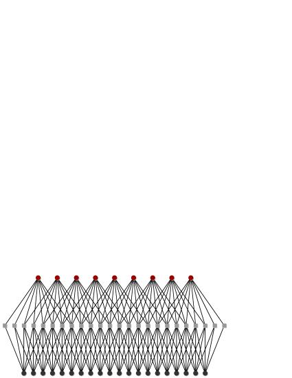
Figure 3: Protograph of $(8,4,5,4)$ SC-MN codes. Red variable nodes are punctured. Black variable nodes are transmitted.

In the protograph of $({\mathtt{l}},{\mathtt{r}},{\mathtt{g}},L)$ SC-MN codes, there are $V_{\mathrm{p}}=\hat{L}$ punctured variable nodes $V_{\mathrm{t}}={\mathtt{k}}\hat{L}+{\mathtt{l}}-{\mathtt{g}}+1$ unpunctured variable nodes, and $C={\mathtt{k}}\hat{L}+{\mathtt{l}}-2$ check nodes. Hence, in the limit of large $L$, the design coding rate is given as

$$R^{\mathrm{MN}}({\mathtt{l}},{\mathtt{r}},{\mathtt{g}},L)=\frac{V_{\mathrm{p}}+V_{\mathrm{t}}-C}{V_{\mathrm{t}}}$$

$$=\frac{\hat{L}+({\mathtt{k}}\hat{L}+{\mathtt{l}}-{\mathtt{g}}+1)-({\mathtt{k}}\hat{L}+{\mathtt{l}}-2)}{{\mathtt{k}}\hat{L}-{\mathtt{g}}+1}$$

$$=\frac{\hat{L}-{\mathtt{g}}+3}{{\mathtt{k}}\hat{L}-{\mathtt{g}}+1}=\frac{1}{{\mathtt{k}}}\quad(\hat{L}\to\infty).$$ (6)

The density is given by

$$d^{\mathrm{MN}}({\mathtt{l}},{\mathtt{r}},{\mathtt{g}},L) =\frac{{\mathtt{l}}V_{\mathrm{p}}+{\mathtt{g}}V_{\mathrm{t}}}{R^{\mathrm{MN}}({\mathtt{l}},{\mathtt{r}},{\mathtt{g}},L)V_{\mathrm{t}}}$$

$$={\mathtt{l}}+{\mathtt{g}}{\mathtt{k}}\quad(\hat{L}\to\infty).$$

The minimum density $4{\mathtt{k}}=4/R^{\mathrm{MN}}({\mathtt{l}},2,2,\infty)$ is attained when ${\mathtt{r}}={\mathtt{g}}=2$ and $L=\infty$.

Table 3 shows the BP threshold values and rates of $(4,2,2,L)$ SC-MN codes. As increasing $L$, it is observed that $\epsilon_{\mathrm{BP}}^{\mathrm{MN}}(4,2,2,L)$ approaches a value close to 1/2. From Eq. (6), it holds that $R^{\mathrm{MN}}(4,2,2,\infty)=1/2.$ This observation supports that threshold saturation occurs by SC-MN codes.

Table 3: BP threshold values and design coding rate of $(4,2,2,L)$ SC-MN codes. From Eq. (6), it holds that $R^{\mathrm{MN}}(4,2,2,\infty)=1/2.$

$L$	$\epsilon_{\mathrm{BP}}^{\mathrm{MN}}(4,2,2,L)$	$R^{\mathrm{MN}}(4,2,2,L)$
2	0.561146	0.363636
4	0.511397	0.421053
8	0.500252	0.457143
16	0.499977	0.477612
32	0.499908	0.488550

4.2 Spatially-Coupled Hsu-Anastasopoulos Codes

In this section, we propose spatial coupling of HA codes and evaluate the BP threshold values. An $({\mathtt{l}},{\mathtt{r}},{\mathtt{g}},L)$ SC-HA code is defined as a protograph code which is defined by base matrix

$$\begin{pmatrix}H({\mathtt{l}},{\mathtt{r}},\hat{L},{\mathtt{k}})&O\\ S({\mathtt{g}},{\mathtt{k}}\hat{L})&I\end{pmatrix}$$

and such that the bits corresponding to the left sub-matrix are punctured. Figure 4 shows the protograph $(4,8,5,9)$ SC-HA codes.

We assume that $\frac{{\mathtt{r}}}{{\mathtt{l}}}=:{\mathtt{k}}\in\mathbb{Z}.$ The protograph of the $({\mathtt{l}},{\mathtt{r}},{\mathtt{g}},L)$ SC-HA codes has $V_{\mathrm{p}}={\mathtt{k}}\hat{L}$ punctured information bit node, $V_{\mathrm{t}}=({\mathtt{k}}\hat{L}+{\mathtt{g}}-1)$ unpunctured bit nodes, and $C=(\hat{L}+{\mathtt{l}}-1)+({\mathtt{k}}\hat{L}+{\mathtt{g}}-1)$ check nodes. The design coding rate is given by

$$R^{\mathrm{HA}}({\mathtt{l}},{\mathtt{r}},{\mathtt{g}},L)=\frac{V_{\mathrm{p}}+V_{\mathrm{t}}-C}{V_{\mathrm{t}}}$$

$$\quad=\frac{({\mathtt{k}}-1)\hat{L}-{\mathtt{l}}+1}{{\mathtt{k}}\hat{L}+{\mathtt{g}}-1}=\frac{{\mathtt{k}}-1}{{\mathtt{k}}}\quad(\hat{L}\to\infty).$$ (7)

The density is given by

$$d^{\mathrm{HA}}({\mathtt{l}},{\mathtt{r}},{\mathtt{g}},L) =\frac{({\mathtt{l}}+{\mathtt{g}})V_{\mathrm{p}}+V_{\mathrm{t}}}{R^{\mathrm{HA}}({\mathtt{l}},{\mathtt{r}},{\mathtt{g}},L)V_{\mathrm{t}}}$$

$$=\frac{{\mathtt{k}}}{{\mathtt{k}}-1}(1+{\mathtt{g}}+{\mathtt{l}})\quad(\hat{L}\to\infty).$$

The minimum density $\frac{5{\mathtt{k}}}{{\mathtt{k}}-1}=5/R^{\mathrm{HA}}(2,{\mathtt{r}},2,\infty)$ is attained when ${\mathtt{l}}={\mathtt{g}}=2$ and $L=\infty$.

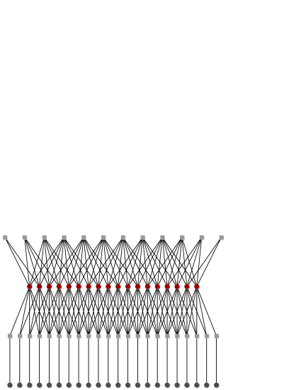
Figure 4: Protograph of $(8,4,5,9)$ SC-HA codes. Red variable nodes are punctured. Black variable nodes are transmitted.

Table 4 shows the BP threshold values of $(2,4,2,\hat{L})$ SC-HA code and design coding rates. As increasing $L$, it is observed that $\epsilon_{\mathrm{BP}}(2,4,2,L)$ approach a value close to 1/2. From Eq. (7), it holds that $R^{\mathrm{HA}}(2,4,2,\infty)=1/2.$ This observation supports that threshold saturation occurs by SC-HA codes.

Table 4: BP threshold values and design coding rate of $(2,4,2,L)$ SC-HA codes. From Eq. (7), it holds that $R^{\mathrm{HA}}(2,4,2,\infty)=1/2.$

$\hat{L}$	$\epsilon_{\mathrm{BP}}^{\mathrm{HA}}(2,4,2,L)$	$R^{\mathrm{HA}}(2,4,2,L)$
1	0.695420	0.285714
2	0.594441	0.363636
4	0.516970	0.421053
8	0.500460	0.457143
16	0.499980	0.477612
32	0.499909	0.488550

Discussion: We have proposed spatial-coupling of MN codes and HA codes. It is observed that the BP threshold values for BEC are very close to the Shannon limit. In other words, threshold saturation occurs for SC-MN codes and SC-HA codes. We observed such threshold saturation for various parameters with ${\mathtt{l}},{\mathtt{r}},{\mathtt{g}}\geq 2$. However, these BP threshold values leave a small gap to the Shannon limit. Such a gap was also observed when evaluating the BP threshold of the SC-LDPC codes [3]. Kudekar et al. proved that this is explained by wiggles appearing in EBP EXIT curves [3]. In order to decrease the gap, they introduced randomized SC-LDPC codes $({\mathtt{l}},{\mathtt{r}},L,w)$ that allow connections of edges with window size $w$. We observed the same effect on wiggles at the EBP EXIT curve of SC-MN codes. We will discuss the above observation in the next section.

5 Randomized Spatially-Coupled MacKay-Neal Codes

Figure 5: (a): The EBP EXIT curve of the $(4,2,2,L,w=2)$ SC-MN code ensemble.
(b): A closer look of the EBP EXIT curve of the $(4,2,2,L,w)$ SC-MN code ensemble.

In this section, we consider randomized SC-MN codes. Randomized SC-HA codes can be considered in a similar way. For simplicity, we focus only on randomized SC-MN codes.

We define an $({\mathtt{l}},{\mathtt{r}},{\mathtt{g}},L,w)$ SC-MN code ensemble as follows. The Tanner graph of a code in the $({\mathtt{l}},{\mathtt{r}},{\mathtt{g}},L,w)$ SC-MN code ensemble is constructed as follows. At each section $i\in\mathbf{Z}:=\{\dotsc,-2,-1,0,1,2,\dotsc\}$, consider $\frac{{\mathtt{r}}}{{\mathtt{l}}}M$ information nodes of degree ${\mathtt{l}}$, $M$ parity nodes of degree ${\mathtt{g}}$, and $M$ check nodes which has ${\mathtt{r}}$ incident information nodes and ${\mathtt{g}}$ parity nodes. Connect randomly these nodes in such a way that for $i\in\mathbf{Z}$ and $j=0,\dotsc,w-1$, information nodes at section $i$ and check nodes at section $i+j$ are connected with $\frac{{\mathtt{r}}M}{w}$ edges and parity nodes at section $i$ and check nodes at section $i+j$ are connected with $\frac{{\mathtt{g}}M}{w}$ edges. Shorten the information and parity bits at section $|i|>L$, i.e., set the bits to zero and do not transmit them. Puncture the information nodes at section $|i|\leq L$, i.e., the bits are not transmitted. Note that this ensemble is nicely represented by joint degree distributions [25]. The definition of the $({\mathtt{l}},{\mathtt{r}},{\mathtt{g}},L,w)$ SC-MN code ensemble is based on that of $({\mathtt{l}},{\mathtt{r}},L,w)$ randomized SC-LDPC code ensemble. For more details on $({\mathtt{l}},{\mathtt{r}},L,w)$ randomized SC-LDPC code ensemble, we refer the readers to [3, Section II.B].

Denote the number of transmitted bit nodes, punctured bit nodes by $V_{\mathrm{t}}$, $V_{\mathrm{p}}$, respectively.

$$V_{\mathrm{t}} =\hat{L}M,\quad V_{\mathrm{p}}=\frac{{\mathtt{r}}}{{\mathtt{l}}}\hat{L}M.$$

The number of check nodes of degree at least 1, denoted by $C$, can be counted by the same way as in [3, Lemma 3] as follows.

$$C =M[2L-w+2\sum_{i=0}^{w}(1-(\frac{i}{w})^{\mathtt{r}}(\frac{i}{w})^{{\mathtt{g}}})].$$

The design coding rate $R^{\mathrm{MN}}({\mathtt{l}},{\mathtt{r}},L,w)$ is given by

$$R^{\mathrm{MN}}({\mathtt{l}},{\mathtt{r}},L,w):=\frac{V_{\mathrm{t}}+V_{\mathrm{p}}-C}{V_{\mathrm{t}}}$$

$$=\frac{{\mathtt{r}}}{{\mathtt{l}}}+\frac{1+w-2\sum_{i=0}^{w}(1-(\frac{i}{w})^{\mathtt{r}}(\frac{i}{w})^{{\mathtt{g}}})}{\hat{L}}=\frac{{\mathtt{r}}}{{\mathtt{l}}}\quad(\hat{L}\to\infty).$$

Let $x_{i}^{(\ell)}$ and $y_{i}^{(\ell)}$ be the erasure probability of messages emitting from information-bit and parity-bit nodes, respectively, at section $i$ at the $\ell$-th round of BP decoding in the limit of large $M$. DE update equations of the randomized $({\mathtt{l}},{\mathtt{r}},{\mathtt{g}},L,w)$ SC-MN code are given as follows. For $|i|>L$, $x_{i}^{(\ell)}=y_{i}^{(\ell)}=0$ for $\ell\geq 0$. For $|i|\leq L$, $x_{i}^{(0)}=y_{i}^{(0)}=1$ for $\ell\geq 0$. For $|i|\leq L$,

$$x_{i}^{(\ell+1)}=$$

$$(\frac{1}{w}\sum_{j=0}^{w-1}[1-(1-\frac{1}{w}\sum_{k=0}^{w-1}x_{{i+j}-k}^{(\ell)})^{{\mathtt{r}}-1}(1-\frac{1}{w}\sum_{k=0}^{w-1}y_{{i+j}-k}^{(\ell)})^{{\mathtt{g}}}])^{{\mathtt{l}}-1}$$

$$y_{i}^{(\ell+1)}=$$

$$\epsilon(\frac{1}{w}\sum_{j=0}^{w-1}[1-(1-\frac{1}{w}\sum_{k=0}^{w-1}x_{{i+j}-k}^{(\ell)})^{{\mathtt{r}}}(1-\frac{1}{w}\sum_{k=0}^{w-1}y_{{i+j}-k}^{(\ell)})^{{\mathtt{g}}-1}])^{{\mathtt{g}}-1}$$

Consider fixed points of the DE system, i.e., $(\underline{x}:=(x_{-L},\dotsc,x_{L}),\underline{y}:=(y_{-L},\dotsc,y_{L}),\epsilon)$ such that $x_{i}=y_{i}=0$ for $|i|>L,$ and

$$x_{i}= \bigl{(}\frac{1}{w}\sum_{j=0}^{w-1}[1-(1-\frac{1}{w}\sum_{k=0}^{w-1}x_{{i+j}-k})^{{\mathtt{r}}-1}(1-\frac{1}{w}\sum_{k=0}^{w-1}y_{{i+j}-k})^{{\mathtt{g}}}]\bigr{)}^{{\mathtt{l}}-1}$$

$$y_{i}= \epsilon\bigl{(}\frac{1}{w}\sum_{j=0}^{w-1}[1-(1-\frac{1}{w}\sum_{k=0}^{w-1}x_{{i+j}-k})^{{\mathtt{r}}}(1-\frac{1}{w}\sum_{k=0}^{w-1}y_{{i+j}-k})^{{\mathtt{g}}-1}]\bigr{)}^{{\mathtt{g}}-1}$$

For any $\epsilon\in[0,1]$, a fixed point $(\epsilon,\underline{x}=\underline{0},\underline{y}=\underline{0})$ is called trivial. Trivial fixed points is corresponds to the message density $(\underline{x},\underline{y})=(\underline{0},\underline{0})$ of successful decoding. The EBP EXIT curve is defined as the projected plots $(\epsilon,h^{\mathrm{EBP}}(\epsilon))$ of fixed points $(\epsilon,\underline{x},\underline{y})$, other than trivial ones, onto the following EXIT function.

$$h^{\mathrm{EBP}}(\epsilon)= \frac{1}{\hat{L}}\sum_{i=-L}^{L}(\frac{1}{w}\sum_{j=0}^{w-1}[1-(1-\frac{1}{w}\sum_{k=0}^{w-1}x_{{i+j}-k})^{{\mathtt{r}}}$$

$$\cdot(1-\frac{1}{w}\sum_{k=0}^{w-1}y_{{i+j}-k})^{{\mathtt{g}}-1}])^{{\mathtt{g}}}.$$

Figure 5 (a) plots the EBP EXIT curve of the $(4,2,2,L,w=2)$ SC-MN code ensemble. Consider no points of the EBP curve $(\epsilon,h^{\mathrm{EBP}}(\epsilon))$ are at $\epsilon\in[0,\epsilon^{\prime}]$. This suggests that there are only trivial fixed points of DE with $\epsilon\in[0,\epsilon^{\prime}]$ and $(\underline{x}^{(\ell)},\underline{y}^{(\ell)})$ converges to the trivial fixed point. It follows that the BP threshold $\epsilon_{\mathrm{BP}}^{\mathrm{MN}}({\mathtt{l}},{\mathtt{r}},{\mathtt{g}},L,w)$ is given by $\epsilon$ at which the left-most cliff edge of the curve vertically drops [3]. The BP threshold in Fig. 5 (a) is very close to 1/2. However, there exists a small gap. A closer look at the cliff edge of the green curve given in Fig. 5 (b) reveals the cliff of $(4,2,2,L=32,w=2)$ SC-MN codes have wiggles. The wiggle size decreases by increasing $w$ as seen in Fig. 5 (b).

Figure 6 and 7 plot the EBP EXIT curves $(\epsilon,h^{\mathrm{EBP}})$ and $(y_{i},h^{\mathrm{EBP}})$ of the $(4,2,3,16,w)$ SC-MN code ensemble for $w=2$ and $w=4$, respectively. It is observed that as decreasing $h^{\mathrm{EBP}}$ value, $y_{i}$ starts to collapse from the boundaries $|i|=L$ and gradually to the center $i=0$. It is observed that uncollapsed $y_{i}$ takes almost the same value $0.5$. Each time $y_{i}$ collapse, $\epsilon$ is affected a little, which gives rise to a wiggle. By increasing $w$, each $y_{i}$ collapses slowly, which gives rise to a smaller wiggle.

Figure 6: The EBP EXIT curve $(\epsilon,h^{\mathrm{EBP}})$ and $(y_{i},h^{\mathrm{EBP}})$ of the $(4,2,3,L=16,w=2)$ SC-MN code ensemble.

Figure 7: The EBP EXIT curve $(\epsilon,h^{\mathrm{EBP}})$ and $(y_{i},h^{\mathrm{EBP}})$ of the $(4,2,3,L=16,w=4)$ SC-MN code ensemble.

6 Conclusion

We have proposed spatial-coupling of MN (resp. HA) codes with bounded density. By DE analysis, we observed that the BP threshold values of the SC-MN (resp. SC-HA) codes for BEC are very close to the Shannon limit. This empirical evidence supports that the SC-MN (resp. SC-HA) codes may achieve the Shannon limit of the BEC. In other words, threshold saturation occurs for SC-MN codes and SC-HA codes. We observed such threshold saturation for various parameters with ${\mathtt{l}},{\mathtt{r}},{\mathtt{g}}\geq 2$.

We further investigate the EBP EXIT curve of randomized SC-MN codes. We observed that the small gap between BP threshold and the Shannon limit is caused by wiggles of BP EXIT curve. By increasing the randomized window size $w$, the wiggle size largely decreased.

References

- [1] T. Richardson and R. Urbanke, Modern Coding Theory, Cambridge University Press, March 2008.
- [2] E. Arıkan, “Channel polarization: A method for constructing capacity-achieving codes for symmetric binary-input memoryless channels,” IEEE Trans. Inf. Theory, vol.55, no.7, pp.3051–3073, July 2009.
- [3] S. Kudekar, T. Richardson, and R. Urbanke, “Threshold saturation via spatial coupling: Why convolutional LDPC ensembles perform so well over the BEC,” IEEE Trans. Inf. Theory, vol.57, no.2, pp.803–834, Feb. 2011.
- [4] S. Kudekar, C. Méasson, T.J. Richardson, and R.L. Urbanke, “Threshold saturation on BMS channels via spatial coupling,” http://arxiv.org/abs/1004.3742, April 2010.
- [5] A.J. Felström and K.S. Zigangirov, “Time-varying periodic convolutional codes with low-density parity-check matrix,” IEEE Trans. Inf. Theory, vol.45, no.6, pp.2181–2191, June 1999.
- [6] M. Lentmaier, D.V. Truhachev, and K.S. Zigangirov, “To the theory of low-density convolutional codes. II,” Probl. Inf. Transm. , no.4, pp.288–306, 2001.
- [7] A. Sridharan, J. M. Lentmaier, D. J. Costello, and K.S. Zigangirov, “Convergence analysis of a class of LDPC convolutional codes for the erasure channel,” Proc. 42th Annual Allerton Conf. on Commun., Control and Computing, Montecillo, Illinois, USA, Oct. 2004.
- [8] M. Lentmaier, A. Sridharan, D.J. Costello, Jr., and K.S. Zigangirov, “Iterative decoding threshold analysis for LDPC convolutional codes,” IEEE Trans. Inf. Theory, vol.56, no.10, pp.5274 –5289, Oct. 2010.
- [9] C. Méasson, A. Montanari, T. Richardson, and R. Urbanke, “The generalized area theorem and some of its consequences,” IEEE Trans. Inf. Theory, vol.55, no.11, pp.4793 –4821, Nov. 2009.
- [10] G. Miller and D. Burshtein, “Bounds on the maximum-likelihood decoding error probability of low-density parity-check codes,” IEEE Trans. Inf. Theory, vol.47, no.7, pp.2696–2710, Nov. 2001.
- [11] T.J. Richardson, M.A. Shokrollahi, and R.L. Urbanke, “Design of capacity-approaching irregular low-density parity-check codes,” IEEE Trans. Inf. Theory, vol.47, no.2, pp.619–637, Feb. 2001.
- [12] R. Mori and T. Tanaka, “Performance and construction of polar codes on symmetric binary-input memoryless channels,” http://arxiv.org/abs/0901.2207, Jan. 2009.
- [13] A. Khandekar and R. McEliece, “On the complexity of reliable communication on the erasure channel,” Proc. 2001 IEEE Int. Symp. Inf. Theory (ISIT), p.1, June 2001.
- [14] D. Mitchell, M. Lentmaier, and D. Costello, “New families of ldpc block codes formed by terminating irregular protograph-based LDPC convolutional codes,” Proc. 2010 IEEE Int. Symp. Inf. Theory (ISIT), pp.824 –828, June 2010.
- [15] I. Sason and R. Urbanke, “Parity-check density versus performance of binary linear block codes over memoryless symmetric channels,” IEEE Trans. Inf. Theory, vol.49, no.7, pp.1611 – 1635, July 2003.
- [16] T. Richardson and R. Urbanke, “Multi-edge type LDPC codes,” 2003. preprint available at http://citeseerx.ist.psu.edu/viewdoc/summary?doi=10.1.1.106.7310.
- [17] H. Pfister and I. Sason, “Accumulate repeat accumulate codes: Capacity-achieving ensembles of systematic codes for the erasure channel with bounded complexity,” IEEE Trans. Inf. Theory, vol.53, no.6, pp.2088 –2115, June 2007.
- [18] D. MacKay, “Good error-correcting codes based on very sparse matrices,” IEEE Trans. Inf. Theory, vol.45, no.2, pp.399 –431, March 1999.
- [19] T. Murayama, Y. Kabashima, D. Saad, and R. Vicente, “Statistical physics of regular low-density parity-check error-correcting codes,” Phys. Rev. E, vol.62, no.2, pp.1577–1591, Aug. 2000.
- [20] T. Tanaka and D. Saad, “Typical performance of regular low-density parity-check codes over general symmetric channels,” J. Phys. A: Math. Gen. , vol.36, no.43, pp.11143–11157, Oct. 2003.
- [21] C.H. Hsu and A. Anastasopoulos, “Capacity-achieving codes with bounded graphical complexity and maximum likelihood decoding,” IEEE Trans. Inf. Theory, vol.56, no.3, pp.992 –1006, March 2010.
- [22] J. Cheng and R. McEliece, “Some high-rate near capacity codecs for the gaussian channel,” Proc. 34th Annual Allerton Conf. on Commun., Control and Computing, Oct. 1996.
- [23] M. Wainwright and E. Martinian, “Low-density graph codes that are optimal for binning and coding with side information,” IEEE Trans. Inf. Theory, vol.55, no.3, pp.1061 –1079, March 2009.
- [24] J. Thorpe, “Low-density parity-check (LDPC) codes constructed from protographs,” IPN Progress Report, pp.42–154, Aug. 2003.
- [25] K. Kasai, T. Shibuya, and K. Sakaniwa, “Detailedly represented irregular low-density parity-check codes,” IEICE Trans. Fundamentals, vol.E86-A, no.10, pp.2435–2444, Oct. 2003.