Abstract

According to recent results, the Gell-Mann – Low function $\beta(g)$ of four-dimensional $\phi^{4}$ theory is non-alternating and has a linear asymptotics at infinity. According to the Bogoliubov and Shirkov classification, it means possibility to construct the continuous theory with finite interaction at large distances. This conclusion is in visible contradiction with the lattice results indicating triviality of $\phi^{4}$ theory. This contradiction is resolved by a special character of renormalizability in $\phi^{4}$ theory: to obtain the continuous renormalized theory, there is no need to eliminate a lattice from the bare theory. In fact, such kind of renormalizability is not accidental and can be understood in the framework of Wilson’s many-parameter renormalization group. Application of these ideas to QCD shows that Wilson’s theory of confinement is not purely illustrative, but has a direct relation to a real situation. As a result, the problem of analytical proof of confinement and a mass gap can be considered as solved, at least on the physical level of rigor.

Introduction

Recent investigations of the strong coupling regime in $\phi^{4}$ theory revealed unexpected feature in its renormalizability: the continual limit in the renormalized theory does not require the continual limit in the bare theory. We show below that such kind of renormalizability has a general character and can be understood in the framework of Wilson’s many-parameter renormalization group. These results allow to give a final solution to the problem of triviality or non-triviality of $\phi^{4}$ theory. Application of these ideas to the Wilson theory of confinement shows that this theory is not purely illustrative, but has a direct relation to real QCD. As a result, the problem of analytical proof of confinement and a mass gap can be considered as solved, at least on the physical level of rigor.

1. Triviality

According to recent results [1, 2, 3, 4] (see also [5, 6]), the Gell-Mann – Low function $\beta(g)$ in four-dimensional $\phi^{4}$ theory is non-alternating and has asymptotic behavior $\beta(g)=4g$ at $g\to\infty$. According to the Bogoliubov and Shirkov classification [7] (see discussion in [3]), it means possibility to construct the continuous theory with finite interaction at large distances. This conclusion is in visible contradiction with lattice results indicating triviality of $\phi^{4}$ theory (see [8]–[12] and numerous references in [13]).

In fact, one should differ two definitions of triviality. According to Wilson [8], triviality means that integration of the Gell-Mann – Low equation

$$-\frac{dg}{d\ln L}=\beta(g)$$

in the direction of large distances $L$ gives the effective charge $g$ tending to zero (Fig.1,a); this definition implies the massless theory, since in the opposite case the distance scale is saturated by the inverse mass. The definition of true triviality is different (Fig.1,b).

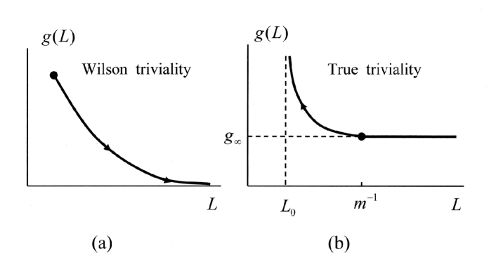
Figure 1: Wilson triviality (a) against true triviality (b).

In this case one considers the massive theory and suggests the finite interaction $g_{\infty}$ for $L\mathbin{\lower 3.0pt\hbox{$\hbox to0.0pt{\raise 5.0pt\hbox{$\char 62\relax$}\hss}\mathchar 29208\relax$}}m^{-1}$; a theory is trivial, if integration of the Gell-Mann – Low equation in the direction of small $L$ gives a divergency at finite $L_{0}$ (the so called Landau pole) and does not allow to reach the $L\to 0$ limit. Such situation is internally inconsistent [7] and means incorrectness of the initial suggestion on finite interaction at large distances; in fact, $L_{0}\to 0$ if $g_{\infty}\to 0$. Wilson triviality means that $\beta$-function is non-negative and has a zero only for $g=0$. True triviality needs in addition its sufficiently quick growth at infinity, $\beta(g)\sim g^{\alpha}$ with $\alpha>1$. According to [1]–[6], $\phi^{4}$ theory and QED are trivial in the Wilson sense, but do not possess true triviality.

Two definitions of triviality were hopelessly mixed in literature [13]. The reasons for it are as follows:

(a) Bogoliubov and Shirkov’s work is poorly known to Western community;

(b) It is rather difficult to test true triviality in the lattice approach ;

(c) There exist arguments that ”prove” equivalence of two definitions.

As illustration to the latter point, consider the following reasoning. The only alternative to perturbative approach is to express all quantities related to renormalized theory in terms of the functional integrals. The latter depend on the bare charge $g_{0}$, bare mass $m_{0}$ and the ultraviolet cut-off $\Lambda$. Taking into account their dimensional character, one has the following relations for the renormalized charge $g$, renormalized mass $m$ and observable quantities $A_{i}$

$$g=F_{g}\left(g_{0},m_{0}/\Lambda\right)\,,\qquad$$

$$m=\Lambda F_{m}\left(g_{0},m_{0}/\Lambda\right)\,,\qquad$$

$$A_{i}=\Lambda^{d_{i}}F_{i}\left(g_{0},m_{0}/\Lambda\right)\,,\qquad$$

where $d_{i}$ is a physical dimensionality of $A_{i}$. Excluding $g_{0}$ and $m_{0}/\Lambda$ in favor of $g$ and $m/\Lambda$, one has

$$A_{i}=m^{d_{i}}\tilde{F}_{i}\left(g,m/\Lambda\right)\,.\qquad$$

To eliminate the dependence on $\Lambda$ we should take the limit $m/\Lambda\to 0$. In the lattice approach, this limit corresponds to $\xi/a\to\infty$ ($\xi$ is a correlation length and $a$ is a lattice spacing), i.e. to the phase transition point. The latter is determined by a zero of $\beta$-function, which gives $g=0$ in four-dimensional $\phi^{4}$ theory.

In this argumentation, Wilson triviality was considered as given, while true triviality was ”derived” from it. Of course, it cannot be correct, because two definitions are surely not equivalent. This shortcoming originates from our assumption that a general-position situation takes place in Eq. 4: in this case we indeed should take a limit $m/\Lambda\to 0$. This limit is unnecessary, if dependence on $m/\Lambda$ is absent in Eq. 4. Such special case fills the ”gap” between two definitions and makes them not equivalent.

Such special case really holds in $\phi^{4}$ theory [3, 4]. Let us return to Eqs. 3 and impose the condition $m\ll\Lambda$, corresponding to the continuum limit of the renormalized theory. If this condition is imposed in the region $g_{0}\gg 1$, then $\phi^{4}$ theory reduces to the Ising model, containing the single parameter $\kappa$, which plays the role of inverse temperature [3, 4]; relations (3) accept the form

$$g=F_{g}\left(\kappa\right)\,,\qquad$$

$$m=\Lambda F_{m}\left(\kappa\right)\,,\qquad$$

$$A_{i}=\Lambda^{d_{i}}F_{i}\left(\kappa\right)\,.\qquad$$

So far there is nothing unusual: the condition $m/\Lambda\to 0$ gives a relation between $g_{0}$ and $m_{0}/\Lambda$, so all functions in Eq.3 depend on the single parameter, which we denoted as $\kappa$. The non-trivial point consists in the following: the condition $m/\Lambda\ll 1$ is sufficient for transformation to the Ising model, but not necessary for it. In fact, such transformation is possible under the weaker conditions, which are compatible with the arbitrary value of $m/\Lambda$ [3, 4]. Excluding $\kappa$ from (5), one obtains the equations

$$A_{i}=m^{d_{i}}F_{i}\left(g\right)\,,\qquad$$

which are analogous to (4), but do not contain the parameter $m/\Lambda$. As a result, the program of renormalization is completely fulfilled, and no additional limiting transitions are necessary. It means that (a) we can retain the lattice in the bare theory (as a convenient tool for representation of functional integrals), and (b) relation between $m$ and $\Lambda$ (or $\xi$ and $a$) can be arbitrary, so the arbitrary value of $g$ becomes possible.

Usually, the lattice theory contains more parameters than the initial field theory. For example, discretization of the gradient term in $d$-dimensional $\phi^{4}$ theory

$$\int d^{d}x\left[\nabla\phi(x)\right]^{2}=-\int d^{d}x\phi(x)\nabla^{2}\phi(x)\quad\longrightarrow\quad\sum_{x,x^{\prime}}J_{x-x^{\prime}}\phi_{x}\phi_{x^{\prime}}\,,$$

corresponds to the replacement of $-\nabla^{2}=\hat{p}^{2}$ by $\epsilon({\hat{p}})$, where $\epsilon({p})$ is a bare lattice spectrum

$$\epsilon({p})=\sum_{x}J_{x}{\rm e}^{i{p\cdot x}}=p^{2}+O(p^{4})\,,$$

while ${\hat{p}}$ is the momentum operator and $\exp\{i{\hat{p}\cdot x}\}$ is the operator of shift on the vector ${x}$. The overlap integrals $J_{x}$ can be taken arbitrary and are restricted only by the condition (8). The interesting question arises: if we can retain a lattice in the bare theory, then what lattice model should be chosen?

A solution can be found from Eq. 4. Since dependence on $m/\Lambda$ is absent, we can take $m/\Lambda\to 0$. But in this limit (when $\xi/a\to\infty$) there are physical grounds for independence of functions $F_{i}$ on the way of cut-off. If such independence takes place for $m/\Lambda\to 0$, it retains for arbitrary $m/\Lambda$ due to independence of functions $F_{i}$ on this parameter. In fact, this argumentation implies renormalizability of theory (due to which the dependence on $\Lambda$ can be excluded) and belonging of the lattice model to the proper universality class (inside of which the dependence on the way of cut-off is absent).

The lattice theory is frequently considered as a reasonable approximation to the true field theory. In this case we should accept the condition $\xi\gg a$, which signifies that one has a lot of lattice sites on the characteristic scale of variation of field. This condition can be strengthen till $\xi/a\to\infty$ or liberalized till $\xi\mathbin{\lower 3.0pt\hbox{$\hbox to0.0pt{\raise 5.0pt\hbox{$\char 62\relax$}\hss}\mathchar 29208\relax$}}a$. The first case corresponds to the point of phase transition and gives $g=0$. In the second case we obtain restriction $g\mathbin{\lower 3.0pt\hbox{$\hbox to0.0pt{\raise 5.0pt\hbox{$\char 60\relax$}\hss}\mathchar 29208\relax$}}1$ (for the proper charge normalization [4]), which can be used to obtain the upper bound on the Higgs mass [12, 14].

In fact, the lattice theory should not be considered as any approximation to field theory, though it is possible for $g_{0}\ll 1$. The true field theory is continuous from the very beginning and does not contain any lattice. The lattice is present only in the bare theory, which is an auxiliary construction and is completely removed later. No physical requirements, like $\xi\gg a$, are relevant for it. If one removes the condition $\xi\gg a$, then any values of $g$ become admissible . In fact, a real designation of the bare theory is to represent the relations between physical quantities in the parametric form (3). Such representation has no deep sense already due to its ambiguity: it can be written in many different forms, changing $g_{0}$ and $m_{0}/\Lambda$ by any other pair of variables.

We see that contradiction between the continual and lattice approaches is resolved by a special character of renormalizability in $\phi^{4}$ theory:

Correct relations (6) between physical quantities can be obtained for the arbitrary value of the parameter $a/\xi$, while the dependence on this parameter is absent. To obtain the continuous renormalized theory, there is no need to eliminate a lattice from the bare theory.

2. Renormalizability

The interesting question arises: Is such kind of renormalizability related with the specific properties of $\phi^{4}$ theory, or it is a manifestation of some general mechanism?

We shall see below that the second variant is correct. It can be understood in the framework of Wilson’s many-parameter renormalization group (RG) [8]. According to it, the parameters $p_{i}$ of some lattice Hamiltonian are considered as functions of the length scale ${\it l}$.  The flow of these parameters is determined by the RG equations, which can be written in the differential form

$$-\frac{dp_{i}}{d\ln({\it l}/a)}=F_{i}\{p_{k}\}\,.$$

These equations can be linearized near the fixed point

$$p_{i}({\it l})=p^{*}_{i}\qquad\mbox{ (\,for\quad all\quad{\it l\,})}$$

and investigated by the standard methods of linear algebra. The ordinary phase transitions are described by the saddle points of such equations. The simplest saddle point in two parameter space (Fig.2) has the straight-line trajectories in

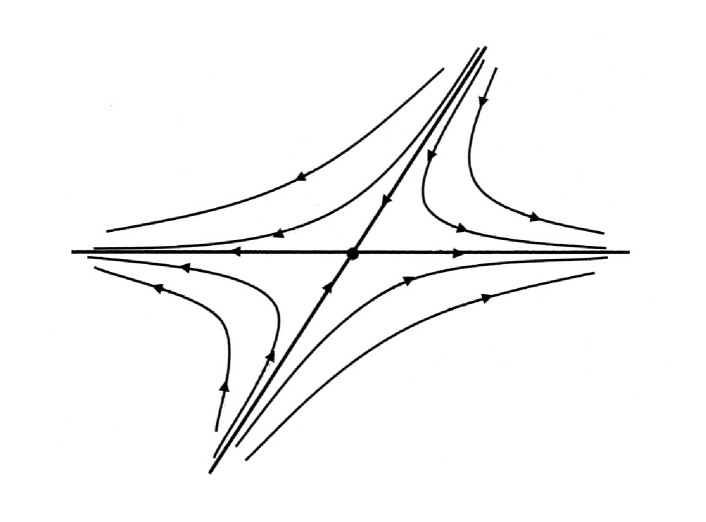
Figure 2: Simplest variant of the saddle point.

two main directions (one stable and one unstable), while the rest of trajectories are hyperbolic. For the usual phase transitions, there are infinite number of stable directions and one (in the simplest case) unstable direction. The latter is related with some controlling parameter like temperature, measuring the distance to the critical point.

Instead of increasing ${\it l}$ for fixed $a$, we can diminish $a$ for fixed ${\it l}$. The continuum limit $a\to 0$ of field theory corresponds to the critical surface $\xi/a=\infty$ in the many-parameter space (Fig.3).

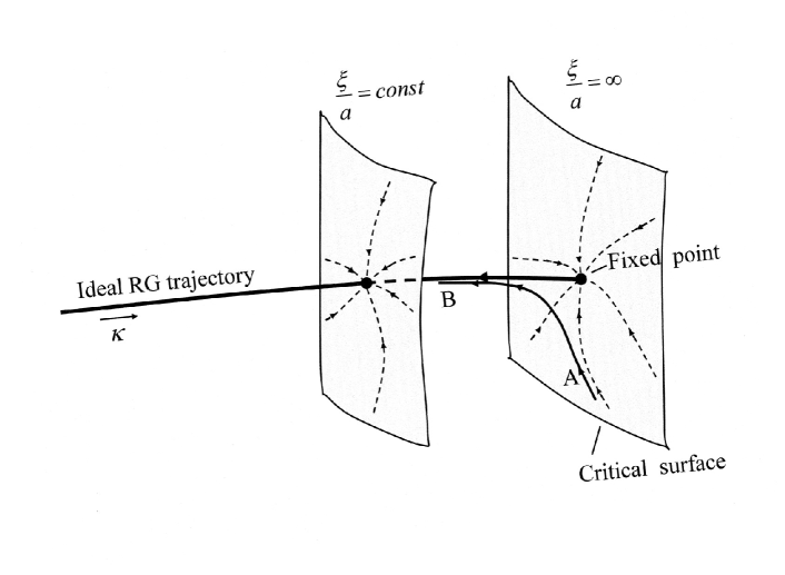
Figure 3: Schematic of the Wilson many-parameter space.

All trajectories at the critical surface tend to the fixed point. The unstable trajectory, originating in the fixed point will be referred as an ”ideal RG trajectory”: along it one has the exact one-parameter scaling, which is a pipe dream in many fields of physics (see e.g. [15]). To define it rigorously, let us consider the limit $a\to 0$ with fixed $\xi/a$; then all trajectories lying at the surface $\xi/a=const$ (Fig.3) tend to one point (analogously to the critical surface), while the locus of such points is the ideal RG trajectory.

Let the parameter $\kappa$ is measuring the distance along the ideal trajectory: then $\xi/a$ (or $\Lambda/m$) is a function of $\kappa$. Analogously, all dimensionless quantities depend only on $\kappa$, while the dimensional quantities are measured in units of $\Lambda$. As a result, we come to equations

$$g=F_{g}\left(\kappa\right)\,,\qquad m=\Lambda F_{m}\left(\kappa\right)\,,\qquad A_{i}=\Lambda^{d_{i}}F_{i}\left(\kappa\right)\,,$$

which coincide with (5) and give the relations (6) with no dependence on $m/\Lambda$.

The above construction has a following sense. If the limit $a\to 0$ is taken in the arbitrary manner, then the system will go to infinity along the unstable direction and appear far from the critical surface, which is our goal. Therefore, we suggest to take the continual limit in two steps:

(a) take a limit $a\to 0$ for $a/\xi=const$;

(b) take a limit $a/\xi\to 0$.

It appears, that the dependence on $a$ in renormalized theory disappears already at the first step. The second step becomes unnecessary and we need not take the continuum limit in the bare theory. The $const$ appearing in (a) is one of the possible definitions of the parameter $\kappa$.

These ideas are close to the QCD specialists, and in fact the above consideration was partially taken from ”Introduction to lattice QCD” by R. Gupta [16]. This picture is discussed there in relation to improvement of the lattice action, and the author claims that simulations, done along the ideal RG trajectory, will reproduce the continuum physics without discretization errors. It implies the absence of $a/\xi$ dependence, in accordance with our results. Only final conclusion was not made, that the continuum limit is not necessary in the bare theory. In fact, this conclusion goes across the present-day practice in lattice simulations, which are made in the region of large $\xi/a$ (typically $\xi/a=5\div 15$) with accurate extrapolation to $a/\xi\to 0$.

Any RG trajectory is a line of ”constant physics”, since the RG transformation is simply the mental construction, which does not affect the large-scale properties of the system. All trajectories belonging to the critical surface and meeting in the fixed point are physically equivalent, corresponding to the unique continuous field theory. The ideal RG trajectory originating in the fixed point gives the equivalent representation for field theory. Let us consider the trajectory $AB$, which begins near the critical surface and goes along it, and then tends to the ideal RG trajectory (Fig.3). Introducing $\tilde{\kappa}$ as a distance along $AB$, we come to the parametric representation analogous (11)

$$g=\tilde{F}_{g}\left(\tilde{\kappa}\right)\,,\qquad m=\Lambda\tilde{F}_{m}\left(\tilde{\kappa}\right)\,,\qquad A_{i}=\Lambda^{d_{i}}\tilde{F}_{i}\left(\tilde{\kappa}\right)\,,$$

and relations (6), independent of $\xi/a$. The choice of small or large $\xi/a$ values corresponds to the ”ends” of trajectory $AB$ which are arbitrary close to the critical surface and the ideal trajectory; hence, the obtained relations (6) correspond to continual theory. However, the parametric representation (12) is essentially different from (11) and is not reduced to the change of variables $\kappa=f(\tilde{\kappa})$. To understand it, let us retain definition of $\kappa$ as a distance along the ideal trajectory, and assign it to the point of $AB$, corresponding to the same value of $\xi/a$. Then the second relation (12) will be the same as (11), but the rest two relations remain different:

$$g=\tilde{F}_{g}\left(\kappa\right)\,,\qquad m=\Lambda F_{m}\left(\kappa\right)\,,\qquad A_{i}=\Lambda^{d_{i}}\tilde{F}_{i}\left(\kappa\right)\,.$$

Indeed, the charge $g$ usually belongs to irrelevant parameters and we can introduce ”the axis of charges” at the critical surface; the fixed point corresponds to $g=0$. If the limit $a/\xi\to 0$ is taken along the ideal trajectory, then $g\to 0$. If this limit is taken along $AB$, then the arbitrary function $g=\tilde{F}_{g}(\kappa)$ in $(12^{\prime})$ is possible: it depends on the direction of $AB$ relative to ”the axis of charges”. The functional relation between $g$ and $\kappa$ becomes indeterminate and can be omitted.

As a result, the renormalized and bare sectors of theory become decoupled. The renormalized sector contains relations (6), where $g$ and $m$ are considered as independent variables. The bare sector contains only relation $a/\xi=m/\Lambda=F_{m}\left(\kappa\right)$, which determines $\kappa$ as a function of $a$ and is irrelevant from viewpoint of physics. Parameter $a/\xi$ becomes absolutely free.

The set of different trajectories $AB$ defines the universality class of the corresponding field theory. Such trajectories fill the whole space, if the critical surface and the ideal RG trajectory are unbounded. In fact, the critical surface is certainly restricted in some directions, because there are a lot of such surfaces, corresponding to different phase transitions. To obtain the correct relations (6), there is no need to construct the ideal RG trajectory: it suffices to find the arbitrary trajectory like $AB$, belonging to the same universality class.

As a result, we come to the following conclusion:

Renormalizable theory of the considered type allows representation in the form of lattice theory, which gives the correct relations between physical quantities, and contains free parameter $a/\xi$, which does not enter these relations.

QCD with one sort of quarks contains two parameters, interaction constant $g$ and the quark mass $m$. Its renormalization properties are analogous to those of $\phi^{4}$ theory or QED and are expressed by the relations (3, 4); in fact Sec.2 set axiomatic for study of such theories. We restrict our discussion by a theory without quarks, i.e. pure Yang-Mills theory; then the quark mass is not included as a parameter and the theory does not contain any natural mass scale. To avoid the specific difficulties related with such situation, let us introduce the ”extended version” of Yang-Mills theory, where the role of the bare quark mass $m_{0}$ (more exactly, the ratio $m_{0}/\Lambda$) is played by some auxiliary parameter $p$ characterizing the lattice theory; as a renormalized mass, we accept the mass $m$ of the lightest glueball (the bound state of several gluons), while the correlation length $\xi$ is defined as $m^{-1}$. Thereby, two bare parameters $g_{0}$ and $p$ provide the observable values for renormalized $g$ and $m$ ($g$ corresponds to the momentum scale $m$). In order to return to the standard variant of theory, we should remove the introduced extra degree of freedom by fixing one relation between observable quantities. However, it can be done on the late stage (see the end of Sec.3), while the main of analysis is produced for the ”extended version”, which is analogous to $\phi^{4}$ theory.

According to Wilson [18], confinement can be proved in the lattice version of the Yang-Mills theory for large value of the bare charge $g_{0}$. The energy of interaction for two probe quarks, separated by a distance $R$, is $V(R)=\sigma R$, while the string tension $\sigma$ and the glueball mass $m$ are given by expressions [16, 18, 19]

$$\sigma=\frac{\ln(3g_{0}^{2})}{a^{2}}\,,\qquad m=\frac{4\,\ln(3g_{0}^{2})}{a}\,.$$

In spite of the evident success, the Wilson theory is considered as purely illustrative and having no relation to real QCD. As was indicated by Wilson himself, his theory corresponds to a situation

$$\xi\ll a\qquad\mbox{ or}\qquad m\gg\Lambda\,,$$

which is considered as unphysical. An attempt to advance into the physical region inevitably destroys the strong coupling regime. Indeed, fixing $\sigma$ to its observable value, we have $g^{2}_{0}(a)=(1/3)\exp\{\sigma a^{2}\}$ and substitution to the Gell-Mann – Low equation in the cut-off scheme [20]

$$-\frac{d\,g_{0}^{2}}{d\,\ln a^{2}}=\beta(g_{0}^{2})=\beta_{0}g_{0}^{4}+\beta_{1}g_{0}^{6}+\ldots$$

gives $\beta(g^{2}_{0})=-g_{0}^{2}\ln(3g_{0}^{2})$ for large $g_{0}$ [21]. Together with a negative sign of $\beta_{0}$ and $\beta_{1}$ it implies the negative $\beta$-function for all $g_{0}$ (Fig.4);

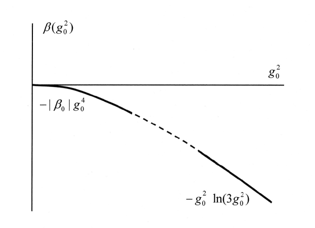
Figure 4: The Gell-Mann – Low function of the Yang-Mills theory in the cut-off scheme.

the lattice results confirm this conclusion (see also [22]). In this case $g_{0}$ tends to zero in the continuum limit $a\to 0$. It does not mean triviality of theory, because the behavior $g_{0}\to 0$ is compatible with a finite value of the renormalized charge $g$, as can be seen from the one-loop result for $\Lambda\to\infty$

$$g^{2}_{0}=\frac{g^{2}}{1+|\beta_{0}|g^{2}\ln\Lambda^{2}/m^{2}}\,\,\longrightarrow\,\,\frac{1}{|\beta_{0}|\ln\Lambda^{2}/m^{2}}\,\,\longrightarrow\,\,\,0\,\,.$$

Triviality is avoided, but the strong coupling regime is inevitably destroyed and Wilson’s theory becomes inapplicable.

The situation changes drastically, if we use representation (5, 6) introduced in the previous sections. In this case:

(1) We do not need to take the continual limit in the bare theory, so $g_{0}$ remains finite.

(2) Due to absence of the $\xi/a$ dependence, this parameter can be taken arbitrary: it eliminates objections against the non-physical regime in Wilson’s theory.

(3) Experience of $\phi^{4}$ theory shows that there is no direct relation between the bare and renormalized charge : representation (5) is rigorously introduced in the limit $g_{0}\to\infty$ (see Footnote 2), while $g$ remains to be a finite function of $\kappa$ [4]. With some reservations, the same property is valid in Yang-Mills theory. Rewriting the second expression (13) in the form

$$g_{0}^{2}=\frac{1}{3}\exp\left(\frac{ma}{4}\right)=\frac{1}{3}\exp\left\{\frac{a}{4\xi}\right\}\,,$$

we see that, independently of renormalized values of $g$ and $m$, it is possible to choose the free parameter $a/\xi$ so as to obtain the sufficiently large value for $g_{0}$. Then Wilson’s theory becomes applicable and the first relation (13) gives finite value for $\sigma$, i.e. confinement.

We have used the relations (13), which are valid for the simplest Wilson action [16, 18, 19]. However, the latter is not suitable for our purposes due to a trivial fact that it does not contain the sufficient number of parameters. To obtain the observable values of $\sigma$ and $m$

$$\sigma=a^{-2}f_{\sigma}(g_{0})\,,\qquad m=a^{-1}f_{m}(g_{0})\,,\qquad$$

one should fix both $g_{0}$ and $a$; but the fixed $a$ means that it is impossible to introduce representation with free parameter $a/\xi$. Therefore, we should consider some generalizations.

The simplest Wilson action [16, 18, 19]

$$S=-\frac{1}{g_{0}^{2}}\sum_{\Box}W_{\Box}^{1\times 1}$$

is a sum over all plaquettes $\Box$ of size $1\times 1$, where the plaquette contribution $W_{\Box}^{1\times 1}$ is determined by a product of matrices attributed to the sides of a plaquette. In the contemporary investigations, more complicated forms of the action are used which contain contributions of $m\times n$ plaquettes [16]

$$S=-\frac{1}{g_{0}^{2}}\sum_{\Box}\sum_{m,n}C_{mn}W_{\Box}^{m\times n}\,.$$

The coefficients $C_{mn}$ sufficiently quickly decrease with growth of $m$ and $n$.  If a contribution of the $n\times n$ plaquette is dominated in the sum, we obtain Eq. 13 with $na$ instead $a$. It is clear, that generally we shall have the effective averaging of (13) over $a$ in some finite limits from $a_{min}=a$ till $a_{max}=ka$. As a result, the relations (13) will have a form

$$\sigma=\frac{\ln(3g_{0}^{2})}{a_{1}^{2}}\,,\qquad m=\frac{4\,\ln(3g_{0}^{2})}{a_{2}}\,,$$

where $a_{1}=k_{1}a$, $a_{2}=k_{2}a$ simply by dimensional reasons. These modifications do not affect the qualitative conclusions made above.

The relation (6) for $\sigma$ has a form

$$\sigma=m^{2}F_{\sigma}(g)\,,$$

so $g$ is functionally related with $\sigma/m^{2}$. Eqs. 21 give

$$\frac{\sigma}{m^{2}}=\frac{a_{2}^{2}}{16a_{1}^{2}\,\ln(3g_{0}^{2})}\,,$$

and for $a_{1}\sim a_{2}$ the ratio $\sigma/m^{2}\,$ is small in the strong coupling region. It means that only restricted range of $g$ values can be reproduced. Such restriction is natural due to the physical essence of the problem. Indeed, the linear confinement potential is expected only at large distances, where $g$ is certainly not small; hence, small values of $g$ are inaccessible in the Wilson regime. On the contrary, the restricted range of $\sigma/m^{2}$ values goes across the logic of theory. Indeed, $a/\xi$ is a free parameter and all physical results can be obtained (analytically or not) at its arbitrary value. In the case $a/\xi\gg 1$, the regime of confinement is controlled analytically and any physically accessible value of $\sigma/m^{2}$ should be possible in this limit. Probably, the range of $\sigma/m^{2}$ values can be extended if we use the models with essentially different $a_{1}$ and $a_{2}$.  Absence of restrictions on $\sigma/m^{2}$ in the presence of restrictions on $g$ is possible only if $\sigma/m^{2}$ has a maximum as a function of $g$; fortunately, we can demonstrate that it is really the case.

Investigations of more complicated lattice versions of Yang-Mills theory [16] show existence of phase transitions (lying in the region $g_{0}\sim 1$), corresponding to vanishing of the lightest glueball mass $m$, with finite values of $\sigma$ and other mass parameters. These transitions are considered as lattice artifacts, since they do not survive in the continuum limit $a\to 0$, when $g_{0}\to 0$. In our approach the limit $a\to 0$ is not necessary and such phase transitions acquire the physical sense. Their existence means that the dependence $\sigma/m^{2}=F_{\sigma}(g)$ is singular (Fig.5) and provides accessibility of arbitrary $\sigma/m^{2}$ values, retaining the restriction on values of $g$.

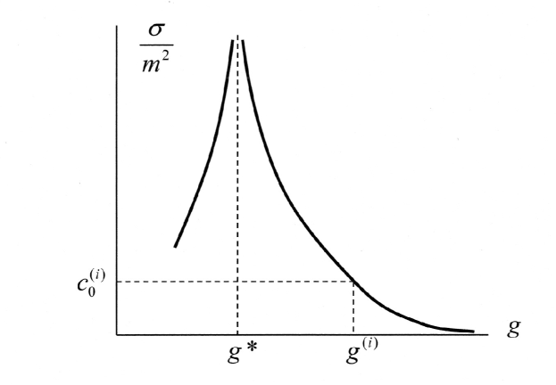
Figure 5: Dependence of $\sigma/m^{2}$ against $g$. In order to obtain the special values $c^{(i)}_{0}$, corresponding to zero values of the mass gap, one should mark all stable fixed points $g^{(i)}$ on the horizontal axis and make a construction shown in the figure.

Existence of points with $m=0$ in the parametric space means that the ”extended version” of Yang-Mills theory does not possess the mass gap. To eliminate this defect, we should return to the standard variant of theory, fixing one relation between observable quantities. The character of such relations is well-known and is determined by the so called ”dimensional transmutation” [16, Sec.14.1], [23, Sec.IV.6]. If we have $A=a^{\mu}f(g_{0})$ for the observable quantity $A$, then its independence of $a$ means

$$\frac{dA}{da}=\mu a^{\mu-1}f(g_{0})+a^{\mu}\,\frac{df(g_{0})}{dg_{0}^{2}}\,\frac{dg_{0}^{2}}{da}=a^{\mu-1}\left[\mu\,f(g_{0})-2\,\frac{df(g_{0})}{dg_{0}^{2}}\,\beta(g_{0}^{2})\right]=0\,,$$

where Eq.15 is taken into account. Integration of the obtained equation for $f(g_{0})$ gives

$$A=const\,a^{\mu}\exp\left\{\frac{\mu}{2}\,B(g_{0}^{2})\right\}\,,\qquad B(g_{0}^{2})=\int\,\frac{dg_{0}^{2}}{\beta(g_{0}^{2})}\,,$$

i.e. all quantities of the same dimensionality differ only by the constant factor, independent of $g_{0}$. For our purposes it is convenient to accept the condition

$$\sigma/m^{2}=c\,,$$

which defines the one-parameter family of Yang-Mills theories with different value of the structural constant $c$.  Under condition (24), the points with $m=0$, $\sigma=const$ become inaccessible.

It does not yet prove the existence of a mass gap, since $\sigma$ and $m$ can vanish simultaneously. In order to analyze such situations, consider the Gell-Mann – Low equation for the renormalized charge $g$ attributed to the scale $m$

$$\frac{d\,g^{2}}{d\,\ln m^{2}}=\beta(g^{2})=\beta_{0}g^{4}+\beta_{1}g^{6}+\ldots\,,$$

where $\beta$-function does not coincide with (15), but has the same first coefficients $\beta_{0}$ and $\beta_{1}$. It is clear that value $g^{*}$ (Fig.5) is a root of $\beta(g^{2})$; generally, it has several roots determining the RG fixed points. In the limit $m\to 0$, the charge $g$ tends to one of these fixed points, while following variants are possible for $\sigma/m^{2}$: (a) $\sigma/m^{2}\to\infty$, (b) $\sigma/m^{2}\to 0$, (c) $\sigma/m^{2}\to c_{0}$. The first two variants are incompatible with Eq.24, while the third variant is possible in the case $c=c_{0}$. If there are several stable fixed points $g^{(i)}$, then there are several special values $c^{(i)}_{0}$ (see Fig.5), for which the mass gap vanishes; for all other values of $c$ the mass gap is finite.

Physically, it looks most probable  that only one fixed point $g^{*}$ with $\sigma/m^{2}\to\infty$ is present, so no special values $c^{(i)}_{0}$ arise. Mathematically, one can suggest an infinite number of fixed points, which form a sequence $c^{(i)}_{0}$ everywhere dense in the interval $(0,\infty)$. However, small values of $\sigma/m^{2}$ correspond to the Wilson regime where finiteness of $\sigma$ and $m$ is verified immediately. As a result, the proof of the mass gap is complete for small values of the structural constant $c$.  The real perspective to strengthen this statement is outlined in Footnote 6.

It is worthwhile to indicate the papers [6, 24], which deal with $\beta$-functions, close to (25). The paper [24] considers $\beta(g^{2})$ defined in the $MS$-scheme, where differentiation in (25) is performed over arbitrary momentum scale $\mu$; behavior $\beta(g^{2})=\beta_{\infty}g^{2\alpha}$ with $\alpha\approx-13$ is obtained for large $g$, while the sign of $\beta_{\infty}$ remained indefinite, so existence of fixed point is one of the possible variants. Alternative definition of $\beta(g^{2})$ can be obtained in QCD, if $g$ is attributed to the scale of the quark mass $m$; if $g$ is defined through the quark-gluon vertex, then calculation of the asymptotics for $\beta$-function can be performed in a complete analogue with QED [6], giving result $\beta(g^{2})=g^{2}$ with necessary existence of a fixed point. We have seen above the existence of fixed point when the glueball mass $m$ was making the scale. The listed definitions of $\beta(g^{2})$ are different technically, but physically correspond to the same dependence of renormalized charge on the length scale . The physical sense of existence of fixed point was clarified above.

If massless quarks  are introduced, then the regime of dimensional transmutation is conserved and the trick with ”extension” of theory remains actual; it seems, that the general structure of theory is also retained.

Our final conclusions are as follows:

Whatever are properties of continuous Yang-Mills theory, there exists a lattice theory, which reproduces them. The bare charge $g_{0}$ in this lattice theory can be taken arbitrary, and in particular infinitely large. Any reasonable lattice version of Yang-Mills theory gives finite values of $\sigma$ and $m$ in the strong coupling limit. Vanishing of $\sigma$ and $m$ is possible for exceptional configurations in many-parameter space, which are avoided in the general situation. As a result, the problem of analytical proof of confinement and the mass gap can be considered as solved, at least on the physical level of rigor.

References

- [1] I. M. Suslov, Zh. Eksp. Teor. Fiz. 120, 5 (2001) [JETP 93, 1 (2001)].
- [2] I. M. Suslov, Zh. Eksp. Teor. Fiz. 134, 490 (2008) [JETP 107, 413 (2008)].
- [3] I. M. Suslov, Zh. Eksp. Teor. Fiz. 138, 508 (2010) [JETP 111, 450 (2010)].
- [4] I. M. Suslov, Zh. Eksp. Teor. Fiz. 139, 319 (2011). [JETP 112, 274 (2011)].
- [5] I. M. Suslov, Zh. Eksp. Teor. Fiz. 127, 1350 (2005) [JETP 100, 1188 (2005)].
- [6] I. M. Suslov, Zh. Eksp. Teor. Fiz. 135, 1129 (2009) [JETP 108, 980 (2009)].
- [7] N. N. Bogolyubov and D. V. Shirkov, Introduction to the Theory of Quantized Fields, 3rd ed. (Nauka, Moscow, 1976; Wiley, New York, 1980).
- [8] K. G. Wilson and J. Kogut, Phys. Rep. C 12, 75 (1975).
- [9] J. Frlich, Nucl. Phys. B 200 [FS4], 281 (1982).
- [10] M. Aizenman, Commun. Math. Soc. 86, 1 (1982).
- [11] B. Freedman, P. Smolensky, D. Weingarten, Phys. Lett. B 113, 481 (1982).
- [12] M. Lscher, P. Weisz, Nucl. Phys. B 290 [FS20], 25 (1987); 295 [FS21], 65 (1988); 318, 705 (1989).
- [13] I. M. Suslov, arXiv: 0806.0789.
- [14] R. F. Dashen, H. Neuberger, Phys. Rev. Lett. 50, 1897 (1983).
- [15] E. Abrahams, P. W. Anderson, D. C. Licciardello, and T. V. Ramakrishman, Phys. Rev. Lett. 42, 673 (1979).
- [16] R. Gupta, arXiv: hep-lat/9807028.
- [17] S. Coleman, E. Weinberg, Phys. Rev. D 7, 1888 (1973).
- [18] K. G. Wilson , Phys. Rev. D 10, 2445 (1974).
- [19] M. Creutz, Quarks, gluons and lattices, Cambridge University Press, 1983.
- [20] A. A. Vladimirov and D. V. Shirkov, Usp. Fiz. Nauk 129, 407 (1979) [Sov. Phys. Usp. 22, 860 (1979)].
- [21] C. Callan, R. Dashen, D. Gross, Phys. Rev. D 20, 3279 (1979).
- [22] J. B. Kogut, R. B. Pearson, J. Shigemitsu, Phys. Rev. Lett. 43, 484 (1979).
- [23] A. A. Slavnov, L. D. Faddeev. Introduction to Quantum Theory of Gauge Fields (Nauka, Moscow, 1988).
- [24] I. M. Suslov, Pis’ma Zh. Eksp. Teor. Fiz. 76, 387 (2002) [JETP Lett. 76, 327 (2002)].
- [25] I. M. Suslov, arXiv: hep-ph/0605115.