Data Separation by Sparse Representations

Abstract

Recently, sparsity has become a key concept in various areas of applied mathematics, computer science, and electrical engineering. One application of this novel methodology is the separation of data, which is composed of two (or more) morphologically distinct constituents. The key idea is to carefully select representation systems each providing sparse approximations of one of the components. Then the sparsest coefficient vector representing the data within the composed – and therefore highly redundant – representation system is computed by $\ell_{1}$ minimization or thresholding. This automatically enforces separation.

This paper shall serve as an introduction to and a survey about this exciting area of research as well as a reference for the state-of-the-art of this research field.

Key Words. Coherence. $\ell_{1}$ minimization. Morphology. Separation. Sparse Representation. Tight Frames.

Acknowledgements. The author would like to thank Ronald Coifman, Michael Elad, and Remi Gribonval for various discussions on related topics, and Wang-Q Lim for producing Figures 2, 3, and 5. Special thanks go to David Donoho for a great collaboration on topics in this area and enlightening debates, and to Michael Elad for very useful comments on an earlier version of this survey. The author is also grateful to the Department of Statistics at Stanford University and the Mathematics Department at Yale University for their hospitality and support during her visits. She acknowledges support by Deutsche Forschungsgemeinschaft (DFG) Heisenberg fellowship KU 1446/8, DFG Grant SPP-1324 KU 1446/13, and DFG Grant KU 1446/14.

1 Introduction

Over the last years, scientists face an ever growing deluge of data, which needs to be transmitted, analyzed, and stored. A close analysis reveals that most of these data might be classified as multimodal data, i.e., being composed of distinct subcomponents. Prominent examples are audio data, which might consist of a superposition of the sounds of different instruments, or imaging data from neurobiology, which is typically a composition of the soma of a neuron, its dendrites, and its spines. In both these exemplary situations, the data has to be separated into appropriate single components for further analysis. In the first case, separating the audio signal into the signals of the different instruments is a first step to enable the audio technician to obtain a musical score from a recording. In the second case, the neurobiologist might aim to analyze the structure of dendrites and spines separately for the study of Alzheimer specific characteristics. Thus data separation is often a crucial step in the analysis of data.

As a scientist, three fundamental problems immediately come to one’s mind:

1. What is a mathematically precise meaning of the vague term ‘distinct components’?

2. How do we separate data algorithmically?

3. When is separation possible at all?

To answer those questions, we need to first understand the key problem in data separation. In a very simplistic view, the essence of the problem is as follows: Given a composed signal $x$ of the form $x=x_{1}+x_{2}$, we aim to extract the unknown components $x_{1}$ and $x_{2}$ from it. Having one known data and two unknowns obviously makes this problem underdetermined. Thus, the novel paradigm of sparsity – appropriately utilized – seems a perfect fit for attacking data separation, and this chapter shall serve as both an introduction into this intriguing application of sparse representations as well as a reference for the state-of-the-art of this research area.

1.1 Morphological Component Analysis

Intriguingly, when considering the history of Compressed Sensing, the first mathematically precise result on recovery of sparse vectors by $\ell_{1}$ minimization is related to a data separation problem: The separation of sinusoids and spikes in [16, 11]. Thus it might be considered a milestone in the development of Compressed Sensing. In addition, it reveals a surprising connection with uncertainty principles.

The general idea allowing separation in [16, 11] was to choose two bases or frames $\Phi_{1}$ and $\Phi_{2}$ adapted to the two components to be separated in such a way that $\Phi_{1}$ and $\Phi_{2}$ provide a sparse representation for $x_{1}$ and $x_{2}$, respectively. Searching for the sparsest representation of the signal in the combined (highly overcomplete) dictionary $[\>\Phi_{1}\>|\>\Phi_{2}\>]$ should then intuitively enforce separation provided that $x_{1}$ does not have a sparse representation in $\Phi_{2}$ and that $x_{2}$ does not have a sparse representation in $\Phi_{1}$. This general concept was later – in the context of image separation, but the term seems to be fitting in general – coined Morphological Component Analysis [36].

This viewpoint now measures the morphological difference between components in terms of the incoherence of suitable sparsifying bases or frames $\Phi_{i}$, thereby giving one possible answer to (P1); see also the respective chapters in the novel book [33]. One possibility for measuring incoherence is the mutual coherence. We will however see in the sequel that there exist even more appropriate coherence notions, which provide a much more refined measurement of incoherence specifically adapted to measuring morphological difference.

1.2 Separation Algorithms

Going again back in time, we observe that far before [11], Coifman, Wickerhauser, and co-workers already presented very inspiring empirical results on the separation of image components using the idea of Morphological Component Analysis, see [7]. After this, several techniques to actually compute the sparsest expansion in a composed dictionary $[\>\Phi_{1}\>|\>\Phi_{2}\>]$ were introduced. In [31], Mallat and Zhang developed Matching Pursuit as one possible methodology. The study by Chen, Donoho, and Saunders in [6] then revealed that the $\ell_{1}$ norm has a tendency to find sparse solutions when they exist, and coined this method Basis Pursuit.

As explained before, data separation by Morphological Component Analysis – when suitably applied – can be reduced to a sparse recovery problem. To solve this problem, there nowadays already exist a variety of utilizable algorithmic approaches; thereby providing a general answer to (P2). Such approaches include, for instance, a canon of greedy-type algorithms. Most of the theoretical separation results however consider $\ell_{1}$ minimization as the main separation technique, which is what we will also mainly focus on in this chapter.

1.3 Separation Results

As already mentioned, the first mathematically precise result was derived in [11] and solved the problem of separation of sinusoids and spikes. After this ‘birth of sparse data separation’, a deluge of very exciting results started. One direction of research are general results on sparse recovery and Compressed Sensing; here we would like to cite the excellent survey paper [4].

Another direction continued the idea of sparse data separation initiated in [11]. In this realm, the most significant theoretical results might be considered firstly the series of papers [19, 10], in which the initial results from [11] are extended to general composed dictionaries, secondly the paper [23], which also extends results from [11] though with a different perspective, and thirdly the papers [3] and [14], which explore the clustering of the sparse coefficients and the morphological difference of the components encoded in it.

We also wish to mention the abundance of empirical work showing that utilizing the idea of sparse data separation often gives very compelling results in practice, as examples, we refer to the series of papers on applications to astronomical data [2, 36, 34], to general imaging data [32, 20, 35], and to audio data [22, 25].

Let us remark that also the classical problem of denoising can be regarded as a separation problem, since we aim to separate a signal from noise by utilizing the characteristics of the signal family and the noise. However, as opposed to the separation problems discussed in this chapter, denoising is not a ‘symmetric’ separation task, since the characterization of the signal and the noise are very different.

1.4 Design of Sparse Dictionaries

For satisfactorily answering (P3), one must also raise the question of how to find suitable sparsifying bases or frames for given components. This search for ‘good’ systems in the sense of sparse dictionaries can be attacked in two ways, either non-adaptively or adaptively.

The first path explores the structure of the component one would like to extract, for instance, it could be periodic such as sinusoids or anisotropic such as edges in images. This typically allows one to find a suitable system among the already very well explored representation systems such as the Fourier basis, wavelets, or shearlets, to name a few. The advantage of this approach is the already explored structure of the system, which can hence be exploited for deriving theoretical results on the accuracy of separation, and the speed of associated transforms.

The second path uses a training set of data similar to the to-be-extracted component, and ‘learns’ a system which best sparsifies this data set. Using this approach customarily referred to as dictionary learning, we obtain a system extremely well adapted to the data at hand; as the state-of-the-art we would like to mention the K-SVD algorithm introduced by Aahron, Elad, and Bruckstein in [1]; see also [17] for a ‘Compressed Sensing’ perspective to K-SVD. Another appealing dictionary training algorithm, which should be cited is the method of optimal directions (MOD) by Engan et al. [21]. The downside however is the lack of a mathematically exploitable structure, which makes a theoretical analysis of the accuracy of separation using such a system very hard.

1.5 Outline

In Section 2, we discuss the formal mathematical setting of the problem, present the nowadays already considered classical separation results, and then discuss more recent results exploiting the clustering of significant coefficients in the expansions of the components as a means to measure their morphological difference. We conclude this section by revealing a close link of data separation to uncertainty principles. Section 3 is then devoted to both theoretical results as well as applications for separation of 1D signals, elaborating, in particular, on the separation of sinusoids and spikes. Finally, Section 4 focuses on diverse questions concerning separation of 2D signals, i.e., images, such as the separation of point- and curvelike objects, again presenting both application aspects as well as theoretical results.

2 Separation Estimates

As already mentioned in the introduction, data separation can be regarded within the framework of underdetermined problems. In this section, we make this link mathematically precise. Then we discuss general estimates on the separability of composed data, firstly without any knowledge of the geometric structure of sparsity patterns, and secondly, by taking known geometric information into account. A revelation of the close relation with uncertainty principles concludes the section.

In Sections 3 and 4, we will then see the presented general results and uncertainty principles in action, i.e., applied to real-world separation problems.

2.1 Relation with Underdetermined Problems

Let $x$ be our signal of interest, which we for now consider as belonging to some Hilbert space $\mathcal{H}$, and assume that

$$x=x_{1}^{0}+x_{2}^{0}.$$

Certainly, real data is typically composed of multiple components, hence not only the situation of two components, but three or more is of interest. We will however focus on the two-component situation to clarify the fundamental principles behind the success of separating those by sparsity methodologies. It should be mentioned though that, in fact, most of the presented theoretical results can be extended to the multiple component situation in a more or less straightforward manner.

To extract the two components from $x$, we need to assume that – although we are not given $x_{1}^{0}$ and $x_{2}^{0}$ – certain ‘characteristics’ of those components are known to us. Such ‘characteristics’ might be, for instance, the pointlike structure of stars and the curvelike structure of filaments in astronomical imaging. This knowledge now enables us to choose two representation systems, $\Phi_{1}$ and $\Phi_{2}$, say, which allow sparse expansions of $x_{1}^{0}$ and $x_{2}^{0}$, respectively. Such representation systems might be chosen from the collection of well-known systems such as wavelets. A different possibility is to choose adaptively the systems via dictionary learning procedures. This approach however requires training data sets for the two components $x_{1}^{0}$ and $x_{2}^{0}$ as discussed in Subsection 1.4.

Given now two such representation systems $\Phi_{1}$ and $\Phi_{2}$, we can write $x$ as

$$x=x_{1}^{0}+x_{2}^{0}=\Phi_{1}c_{1}^{0}+\Phi_{2}c_{2}^{0}=[\>\Phi_{1}\>|\>\Phi_{2}\>]\left[\begin{array}[]{c}c_{1}^{0}\\ c_{2}^{0}\end{array}\right]$$

with $\|c_{1}^{0}\|_{0}$ and $\|c_{2}^{0}\|_{0}$ ‘sufficiently small’. Thus, the data separation problem has been reduced to solving the underdetermined linear system

$$x=[\>\Phi_{1}\>|\>\Phi_{2}\>]\left[\begin{array}[]{c}c_{1}\\ c_{2}\end{array}\right]$$ (1)

for $[c_{1},c_{2}]^{T}$. Unique recovery of the original vector $[c_{1}^{0},c_{2}^{0}]^{T}$ automatically extracts the correct two components $x_{1}^{0}$ and $x_{2}^{0}$ from $x$, since

$$x_{1}^{0}=\Phi_{1}c_{1}^{0}\quad\mbox{and}\quad x_{2}^{0}=\Phi_{2}c_{2}^{0}.$$

Ideally, one might want to solve

$$\min_{c_{1},c_{2}}\|c_{1}\|_{0}+\|c_{2}\|_{0}\quad\textrm{s.t.}\quad x=[\>\Phi_{1}\>|\>\Phi_{2}\>]\left[\begin{array}[]{c}c_{1}\\ c_{2}\end{array}\right],$$ (2)

which however is an NP-hard problem. Instead one aims to solve the $\ell_{1}$ minimization problem

$$(\mbox{Sep}_{s})\qquad\min_{c_{1},c_{2}}\|c_{1}\|_{1}+\|c_{2}\|_{1}\quad\textrm{s.t.}\quad x=[\>\Phi_{1}\>|\>\Phi_{2}\>]\left[\begin{array}[]{c}c_{1}\\ c_{2}\end{array}\right].$$ (3)

The lower case ‘s’ in $\mbox{Sep}_{s}$ indicates that the $\ell_{1}$ norm is placed on the synthesis side. Other choices for separation are, for instance, greedy-type algorithms. In this chapter we will focus on $\ell_{1}$ minimization as the separation technique, consistent with most known separation results from the literature.

Before discussing conditions on $[c_{1}^{0},c_{2}^{0}]^{T}$ and $[\>\Phi_{1}\>|\>\Phi_{2}\>]$, which guarantee unique solvability of (1), let us for a moment debate whether uniqueness is necessary at all. If $\Phi_{1}$ and $\Phi_{2}$ form bases, it is certainly essential to recover $[c_{1}^{0},c_{2}^{0}]^{T}$ uniquely from (1). However, some well-known representation systems are in fact redundant and typically constitute Parseval frames such as curvelets or shearlets. Also, systems generated by dictionary learning are normally highly redundant. In this situation, for each possible separation

$$x=x_{1}+x_{2},$$ (4)

there exist infinitely many coefficient sequences $[c_{1},c_{2}]^{T}$ satisfying

$$x_{1}=\Phi_{1}c_{1}\quad\mbox{and}\quad x_{2}=\Phi_{2}c_{2}.$$ (5)

Since we are only interested in the correct separation and not in computing the sparsest expansion, we can circumvent presumably arising numerical instabilities when solving the minimization problem (3) by selecting a particular coefficient sequence for each separation. Assuming $\Phi_{1}$ and $\Phi_{2}$ are Parseval frames, we can exploit this structure and rewrite (5) as

$$x_{1}=\Phi_{1}(\Phi_{1}^{T}x_{1})\quad\mbox{and}\quad x_{2}=\Phi_{2}(\Phi_{2}^{T}x_{2}).$$

Thus, for each separation (4), we choose a specific coefficient sequence when expanding the components in the Parseval frames, in fact, we choose the analysis sequence. This leads to the following different $\ell_{1}$ minimization problem in which the $\ell_{1}$ norm is placed on the analysis rather than the synthesis side:

$$(\mbox{Sep}_{a})\qquad\min_{x_{1},x_{2}}\|\Phi_{1}^{T}x_{1}\|_{1}+\|\Phi_{2}^{T}x_{2}\|_{1}\quad\textrm{s.t.}\quad x=x_{1}+x_{2}.$$ (6)

This new minimization problem can be also regarded as a mixed $\ell_{1}$-$\ell_{2}$ problem, since the analysis coefficient sequence is exactly the coefficient sequence which is minimal in the $\ell_{2}$ norm.

2.2 General Separation Estimates

Let us now discuss the main results of successful data separation, i.e., stating conditions on $[c_{1}^{0},c_{2}^{0}]^{T}$ and $[\>\Phi_{1}\>|\>\Phi_{2}\>]$ for extracting $x_{1}^{0}$ and $x_{2}^{0}$ from $x$. The strongest known general result was derived in 2003 by Donoho and Elad [10] and used the notion of mutual coherence. Recall that, for a normalized frame $\Phi=(\varphi_{i})_{i\in I}$, the mutual coherence of $\Phi$ is defined by

$$\mu(\Phi)=\max_{i,j\in I,i\neq j}|\langle\varphi_{i},\varphi_{j}\rangle|.$$

The result states the following.

Theorem 2.1 ([10])

Let $\Phi_{1}$ and $\Phi_{2}$ be two frames for a Hilbert space $\mathcal{H}$, and let $x\in\mathcal{H}$, $x\neq 0$. If $x=[\Phi_{1}|\Phi_{2}]c$ and

$$\|c\|_{0}<\frac{1}{2}\left(1+\frac{1}{\mu([\Phi_{1}|\Phi_{2}])}\right),$$

then the solution of the $\ell_{1}$ minimization problem $(\mbox{Sep}_{s})$ stated in (3) coincides with the solution of the $\ell_{0}$ minimization problem stated in (2).

Before presenting the proof, we require some prerequisites. Firstly, we need to introduce the so-called nullspace property.

Definition 2.2

Let $\Phi=(\varphi_{i})_{i\in I}$ be a frame for a Hilbert space $\mathcal{H}$, and let ${\mathcal{N}}(\Phi)$ denote the null space of $\Phi$. Then $\Phi$ is said to have the null space property of order $k$ if

$$\|1_{\Lambda}d\|_{1}<\frac{1}{2}\|d\|_{1}$$

for all $d\in{\mathcal{N}}(\Phi)\setminus\{0\}$ and for all sets $\Lambda\subseteq I$ with $|\Lambda|\leq k$.

This notion provides a very useful characterization of the existence of unique sparse solutions of the $\ell_{1}$ minimization problem $(\mbox{Sep}_{s})$ stated in (3).

Lemma 2.3

Let $\Phi=(\varphi_{i})_{i\in I}$ be a frame for a Hilbert space $\mathcal{H}$, and let $x\in\mathcal{H}$. Then the following conditions are equivalent.

1. All vectors $c$ with $\|c\|_{0}\leq k$ are unique solutions of the $\ell_{1}$ minimization problem $(\mbox{Sep}_{s})$ stated in (3) (with $\Phi$ instead of $[\Phi_{1}|\Phi_{2}]$).

2. $\Phi$ satisfies the null space property of order $k$.

Proof. First, assume that (i) holds. Let $d\in{\mathcal{N}}(\Phi)\setminus\{0\}$ and $\Lambda\subseteq I$ with $|\Lambda|\leq k$ be arbitrary. Then, by (i), the sparse vector $1_{\Lambda}d$ is the unique minimizer of $\|c\|_{1}$ subject to $\Phi c=\Phi(1_{\Lambda}d)$. Further, since $d\in{\mathcal{N}}(\Phi)\setminus\{0\}$,

$$\Phi(-1_{\Lambda^{c}}d)=\Phi(1_{\Lambda}d).$$

Hence

$$\|1_{\Lambda}d\|_{1}<\|1_{\Lambda^{c}}d\|_{1},$$

or, in other words,

$$\|1_{\Lambda}d\|_{1}<\frac{1}{2}\|d\|_{1},$$

which implies (ii), since $d$ and $\Lambda$ were chosen arbitrarily.

Secondly, assume that (ii) holds, and let $c_{1}$ be a vector with $\|c_{1}\|_{0}\leq k$ and support denoted by $\Lambda$. Further, let $c_{2}$ be an arbitrary solution of $x=\Phi c$, and set

$$d=c_{2}-c_{1}.$$

Then

$$\|c_{2}\|_{1}-\|c_{1}\|_{1}=\|1_{\Lambda^{c}}c_{2}\|_{1}+\|1_{\Lambda}c_{2}\|_{1}-\|1_{\Lambda}c_{1}\|_{1}\geq\|1_{\Lambda^{c}}d\|_{1}-\|1_{\Lambda}d\|_{1}.$$

This term is greater than zero for any $d\neq 0$ if

$$\|1_{\Lambda^{c}}d\|_{1}>\|1_{\Lambda}d\|_{1},$$

or

$$\frac{1}{2}\|d\|_{1}>\|1_{\Lambda}d\|_{1}.$$

This is ensured by (ii). Hence $\|c_{2}\|_{1}>\|c_{1}\|_{1}$, and thus $c_{1}$ is the unique solution of $(\mbox{Sep}_{s})$. This implies (i). $\Box$

Using this result, we next prove that a solution satisfying $\|c\|_{0}<\frac{1}{2}\left(1+\frac{1}{\mu(\Phi)}\right)$ is the unique solution of the $\ell_{1}$ minimization problem $(\mbox{Sep}_{s})$.

Lemma 2.4

Let $\Phi=(\varphi_{i})_{i\in I}$ be a frame for a Hilbert space $\mathcal{H}$, and let $x\in\mathcal{H}$. If $c$ is a solution of the $\ell_{1}$ minimization problem $(\mbox{Sep}_{s})$ stated in (3) (with $\Phi$ instead of $[\Phi_{1}|\Phi_{2}]$) and satisfies

$$\|c\|_{0}<\frac{1}{2}\left(1+\frac{1}{\mu(\Phi)}\right),$$

then it is the unique solution.

Proof. Let $d\in{\mathcal{N}}(\Phi)\setminus\{0\}$, hence, in particular,

$$\Phi d=0;$$

thus also

$$\Phi^{\star}\Phi d=0.$$ (7)

Without loss of generality, we now assume that the vectors in $\Phi$ are normalized. Then, (7) implies that, for all $i\in I$,

$$d_{i}=-\sum_{j\neq i}\langle\varphi_{i},\varphi_{j}\rangle d_{j}.$$

Using the definition of mutual coherence $\mu(\Phi)$ (cf. Subsection 2.2), we obtain

$$|d_{i}|\leq\sum_{j\neq i}|\langle\varphi_{i},\varphi_{j}\rangle|\cdot|d_{j}|\leq\mu(\Phi)(\|d\|_{1}-|d_{i}|),$$

and hence

$$|d_{i}|\leq\left(1+\frac{1}{\mu(\Phi)}\right)^{-1}\|d\|_{1}.$$

Thus, by the hypothesis on $\|c\|_{0}$ and for any $\Lambda\subseteq I$ with $|\Lambda|=\|c\|_{0}$, we have

$$\|1_{\Lambda}d\|_{1}\leq|\Lambda|\cdot\left(1+\frac{1}{\mu(\Phi)}\right)^{-1}\|d\|_{1}=\|c\|_{0}\cdot\left(1+\frac{1}{\mu(\Phi)}\right)^{-1}\|d\|_{1}<\frac{1}{2}\|d\|_{1}.$$

This shows that $\Phi$ satisfies the null space property of order $\|c\|_{0}$, which, by Lemma 2.3, implies that $c$ is the unique solution of $(\mbox{Sep}_{s})$. $\Box$

We further prove that a solution satisfying $\|c\|_{0}<\frac{1}{2}\left(1+\frac{1}{\mu(\Phi)}\right)$ is also the unique solution of the $\ell_{0}$-minimization problem.

Lemma 2.5

Let $\Phi=(\varphi_{i})_{i\in I}$ be a frame for a Hilbert space $\mathcal{H}$, and let $x\in\mathcal{H}$. If $c$ is a solution of the $\ell_{0}$ minimization problem stated in (2) (with $\Phi$ instead of $[\Phi_{1}|\Phi_{2}]$) and satisfies

$$\|c\|_{0}<\frac{1}{2}\left(1+\frac{1}{\mu(\Phi)}\right),$$

then it is the unique solution.

Proof. By Lemma 2.4, the hypotheses imply that $c$ is the unique solution of the $\ell_{1}$ minimization problem $(\mbox{Sep}_{s})$. Now, towards a contradiction, assume that there exists some $\tilde{c}$ satisfying $x=\Phi\tilde{c}$ with $\|\tilde{c}\|_{0}\leq\|c\|_{0}$. Then $\tilde{c}$ must satisfy

$$\|\tilde{c}\|_{0}<\frac{1}{2}\left(1+\frac{1}{\mu(\Phi)}\right).$$

Again, by Lemma 2.4, $\tilde{c}$ is the unique solution of the $\ell_{1}$ minimization problem $(\mbox{Sep}_{s})$, a contradiction. $\Box$

These lemmata now immediately imply Theorem 2.1.

Proof [Proof of Theorem 2.1]. Theorem 2.1 follows from Lemmata 2.4 and 2.5. $\Box$

Interestingly, in the situation of $\Phi_{1}$ and $\Phi_{2}$ being two orthonormal bases the bound can be slightly strengthened. For the proof of this result, we refer the reader to [19].

Theorem 2.6 ([19])

Let $\Phi_{1}$ and $\Phi_{2}$ be two orthonormal bases for a Hilbert space $\mathcal{H}$, and let $x\in\mathcal{H}$. If $x=[\Phi_{1}|\Phi_{2}]c$ and

$$\|c\|_{0}<\frac{\sqrt{2}-0.5}{\mu([\Phi_{1}|\Phi_{2}])},$$

then the solution of the $\ell_{1}$ minimization problem $(\mbox{Sep}_{s})$ stated in (3) coincides with the solution of the $\ell_{0}$ minimization problem stated in (2).

This shows that in the special situation of two orthonormal bases, the bound is nearly a factor of $2$ stronger than in the general situation of Theorem 2.1.

2.3 Clustered Sparsity as a Novel Viewpoint

In a concrete situation, we often have more information on the geometry of the to-be-separated components $x_{1}^{0}$ and $x_{2}^{0}$. This information is typically encoded in a particular clustering of the non-zero coefficients if a suitable basis or frame for the expansion of $x_{1}^{0}$ or $x_{2}^{0}$ is chosen. Think, for instance, of the tree clustering of wavelet coefficients of a point singularity. Thus, it seems conceivable that the morphological difference is encoded not only in the incoherence of the two chosen bases or frames adapted to $x_{1}^{0}$ and $x_{2}^{0}$, but in the interaction of the elements of those bases or frames associated with the clusters of significant coefficients. This should intuitively allow for weaker necessary conditions for separation.

One possibility for a notion capturing this idea is the so-called joint concentration which was introduced in [14] with concepts going back to [16], and was in between again revived in [11]. To provide some intuition for this notion, let $\Lambda_{1}$ and $\Lambda_{2}$ be subsets of indexing sets of two Parseval frames. Then the joint concentration measures the maximal fraction of the total $\ell_{1}$ norm which can be concentrated on the index set $\Lambda_{1}\cup\Lambda_{2}$ of the combined dictionary.

Definition 2.7

Let $\Phi_{1}=(\varphi_{1i})_{i\in I}$ and $\Phi_{2}=(\varphi_{2j})_{j\in J}$ be two Parseval frames for a Hilbert space $\mathcal{H}$. Further, let $\Lambda_{1}\subseteq I$ and $\Lambda_{2}\subseteq J$. Then the joint concentration $\kappa=\kappa(\Lambda_{1},\Phi_{1};\Lambda_{2},\Phi_{2})$ is defined by

$$\kappa(\Lambda_{1},\Phi_{1};\Lambda_{2},\Phi_{2})=\sup_{x}\frac{\|1_{\Lambda_{1}}\Phi_{1}^{T}x\|_{1}+\|1_{\Lambda_{2}}\Phi_{2}^{T}x\|_{1}}{\|\Phi_{1}^{T}x\|_{1}+\|\Phi_{2}^{T}x\|_{1}}.$$

One might ask how the notion of joint concentration relates to the widely exploited, and for the previous result utilized mutual coherence. For this, we first briefly discuss some derivations of mutual coherence. A first variant better adapted to clustering of coefficients was the Babel function first introduced in [10] and later in [37] under the label cumulative coherence function, which, for a normalized frame $\Phi=(\varphi_{i})_{i\in I}$ and some $m\in\{1,\ldots,|I|\}$ is defined by

$$\mu_{B}(m,\Phi)=\max_{\Lambda\subset I,|\Lambda|=m}\max_{j\not\in\Lambda}\sum_{i\in I}|\langle\varphi_{i},\varphi_{j}\rangle|.$$

This notion was later refined in [3] by considering the so-called structured $p$-Babel function, defined for some family ${\mathcal{S}}$ of subsets of $I$ and some $1\leq p<\infty$ by

$$\mu_{sB}({\mathcal{S}},\Phi)=\max_{\Lambda\in{\mathcal{S}}}\left(\max_{j\not\in\Lambda}\sum_{i\in I}|\langle\varphi_{i},\varphi_{j}\rangle|^{p}\right)^{1/p}.$$

Another variant, better adapted to data separation, is the cluster coherence introduced in [14], whose definition we now formally state. Notice that we do not assume that the vectors are normalized.

Definition 2.8

Let $\Phi_{1}=(\varphi_{1i})_{i\in I}$ and $\Phi_{2}=(\varphi_{2j})_{j\in J}$ be two Parseval frames for a Hilbert space $\mathcal{H}$, let $\Lambda_{1}\subseteq I$, and let $\Lambda_{2}\subseteq J$. Then the cluster coherence $\mu_{c}(\Lambda_{1},\Phi_{1};\Phi_{2})$ of $\Phi_{1}$ and $\Phi_{2}$ with respect to $\Lambda_{1}$ is defined by

$$\mu_{c}(\Lambda_{1},\Phi_{1};\Phi_{2})=\max_{j\in J}\sum_{i\in\Lambda_{1}}|\langle\varphi_{1i},\varphi_{2j}\rangle|,$$

and the cluster coherence $\mu_{c}(\Phi_{1};\Lambda_{2},\Phi_{2})$ of $\Phi_{1}$ and $\Phi_{2}$ with respect to $\Lambda_{2}$ is defined by

$$\mu_{c}(\Phi_{1};\Lambda_{2},\Phi_{2})=\max_{i\in I}\sum_{j\in\Lambda_{2}}|\langle\varphi_{1i},\varphi_{2j}\rangle|.$$

The relation between joint concentration and cluster coherence is made precise in the following result from [14].

Proposition 2.9 ([14])

Let $\Phi_{1}=(\varphi_{1i})_{i\in I}$ and $\Phi_{2}=(\varphi_{2j})_{j\in J}$ be two Parseval frames for a Hilbert space $\mathcal{H}$, and let $\Lambda_{1}\subseteq I$ and $\Lambda_{2}\subseteq J$. Then

$$\kappa(\Lambda_{1},\Phi_{1};\Lambda_{2},\Phi_{2})\leq\max\{\mu_{c}(\Lambda_{1},\Phi_{1};\Phi_{2}),\mu_{c}(\Phi_{1};\Lambda_{2},\Phi_{2})\}.$$

Proof. Let $x\in\mathcal{H}$. We now choose coefficient sequences $c_{1}$ and $c_{2}$ such that

$$x=\Phi_{1}c_{1}=\Phi_{2}c_{2}$$

and, for $i=1,2$,

$$\|c_{i}\|_{1}\leq\|d_{i}\|_{1}\quad\mbox{for all }d_{i}\mbox{ with }x=\Phi_{i}d_{i}.$$ (8)

This implies that

$$\|1_{\Lambda_{1}}\Phi_{1}^{T}x\|_{1}+\|1_{\Lambda_{2}}\Phi_{2}^{T}x\|_{1}$$

$$= \|1_{\Lambda_{1}}\Phi_{1}^{T}\Phi_{2}c_{2}\|_{1}+\|1_{\Lambda_{2}}\Phi_{2}^{T}\Phi_{1}c_{1}\|_{1}$$

$$\leq \sum_{i\in\Lambda_{1}}\left(\sum_{j\in J}|\langle\varphi_{1i},\varphi_{2j}\rangle||c_{2j}|\right)+\sum_{j\in\Lambda_{2}}\left(\sum_{i\in I}|\langle\varphi_{1i},\varphi_{2j}\rangle||c_{1i}|\right)$$

$$= \sum_{j\in J}\left(\sum_{i\in\Lambda_{1}}|\langle\varphi_{1i},\varphi_{2j}\rangle|\right)|c_{2j}|+\sum_{i\in I}\left(\sum_{j\in\Lambda_{2}}|\langle\varphi_{1i},\varphi_{2j}\rangle|\right)|c_{1i}|$$

$$\leq \mu_{c}(\Lambda_{1},\Phi_{1};\Phi_{2})\|c_{2}\|_{1}+\mu_{c}(\Lambda_{2},\Phi_{2};\Phi_{1})\|c_{1}\|_{1}$$

$$\leq \max\{\mu_{c}(\Lambda_{1},\Phi_{1};\Phi_{2}),\mu_{c}(\Lambda_{2},\Phi_{2};\Phi_{1})\}(\|c_{1}\|_{1}+\|c_{2}\|_{1}).$$

Since $\Phi_{1}$ and $\Phi_{2}$ are Parseval frames, we have

$$x=\Phi_{i}(\Phi_{i}^{T}\Phi_{i}c_{i})\quad\mbox{for }i=1,2.$$

Hence, by exploiting (8),

$$\|1_{\Lambda_{1}}\Phi_{1}^{T}x\|_{1}+\|1_{\Lambda_{2}}\Phi_{2}^{T}x\|_{1}$$

$$\leq \max\{\mu_{c}(\Lambda_{1},\Phi_{1};\Phi_{2}),\mu_{c}(\Lambda_{2},\Phi_{2};\Phi_{1})\}(\|\Phi_{1}^{T}\Phi_{1}c_{1}\|_{1}+\|\Phi_{2}^{T}\Phi_{2}c_{2}\|_{1})$$

$$= \max\{\mu_{c}(\Lambda_{1},\Phi_{1};\Phi_{2}),\mu_{c}(\Lambda_{2},\Phi_{2};\Phi_{1})\}(\|\Phi_{1}^{T}x\|_{1}+\|\Phi_{2}^{T}x\|_{1}).\quad\mbox{ $\Box$}$$

Before stating the data separation estimate which uses joint concentration, we need to discuss the conditions on sparsity of the components in the two Parseval frames. Since for real data ‘true sparsity’ is unrealistic, a weaker condition will be imposed. For the next result, a notion invoking the clustering of the significant coefficients will be required. This notion, first utilized in [9], is defined for our data separation problem as follows.

Definition 2.10

Let $\Phi_{1}=(\varphi_{1i})_{i\in I}$ and $\Phi_{2}=(\varphi_{2j})_{j\in J}$ be two Parseval frames for a Hilbert space $\mathcal{H}$, and let $\Lambda_{1}\subseteq I$ and $\Lambda_{2}\subseteq J$. Further, suppose that $x\in\mathcal{H}$ can be decomposed as $x=x_{1}^{0}+x_{2}^{0}$. Then the components $x_{1}^{0}$ and $x_{2}^{0}$ are called $\delta$-relatively sparse in $\Phi_{1}$ and $\Phi_{2}$ with respect to $\Lambda_{1}$ and $\Lambda_{2}$, if

$$\|1_{\Lambda_{1}^{c}}\Phi_{1}^{T}x_{1}^{0}\|_{1}+\|1_{\Lambda_{2}^{c}}\Phi_{2}^{T}x_{2}^{0}\|_{1}\leq\delta.$$

We now have all ingredients to state the data separation result from [14], which – as compared to Theorem 2.1 – now invokes information about the clustering of coefficients.

Theorem 2.11 ([14])

Let $\Phi_{1}=(\varphi_{1i})_{i\in I}$ and $\Phi_{2}=(\varphi_{2j})_{j\in J}$ be two Parseval frames for a Hilbert space $\mathcal{H}$, and suppose that $x\in\mathcal{H}$ can be decomposed as $x=x_{1}^{0}+x_{2}^{0}$. Further, let $\Lambda_{1}\subseteq I$ and $\Lambda_{2}\subseteq J$ be chosen such that $x_{1}^{0}$ and $x_{2}^{0}$ are $\delta$-relatively sparse in $\Phi_{1}$ and $\Phi_{2}$ with respect to $\Lambda_{1}$ and $\Lambda_{2}$. Then the solution $(x_{1}^{\star},x_{2}^{\star})$ of the $\ell_{1}$ minimization problem $(\mbox{Sep}_{a})$ stated in (6) satisfies

$$\|x_{1}^{\star}-x_{1}^{0}\|_{2}+\|x_{2}^{\star}-x_{2}^{0}\|_{2}\leq\frac{2\delta}{1-2\kappa}.$$

Proof. First, using the fact that $\Phi_{1}$ and $\Phi_{2}$ are Parseval frames,

$$\|x_{1}^{\star}-x_{1}^{0}\|_{2}+\|x_{2}^{\star}-x_{2}^{0}\|_{2} = \|\Phi_{1}^{T}(x_{1}^{\star}-x_{1}^{0})\|_{2}+\|\Phi_{2}^{T}(x_{2}^{\star}-x_{2}^{0})\|_{2}$$

$$\leq \|\Phi_{1}^{T}(x_{1}^{\star}-x_{1}^{0})\|_{1}+\|\Phi_{2}^{T}(x_{2}^{\star}-x_{2}^{0})\|_{1}.$$

The decomposition $x_{1}^{0}+x_{2}^{0}=x=x_{1}^{\star}+x_{2}^{\star}$ implies

$$x_{2}^{\star}-x_{2}^{0}=-(x_{1}^{\star}-x_{1}^{0}),$$

which allows us to conclude that

$$\|x_{1}^{\star}-x_{1}^{0}\|_{2}+\|x_{2}^{\star}-x_{2}^{0}\|_{2}\leq\|\Phi_{1}^{T}(x_{1}^{\star}-x_{1}^{0})\|_{1}+\|\Phi_{2}^{T}(x_{1}^{\star}-x_{1}^{0})\|_{1}.$$ (9)

By the definition of $\kappa$,

$$\|\Phi_{1}^{T}(x_{1}^{\star}-x_{1}^{0})\|_{1}+\|\Phi_{2}^{T}(x_{1}^{\star}-x_{1}^{0})\|_{1}$$

$$= (\|1_{\Lambda_{1}}\Phi_{1}^{T}(x_{1}^{\star}-x_{1}^{0})\|_{1}+\|1_{\Lambda_{2}}\Phi_{2}^{T}(x_{1}^{\star}-x_{1}^{0})\|_{1})+\|1_{\Lambda_{1}^{c}}\Phi_{1}^{T}(x_{1}^{\star}-x_{1}^{0})\|_{1}$$

$$+\|1_{\Lambda_{2}^{c}}\Phi_{2}^{T}(x_{2}^{\star}-x_{2}^{0})\|_{1}$$

$$\leq \kappa\cdot\left(\|\Phi_{1}^{T}(x_{1}^{\star}-x_{1}^{0})\|_{1}+\|\Phi_{2}^{T}(x_{1}^{\star}-x_{1}^{0})\|_{1}\right)+\|1_{\Lambda_{1}^{c}}\Phi_{1}^{T}(x_{1}^{\star}-x_{1}^{0})\|_{1}$$

$$+\|1_{\Lambda_{2}^{c}}\Phi_{2}^{T}(x_{2}^{\star}-x_{2}^{0})\|_{1},$$

which yields

$$\|\Phi_{1}^{T}(x_{1}^{\star}-x_{1}^{0})\|_{1}+\|\Phi_{2}^{T}(x_{1}^{\star}-x_{1}^{0})\|_{1}$$

$$\leq \frac{1}{1-\kappa}(\|1_{\Lambda_{1}^{c}}\Phi_{1}^{T}(x_{1}^{\star}-x_{1}^{0})\|_{1}+\|1_{\Lambda_{2}^{c}}\Phi_{2}^{T}(x_{2}^{\star}-x_{2}^{0})\|_{1})$$

$$\leq \frac{1}{1-\kappa}(\|1_{\Lambda_{1}^{c}}\Phi_{1}^{T}x_{1}^{\star}\|_{1}+\|1_{\Lambda_{1}^{c}}\Phi_{1}^{T}x_{1}^{0}\|_{1}+\|1_{\Lambda_{2}^{c}}\Phi_{2}^{T}x_{2}^{\star}\|_{1}+\|1_{\Lambda_{2}^{c}}\Phi_{2}^{T}x_{2}^{0}\|_{1}).$$

Now using the relative sparsity of $x_{1}^{0}$ and $x_{2}^{0}$ in $\Phi_{1}$ and $\Phi_{2}$ with respect to $\Lambda_{1}$ and $\Lambda_{2}$, we obtain

$$\|\Phi_{1}^{T}(x_{1}^{\star}-x_{1}^{0})\|_{1}+\|\Phi_{2}^{T}(x_{1}^{\star}-x_{1}^{0})\|_{1}\leq\frac{1}{1-\kappa}\left(\|1_{\Lambda_{1}^{c}}\Phi_{1}^{T}x_{1}^{\star}\|_{1}+\|1_{\Lambda_{2}^{c}}\Phi_{2}^{T}x_{2}^{\star}\|_{1}+\delta\right).$$ (10)

By the minimality of $x_{1}^{\star}$ and $x_{2}^{\star}$ as solutions of $(\mbox{Sep}_{a})$ implying that

$$\sum_{i=1}^{2}\left(\|1_{\Lambda_{i}^{c}}\Phi_{i}^{T}x_{i}^{\star}\|_{1}+\|1_{\Lambda_{i}}\Phi_{i}^{T}x_{i}^{\star}\|_{1}\right) = \|\Phi_{1}^{T}x_{1}^{\star}\|_{1}+\|\Phi_{2}^{T}x_{2}^{\star}\|_{1}$$

$$\leq \|\Phi_{1}^{T}x_{1}^{0}\|_{1}+\|\Phi_{2}^{T}x_{2}^{0}\|_{1},$$

we have

$$\|1_{\Lambda_{1}^{c}}\Phi_{1}^{T}x_{1}^{\star}\|_{1}+\|1_{\Lambda_{2}^{c}}\Phi_{2}^{T}x_{2}^{\star}\|_{1}$$

$$\leq \|\Phi_{1}^{T}x_{1}^{0}\|_{1}+\|\Phi_{2}^{T}x_{2}^{0}\|_{1}-\|1_{\Lambda_{1}}\Phi_{1}^{T}x_{1}^{\star}\|_{1}-\|1_{\Lambda_{2}}\Phi_{2}^{T}x_{2}^{\star}\|_{1}$$

$$\leq \|\Phi_{1}^{T}x_{1}^{0}\|_{1}+\|\Phi_{2}^{T}x_{2}^{0}\|_{1}+\|1_{\Lambda_{1}}\Phi_{1}^{T}(x_{1}^{\star}-x_{1}^{0})\|_{1}-\|1_{\Lambda_{1}}\Phi_{1}^{T}x_{1}^{0}\|_{1}$$

$$+\|1_{\Lambda_{2}}\Phi_{2}^{T}(x_{2}^{\star}-x_{2}^{0})\|_{1}-\|1_{\Lambda_{2}}\Phi_{2}^{T}x_{2}^{0}\|_{1}.$$

Again exploiting relative sparsity leads to

$$\|1_{\Lambda_{1}^{c}}\Phi_{1}^{T}x_{1}^{\star}\|_{1}+\|1_{\Lambda_{2}^{c}}\Phi_{2}^{T}x_{2}^{\star}\|_{1}\leq\|1_{\Lambda_{1}}\Phi_{1}^{T}(x_{1}^{\star}-x_{1}^{0})\|_{1}+\|1_{\Lambda_{2}}\Phi_{2}^{T}(x_{2}^{\star}-x_{2}^{0})\|_{1}+\delta.$$ (11)

Combining (10) and (11) and again using joint concentration,

$$\|\Phi_{1}^{T}(x_{1}^{\star}-x_{1}^{0})\|_{1}+\|\Phi_{2}^{T}(x_{1}^{\star}-x_{1}^{0})\|_{1}$$

$$\leq \frac{1}{1-\kappa}\left[\|1_{\Lambda_{1}}\Phi_{1}^{T}(x_{1}^{\star}-x_{1}^{0})\|_{1}+\|1_{\Lambda_{2}}\Phi_{2}^{T}(x_{1}^{\star}-x_{1}^{0})\|_{1}+2\delta\right]$$

$$\leq \frac{1}{1-\kappa}\left[\kappa\cdot(\|\Phi_{1}^{T}(x_{1}^{\star}-x_{1}^{0})\|_{1}+\|\Phi_{2}^{T}(x_{1}^{\star}-x_{1}^{0})\|_{1})+2\delta\right].$$

Thus, by (9), we finally obtain

$$\|x_{1}^{\star}-x_{1}^{0}\|_{2}+\|x_{2}^{\star}-x_{2}^{0}\|_{2}\leq\left(1-\frac{\kappa}{1-\kappa}\right)^{-1}\cdot\frac{2\delta}{1-\kappa}=\frac{2\delta}{1-2\kappa}.\quad\mbox{ $\Box$}$$

Using Proposition 2.9, this result can also be stated in terms of cluster coherence, which on the one hand provides an easier accessible estimate and allows a better comparison with results using mutual coherence, but on the other hand poses a slightly weaker estimate.

Theorem 2.12 ([14])

Let $\Phi_{1}=(\varphi_{1i})_{i\in I}$ and $\Phi_{2}=(\varphi_{2j})_{j\in J}$ be two Parseval frames for a Hilbert space $\mathcal{H}$, and suppose that $x\in\mathcal{H}$ can be decomposed as $x=x_{1}^{0}+x_{2}^{0}$. Further, let $\Lambda_{1}\subseteq I$ and $\Lambda_{2}\subseteq J$ be chosen such that $x_{1}^{0}$ and $x_{2}^{0}$ are $\delta$-relatively sparse in $\Phi_{1}$ and $\Phi_{2}$ with respect to $\Lambda_{1}$ and $\Lambda_{2}$. Then the solution $(x_{1}^{\star},x_{2}^{\star})$ of the minimization problem $(\mbox{Sep}_{a})$ stated in (6) satisfies

$$\|x_{1}^{\star}-x_{1}^{0}\|_{2}+\|x_{2}^{\star}-x_{2}^{0}\|_{2}\leq\frac{2\delta}{1-2\mu_{c}},$$

with

$$\mu_{c}=\max\{\mu_{c}(\Lambda_{1},\Phi_{1};\Phi_{2}),\mu_{c}(\Phi_{1};\Lambda_{2},\Phi_{2})\}.$$

To thoroughly understand this estimate, it is important to notice that both relative sparsity $\delta$ as well as cluster coherence $\mu_{c}$ depend heavily on the choice of the sets of significant coefficients $\Lambda_{1}$ and $\Lambda_{2}$. Choosing those sets too large allows for a very small $\delta$, however $\mu_{c}$ might not be less than $\frac{1}{2}$ anymore, thereby making the estimate useless. Choosing those sets too small will force $\mu_{c}$ to become simultaneously small, in particular, smaller than $\frac{1}{2}$, with the downside that $\delta$ might be large.

It is also essential to realize that the sets $\Lambda_{1}$ and $\Lambda_{2}$ are a mere analysis tool; they do not appear in the minimization problem $(\mbox{Sep}_{a})$. This means that the algorithm does not care about this choice at all, however the estimate for accuracy of separation does.

Also note that this result can be easily generalized to general frames instead of Parseval frames, which then changes the separation estimate by invoking the lower frame bound. In addition, a version including noise was derived in [14].

2.4 Relation with Uncertainty Principles

Intriguingly, there exists a very close connection between uncertainty principles and data separation problems. Given a signal $x\in\mathcal{H}$ and two bases or frames $\Phi_{1}$ and $\Phi_{2}$, loosely speaking, an uncertainty principle states that $x$ cannot be sparsely represented by $\Phi_{1}$ and $\Phi_{2}$ simultaneously; one of the expansions is always not sparse unless $x=0$. For the relation to the ‘classical’ uncertainty principle, we refer to Subsection 3.1.

The first result making this uncertainty viewpoint precise was proven in [19] with ideas already lurking in [16] and [11]. Again, it turns out that the mutual coherence is an appropriate measure for allowed sparsity, here serving as a lower bound for the simultaneously achievable sparsity of two expansions.

Theorem 2.13 ([19])

Let $\Phi_{1}$ and $\Phi_{2}$ be two orthonormal bases for a Hilbert space $\mathcal{H}$, and let $x\in\mathcal{H}$, $x\neq 0$. Then

$$\|\Phi_{1}^{T}x\|_{0}+\|\Phi_{2}^{T}x\|_{0}\geq\frac{2}{\mu([\Phi_{1}|\Phi_{2}])}.$$

Proof. First, let $\Phi_{1}=(\varphi_{1i})_{i\in I}$ and $\Phi_{2}=(\varphi_{2j})_{j\in J}$. Further, let $\Lambda_{1}\subseteq I$ and $\Lambda_{2}\subset J$ denote the support of $\Phi_{1}^{T}x$ and $\Phi_{2}^{T}x$, respectively. Since $x=\Phi_{1}\Phi_{1}^{T}x$, for each $j\in J$,

$$|(\Phi_{2}^{T}x)_{j}|=\left|\sum_{i\in\Lambda_{1}}(\Phi_{1}^{T}x)_{i}\langle\varphi_{1i},\varphi_{2j}\rangle\right|.$$ (12)

Since $\Phi_{1}$ and $\Phi_{2}$ are orthonormal bases, we have

$$\|x\|_{2}=\|\Phi_{1}^{T}x\|_{2}=\|\Phi_{2}^{T}x\|_{2}.$$ (13)

Using in addition the Cauchy-Schwarz inequality, we can continue (12) by

$$|(\Phi_{2}^{T}x)_{j}|^{2}\leq\|\Phi_{1}^{T}x\|_{2}^{2}\cdot\left|\sum_{i\in\Lambda_{1}}|\langle\varphi_{1i},\varphi_{2j}\rangle|^{2}\right|\leq\|x\|_{2}^{2}\cdot|\Lambda_{1}|\cdot\mu([\Phi_{1}|\Phi_{2}])^{2}.$$

This implies

$$\|\Phi_{2}^{T}x\|_{2}=\left(\sum_{j\in\Lambda_{2}}|(\Phi_{2}^{T}x)_{j}|^{2}\right)^{1/2}\leq\|x\|_{2}\cdot\sqrt{|\Lambda_{1}|\cdot|\Lambda_{2}|}\cdot\mu([\Phi_{1}|\Phi_{2}]).$$

Since $|\Lambda_{i}|=\|\Phi_{i}^{T}x\|_{0}$, $i=1,2$, and again using (13), we obtain

$$\sqrt{\|\Phi_{1}^{T}x\|_{0}\cdot\|\Phi_{2}^{T}x\|_{0}}\geq\frac{1}{\mu([\Phi_{1}|\Phi_{2}])}.$$

Using the geometric-algebraic relationship,

$$\frac{1}{2}(\|\Phi_{1}^{T}x\|_{0}+\|\Phi_{2}^{T}x\|_{0})\geq\sqrt{\|\Phi_{1}^{T}x\|_{0}\cdot\|\Phi_{2}^{T}x\|_{0}}\geq\frac{1}{\mu([\Phi_{1}|\Phi_{2}])},$$

which proves the claim. $\Box$

This result can be easily connected to the problem of simultaneously sparse expansions. The following version was first explicitly stated in [4].

Theorem 2.14 ([4])

Let $\Phi_{1}$ and $\Phi_{2}$ be two orthonormal bases for a Hilbert space $\mathcal{H}$, and let $x\in\mathcal{H}$, $x\neq 0$. Then, for any two distinct coefficient sequences $c_{i}$ satisfying $x=[\Phi_{1}|\Phi_{2}]c_{i}$, $i=1,2$, we have

$$\|c_{1}\|_{0}+\|c_{2}\|_{0}\geq\frac{2}{\mu([\Phi_{1}|\Phi_{2}])},$$

Proof. First, set $d=c_{1}-c_{2}$ and partition $d$ into $[d_{\Phi_{1}},d_{\Phi_{2}}]^{T}$ such that

$$0=[\Phi_{1}|\Phi_{2}]d=\Phi_{1}d_{\Phi_{1}}+\Phi_{2}d_{\Phi_{2}}.$$

Since $\Phi_{1}$ and $\Phi_{2}$ are bases and $d\neq 0$, the vector $y$ defined by

$$y=\Phi_{1}d_{\Phi_{1}}=-\Phi_{2}d_{\Phi_{2}}$$

is non-zero. Applying Theorem 2.13, we obtain

$$\|d\|_{0}=\|d_{\Phi_{1}}\|_{0}+\|d_{\Phi_{2}}\|_{0}\geq\frac{2}{\mu([\Phi_{1}|\Phi_{2}])}.$$

Since $d=c_{1}-c_{2}$, we have

$$\|c_{1}\|_{0}+\|c_{2}\|_{0}\geq\|d\|_{0}\geq\frac{2}{\mu([\Phi_{1}|\Phi_{2}])}.\quad\mbox{ $\Box$}$$

We would also like to mention the very recent paper [39] by Tropp, in which he studies uncertainty principles for random sparse signals over an incoherent dictionary. He, in particular, shows that the coefficient sequence of each non-optimal expansion of a signal contains far more non-zero entries than the one of the sparsest expansion.

3 Signal Separation

In this section, we study the special situation of signal separation, where we refer to 1D signals as opposed to images, etc. For this, we start with the most prominent example of separating sinusoids from spikes, and then discuss further problem classes.

3.1 Separation of Sinusoids and Spikes

Sinusoidal and spike components are intuitively the morphologically most distinct features of a signal, since one is periodic and the other transient. Thus, it seems natural that the first results using sparsity and $\ell_{1}$ minimization for data separation were proven for this situation. Certainly, real-world signals are never a pristine combination of sinusoids and spikes. However, thinking of audio data from a recording of musical instruments, these components are indeed an essential part of such signals.

The separation problem can be generally stated in the following way: Let the vector $x\in\mathbb{R}^{n}$ consist of $n$ samples of a continuum domain signal at times $t\in\{0,\ldots,n-1\}$. We assume that $x$ can be decomposed into

$$x=x_{1}+x_{2}.$$

Here $x_{1}$ shall consist of $n$ samples – at the same points in time as $x$ – of a continuum domain signal of the form

$$\frac{1}{\sqrt{n}}\sum_{\omega=0}^{n-1}c_{1\omega}e^{2\pi i\omega t/n},\quad t\in\mathbb{R}.$$

Thus, by letting $\Phi_{1}=(\varphi_{1\omega})_{0\leq\omega\leq n-1}$ denote the Fourier basis, i.e.,

$$\varphi_{1\omega}=\left(\tfrac{1}{\sqrt{n}}e^{2\pi i\omega t/n}\right)_{0\leq t\leq n-1},$$

the discrete signal $x_{1}$ can be written as

$$x_{1}=\Phi_{1}c_{1}\quad\mbox{with }c_{1}=(c_{1\omega})_{0\leq\omega\leq n-1}.$$

If $x_{1}$ is now the superposition of very few sinusoids, then the coefficient vector $c_{1}$ is sparse.

Further, consider a continuum domain signal which has a few spikes. Sampling this signal at $n$ samples at times $t\in\{0,\ldots,n-1\}$ leads to a discrete signal $x_{2}\in\mathbb{R}^{n}$ which has very few non-zero entries. In order to expand $x_{2}$ in terms of a suitable representation system, we let $\Phi_{2}$ denote the Dirac basis, i.e., $\Phi_{2}$ is simply the identity matrix, and write

$$x_{2}=\Phi_{2}c_{2},$$

where $c_{2}$ is then a sparse coefficient vector.

The task now consists in extracting $x_{1}$ and $x_{2}$ from the known signal $x$, which is illustrated in Figure 1. It will be illuminating to detect the dependence on the number of sampling points of the bound for the sparsity of $c_{1}$ and $c_{2}$ which still allows for separation via $\ell_{1}$ minimization.

Figure 1: Separation of artificial audio data into sinusoids and spikes.

The intuition that – from a morphological standpoint – this situation is extreme, can be seen by computing the mutual coherence between the Fourier basis $\Phi_{1}$ and the Dirac basis $\Phi_{2}$. For this, we obtain

$$\mu([\Phi_{1}|\Phi_{2}])=\frac{1}{\sqrt{n}},$$ (14)

and, in fact, $1/\sqrt{n}$ is the minimal possible value. This can be easily seen: If $\Phi_{1}$ and $\Phi_{2}$ are two general orthonormal bases of $\mathbb{R}^{n}$, then $\Phi_{1}^{T}\Phi_{2}$ is an orthonormal matrix. Hence the sum of squares of its entries equals $n$, which implies that all entries can not be less than $1/\sqrt{n}$.

The following result from [19] makes this dependence precise. We wish to mention that the first answer to this question was derived in [11]. In this paper the slightly weaker bound of $(1+\sqrt{n})/2$ for $\|c_{1}\|_{0}+\|c_{2}\|_{0}$ was proven by using the general result in Theorem 2.1 instead of the more specialized Theorem 2.6 exploited to derive the result from [19] stated below.

Theorem 3.1 ([19])

Let $\Phi_{1}$ be the Fourier basis for $\mathbb{R}^{n}$ and let $\Phi_{2}$ be the Dirac basis for $\mathbb{R}^{n}$. Further, let $x\in\mathbb{R}^{n}$ be the signal

$$x=x_{1}+x_{2},\quad\mbox{where }x_{1}=\Phi_{1}c_{1}\mbox{ and }x_{2}=\Phi_{2}c_{2},$$

with coefficient vectors $c_{i}\in\mathbb{R}^{n}$, $i=1,2$. If

$$\|c_{1}\|_{0}+\|c_{2}\|_{0}<(\sqrt{2}-0.5)\sqrt{n},$$

then the $\ell_{1}$ minimization problem $(\mbox{Sep}_{s})$ stated in (3) recovers $c_{1}$ and $c_{2}$ uniquely, and hence extracts $x_{1}$ and $x_{2}$ from $x$ precisely.

Proof. Recall that we have (cf. (14))

$$\mu([\Phi_{1}|\Phi_{2}])=\frac{1}{\sqrt{n}}.$$

Hence, by Theorem 2.6, the $\ell_{1}$ minimization problem $(\mbox{Sep}_{s})$ recovers $c_{1}$ and $c_{2}$ uniquely, provided that

$$\|c_{1}\|_{0}+\|c_{2}\|_{0}<\frac{\sqrt{2}-0.5}{\mu([\Phi_{1}|\Phi_{2}])}=(\sqrt{2}-0.5)\sqrt{n}.$$

The theorem is proved. $\Box$

The classical uncertainty principle states that, roughly speaking, a function cannot both be localized in time as well as in frequency domain. A discrete version of this fundamental principle was – besides the by now well-known continuum domain Donoho-Stark uncertainty principle – derived in [16]. It showed that a discrete signal and its Fourier transform cannot both be highly localized in the sense of having ‘very few’ non-zero entries. We will now show that this result – as it was done in [11] – can be interpreted as a corollary from data separation results.

Theorem 3.2 ([16])

Let $x\in\mathbb{R}^{n}$, and denote its Fourier transform by $\hat{x}$. Then

$$\|x\|_{0}+\|\hat{x}\|_{0}\geq 2\sqrt{n}.$$

Proof. For the proof, we intend to use Theorem 2.13. First, we note that by letting $\Phi_{1}$ denote the Dirac basis, we trivially have

$$\|\Phi_{1}^{T}x\|_{0}=\|x\|_{0}.$$

Secondly, letting $\Phi_{2}$ denote the Fourier basis, we obtain

$$\hat{x}=\Phi_{2}^{T}x.$$

Now recalling that, by (14),

$$\mu([\Phi_{1}|\Phi_{2}])=\frac{1}{\sqrt{n}},$$

we can conclude from Theorem 2.13 that

$$\|x\|_{0}+\|\hat{x}\|_{0}=\|\Phi_{1}^{T}x\|_{0}+\|\Phi_{2}^{T}x\|_{0}\geq\frac{2}{\mu([\Phi_{1}|\Phi_{2}])}=2\sqrt{n}.$$

This finishes the proof. $\Box$

As an excellent survey about sparsity of expansions of signals in the Fourier and Dirac basis, data separation, and related uncertainty principles as well as on very recent results using random signals, we refer to [38].

3.2 Further Variations

Let us briefly mention the variety of modifications of the previous discussed setting, most of them empirical analyses, which were developed during the last few years.

The most common variation of the sinusoid and spike setting is the consideration of a more general periodic component, which is then considered to be sparse in a Gabor system, superimposed by a second component, which is considered to be sparse in a system sensitive to spike-like structures similar to wavelets. This is, for instance, the situation considered in [22]. An example for a different setting is the substitution of a Gabor system by a Wilson basis, analyzed in [3]. In this paper, as already mentioned in Subsection 2.3, the clustering of coefficients already plays an essential role. It should also be mentioned that a specifically adapted norm, namely the mixed $\ell_{1,2}$ or $\ell_{2,1}$ norm, is used in [25] to take advantage of this clustering, and various numerical experiments show successful separation.

4 Image Separation

This section is devoted to discuss results on image separation exploiting Morphological Component Analysis, first focussing on empirical studies and secondly on theoretical results.

4.1 Empirical Results

In practice, the observed signal $x$ is often contaminated by noise, i.e., $x=x_{1}+x_{2}+n$ containing the to-be-extracted components $x_{1}$ and $x_{2}$ and some noise $n$. This requires an adaption of the $\ell_{1}$ minimization problem. As proposed in numerous publications, one typically considers a modified optimization problem – so-called Basis Pursuit Denoising – which can be obtained by relaxing the constraint in order to deal with noisy observed signals. The $\ell_{1}$ minimization problem $(\mbox{Sep}_{s})$ stated in (3), which places the $\ell_{1}$ norm on the synthesis side then takes the form:

$$\min_{c_{1},c_{2}}\|c_{1}\|_{1}+\|c_{2}\|_{1}+\lambda\|x-\Phi_{1}c_{1}-\Phi_{2}c_{2}\|_{2}^{2}$$

with appropriately chosen regularization parameter $\lambda>0$. Similarly, we can consider the relaxed form of the $\ell_{1}$ minimization problem $(\mbox{Sep}_{a})$ stated in (6), which places the $\ell_{1}$ norm on the analysis side:

$$\min_{x_{1},x_{2}}\|\Phi_{1}^{T}x_{1}\|_{1}+\|\Phi_{2}^{T}x_{2}\|_{1}+\lambda\|x-x_{1}-x_{2}\|_{2}^{2}.$$

In these new forms, the additional content in the image – the noise –, characterized by the property that it can not be represented sparsely by either one of the two systems $\Phi_{1}$ and $\Phi_{2}$, will be allocated to the residual $x-\Phi_{1}c_{1}-\Phi_{2}c_{2}$ or $x-x_{1}-x_{2}$ depending on which of the two minimization problems stated above is chosen. Hence, performing this minimization, we not only separate the data, but also succeed in removing an additive noise component as a by-product.

There exist by now a variety of algorithms which numerically solve such minimization problems. One large class are, for instance, iterative shrinkage algorithms; and we refer to the beautiful new book [18] by Elad for an overview. It should be mentioned that it is also possible to perform these separation procedures locally, thus enabling parallel processing, and again we refer to [18] for further details.

Let us now delve into more concrete situations. One prominent class of empirical studies concerns the separation of point- and curvelike structures. This type of problem arises, for instance, in astronomical imaging, where astronomers would like to separate stars (pointlike structures) from filaments (curvelike structures). Another area in which the separation of points from curves is essential is neurobiological imaging. In particular, for Alzheimer research, neurobiologists analyze images of neurons, which – considered in 2D – are a composition of the dendrites (curvelike structures) of the neuron and the attached spines (pointlike structures). For further analysis of the shape of these components, dendrites and spines need to be separated.

From a mathematical perspective, pointlike structures are generally speaking 0D structures whereas curvelike structures are 1D structures, which reveals their morphological difference. Thus it seems conceivable that separation using the idea of Morphological Component Analysis can be achieved, and the empirical results presented in the sequel as well as the theoretical results discussed in Subsection 4.2 give evidence to this claim.

To set up the minimization problem properly, the question arises which systems adapted to the point- and curvelike objects to use. For extracting pointlike structures, wavelets seem to be optimal, since they provide optimally sparse approximations of smooth functions with finitely many point singularities. As a sparsifying system for curvelike structures, two different possibilities were explored so far. From a historical perspective, the first system to be utilized were curvelets [5], which provide optimally sparse approximations of smooth functions exhibiting curvilinear singularities. The composed dictionary of wavelets-curvelets is used in MCALab, and implementation details are provided in the by now considered fundamental paper [35]. A few years later shearlets were developed, see [24] or the survey paper [27], which deal with curvilinear singularities in a similarly favorable way as curvelets (cf. [28]), but have, for instance, the advantage of providing a unified treatment of the continuum and digital realm and being associated with a fast transform. Separation using the resulting dictionary of wavelets-shearlets is implemented and publicly available in ShearLab. For a close comparison between both approaches we refer to [29] – in this paper the separation algorithm using wavelets and shearlets is also detailed –, where a numerical comparison shows that ShearLab provides a faster as well as more precise separation.

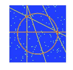
(a) Original image

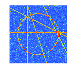
(b) Noisy image

(c) Pointlike Component

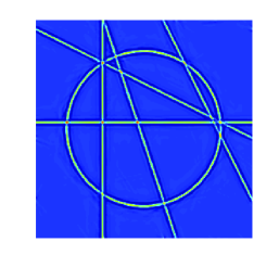
(d) Curvelike Component

Figure 2: Separation of an artificial image composed of points, lines, and a circle into point- and curvelike components using ShearLab.

For illustrative purposes, Figure 2 shows the separation of an artificial image composed of points, lines, and a circle as well as added noise into the pointlike structures (points) and the curvelike structures (lines and the circle), while removing the noise simultaneously. The only visible artifacts can be seen at the intersections of the curvelike structures, which is not surprising since it is even justifiable to label these intersections as ‘points’. As an example using real data, we present in Figure 3 the separation of a neuron image into dendrites and spines again using ShearLab.

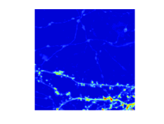
(a) Original image

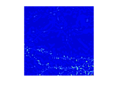
(b) Pointlike Component

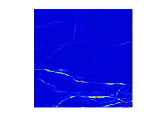
(c) Curvelike Component

Figure 3: Separation of a neuron image into point- and curvelike components using ShearLab.

Another widely explored category of image separation is the separation of cartoons and texture. Here, the term cartoon typically refers to a piecewise smooth part in the image, and texture means a periodic structure. A mathematical model for a cartoon was first introduced in [8] as a $C^{2}$ function containing a $C^{2}$ discontinuity. In contrast to this, the term texture is a widely open expression, and people have debated for years over an appropriate model for the texture content of an image. A viewpoint from applied harmonic analysis characterizes texture as a structure which exhibits a sparse expansion in a Gabor system. As a side remark, the reader should be aware that periodizing a cartoon part of an image produces a texture component, thereby revealing the very fine line between cartoons and texture, illustrated in Figure 4.

Figure 4: Periodic small cartoons versus one large cartoon.

As sparsifying systems, again curvelets or shearlets are suitable for the cartoon part, whereas discrete cosines or a Gabor system can be used for the texture part. MCALab uses for this separation task a dictionary composed of curvelets and discrete cosines, see [35]. For illustrative purposes, we display in Figure 5 the separation of the Barbara image into cartoon and texture component performed by MCALab. As can be seen, all periodic structure is captured in the texture part, leaving the remainder to the cartoon component.

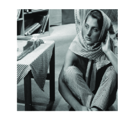
(a) Barbara image

(b) Cartoon Component

(c) Texture Component

Figure 5: Separation of the Barbara image into cartoon and texture using MCALab.

4.2 Theoretical Results

The first theoretical result explaining the successful empirical performance of Morphological Component Analysis was derived in [14] by considering the separation of point- and curvelike features in images coined the Geometric Separation Problem. The analysis in this paper has three interesting features. Firstly, it introduces the notion of cluster coherence (cf. Definition 2.8) as a measure for the geometric arrangements of the significant coefficients and hence the encoding of the morphological difference of the components. It also initiates the study of $\ell_{1}$ minimization in frame settings, in particular those where singleton coherence within one frame may be high. Secondly, it provides the first analysis of a continuum model in contrast to the previously studied discrete models which obscure continuum elements of geometry. And thirdly, it explores microlocal analysis to understand heuristically why separation might be possible and to organize a rigorous analysis. This general approach applies in particular to two variants of geometric separation algorithms. One is based on tight frames of radial wavelets and curvelets and the other uses orthonormal wavelets and shearlets.

These results are today the only results providing a theoretical foundation to image separation using ideas from sparsity methodologies. The same situation – separating point- and curvelike objects – is also considered in [13] however using thresholding as a separation technique. Finally, we wish to mention that some initial theoretical results on the separation of cartoon and texture in images are contained in [15].

Let us now dive into the analysis of [14]. As a mathematical model for a composition of point- and curvelike structures, the following two components are considered: The function ${\mathcal{P}}$ on $\mathbb{R}^{2}$, which is smooth except for point singularities and defined by

$${\mathcal{P}}=\sum_{i=1}^{P}|x-x_{i}|^{-3/2},$$

serves as a model for the pointlike objects, and the distribution ${\mathcal{C}}$ with singularity along a closed curve $\tau:[0,1]\rightarrow\mathbb{R}^{2}$ defined by

$${\mathcal{C}}=\int\delta_{\tau(t)}dt,$$

models the curvelike objects. The general model for the considered situation is then the sum of both, i.e.,

$$f={\mathcal{P}}+{\mathcal{C}},$$ (15)

and the Geometric Separation Problem consists of recovering ${\mathcal{P}}$ and ${\mathcal{C}}$ from the observed signal $f$.

As discussed before, one possibility is to set up the minimization problem using an overcomplete system composed of wavelets and curvelets. For the analysis, radial wavelets are used due to the fact that they provide the same subbands as curvelets. To be more precise, let $W$ be an appropriate window function. Then radial wavelets at scale $j$ and spatial position $k=(k_{1},k_{2})$ are defined by the Fourier transforms

$$\hat{\psi}_{\lambda}(\xi)=2^{-j}\cdot W(|\xi|/2^{j})\cdot e^{i\langle k,\xi/2^{j}\rangle},$$

where $\lambda=(j,k)$ indexes scale and position. For the same window function $W$ and a ‘bump function’ $V$, curvelets at scale $j$, orientation $\ell$, and spatial position $k=(k_{1},k_{2})$ are defined by the Fourier transforms

$$\hat{\gamma}_{\eta}(\xi)=2^{-j\frac{3}{4}}\cdot W(|\xi|/2^{j})V((\omega-\theta_{j,\ell})2^{j/2})\cdot e^{i(R_{\theta_{j,\ell}}A_{2^{-j}}k)^{\prime}\xi},$$

where $\theta_{j,\ell}=2\pi\ell/2^{j/2}$, $R_{\theta}$ is planar rotation by $-\theta$ radians, $A_{a}$ is anisotropic scaling with diagonal $(a,\sqrt{a})$, and we let $\eta=(j,\ell,k)$ index scale, orientation, and scale; see [5] for more details. The tiling of the frequency domain generated by these two systems is illustrated in Figure 6.

                      

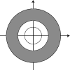
(a) Radial wavelets

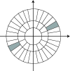
(b) Curvelets

Figure 6: Tiling of the frequency domain by radial wavelets and curvelets.

By using again the window $W$, we define the family of filters $F_{j}$ by their transfer functions

$$\hat{F}_{j}(\xi)=W(|\xi|/2^{j}),\qquad\xi\in\mathbb{R}^{2}.$$

These filters provide a decomposition of any distribution $g$ into pieces $g_{j}$ with different scales, the piece $g_{j}$ at subband $j$ generated by filtering $g$ using $F_{j}$:

$$g_{j}=F_{j}\star g.$$

A proper choice of $W$ then enables reconstruction of $g$ from these pieces using the formula

$$g=\sum_{j}F_{j}\star g_{j}.$$

Application of this filtering procedure to the model image $f$ from (15) yields the decompositions

$$f_{j}=F_{j}\star f=F_{j}\star({\mathcal{P}}+{\mathcal{C}})={\mathcal{P}}_{j}+{\mathcal{C}}_{j},$$

where $(f_{j})_{j}$ is known, and we aim to extract $({\mathcal{P}}_{j})_{j}$ and $({\mathcal{C}}_{j})_{j}$. We should mention at this point that, in fact, the pair $({\mathcal{P}},{\mathcal{C}})$ was chosen in such a way that ${\mathcal{P}}_{j}$ and ${\mathcal{C}}_{j}$ have the same energy for each $j$, thereby making the components comparable as we go to finer scales and the separation challenging at each scale.

Let now $\Phi_{1}$ and $\Phi_{2}$ be the tight frame of radial wavelets and curvelets, respectively. Then, for each scale $j$, we consider the $\ell_{1}$ minimization problem $(\mbox{Sep}_{a})$ stated in (6), which now reads:

$$\min_{P_{j},C_{j}}\|\Phi^{T}_{1}P_{j}\|_{1}+\|\Phi^{T}_{2}C_{j}\|_{1}\quad\textrm{s.t.}\quad f_{j}=P_{j}+C_{j}.$$ (16)

Notice that we use the ‘analysis version’ of the minimization problem, since both radial wavelets as well as curvelets are overcomplete systems.

The theoretical result of the precision of separation of $f_{j}$ via (16) proved in [14] can now be stated in the following way:

Theorem 4.1 ([14])

Let $\hat{P}_{j}$ and $\hat{C}_{j}$ be the solutions to the optimization problem (16) for each scale $j$. Then we have

$$\frac{\|{\mathcal{P}}_{j}-\hat{P}_{j}\|_{2}+\|{\mathcal{C}}_{j}-\hat{C}_{j}\|_{2}}{\|{\mathcal{P}}_{j}\|_{2}+\|{\mathcal{C}}_{j}\|_{2}}\rightarrow 0,\quad j\rightarrow\infty.$$

This result shows that the components ${\mathcal{P}}_{j}$ and ${\mathcal{C}}_{j}$ are recovered with asymptotically arbitrarily high precision at very fine scales. The energy in the pointlike component is completely captured by the wavelet coefficients, and the curvelike component is completely contained in the curvelet coefficients. Thus, the theory evidences that the Geometric Separation Problem can be satisfactorily solved by using a combined dictionary of wavelets and curvelets and an appropriate $\ell_{1}$ minimization problem, as already the empirical results indicate.

We next provide a sketch of proof and refer to [14] for the complete proof.

Proof [Sketch of proof of Theorem 4.1]. The main goal will be to apply Theorem 2.12 to each scale and prove that the sequence of bounds $\frac{2\delta}{1-2\mu_{c}}$ converges to zero. For this, let $j$ be arbitrarily fixed, and apply Theorem 2.12 in the following way:

• $S$: Filtered signal $f_{j}$ $(={\mathcal{P}}_{j}+{\mathcal{C}}_{j})$.

• $\Phi_{1}$: Wavelets filtered with $F_{j}$.

• $\Phi_{2}$: Curvelets filtered with $F_{j}$.

• $\Lambda_{1}$: Significant wavelet coefficients of ${\mathcal{P}}_{j}$.

• $\Lambda_{2}$: Significant curvelet coefficients of ${\mathcal{C}}_{j}$.

• $\delta_{j}$: Degree of approximation by significant coefficients.

• $(\mu_{c})_{j}$: Cluster coherence of wavelets-curvelets.

If

$$\frac{2\delta_{j}}{1-2(\mu_{c})_{j}}=o(\|{\mathcal{P}}_{j}\|_{2}+\|{\mathcal{C}}_{j}\|_{2})\quad\mbox{as }j\to\infty$$ (17)

can be then shown, the theorem is proved.

One main problem to overcome is the highly delicate choice of $\Lambda_{1}$ and $\Lambda_{2}$. It would be ideal to define those sets in such a way that

$$\delta_{j}=o(\|{\mathcal{P}}_{j}\|_{2}+\|{\mathcal{C}}_{j}\|_{2})\quad\mbox{as }j\to\infty$$ (18)

and

$$(\mu_{c})_{j}\to 0\quad\mbox{as }j\to\infty$$ (19)

are true. This would then imply (17), hence finish the proof.

A microlocal analysis viewpoint now provides insight into how to suitably choose $\Lambda_{1}$ and $\Lambda_{2}$ by considering the wavefront sets of ${\mathcal{P}}$ and ${\mathcal{C}}$ in phase space $\mathbb{R}^{2}\times[0,2\pi)$, i.e.,

$$WF({\mathcal{P}})=\{x_{i}\}_{i=1}^{P}\times[0,2\pi)$$

and

$$WF({\mathcal{C}})=\{(\tau(t),\theta(t)):t\in[0,L(\tau)]\},$$

where $\tau(t)$ is a unit-speed parametrization of $\tau$ and $\theta(t)$ is the normal direction to $\tau$ at $\tau(t)$. Heuristically, the significant wavelet coefficients should be associated with wavelets whose index set is ‘close’ to $WF({\mathcal{P}})$ in phase space and, similarly, the significant curvelet coefficients should be associated with curvelets whose index set is ‘close’ to $WF({\mathcal{C}})$. Thus, using Hart Smith’s phase space metric,

$$d_{HS}((b,\theta);(b^{\prime},\theta^{\prime})) = |\langle e_{\theta},b-b^{\prime}\rangle|+|\langle e_{\theta^{\prime}},b-b^{\prime}\rangle|+|b-b^{\prime}|^{2}+|\theta-\theta^{\prime}|^{2},$$

where $e_{\theta}=(\cos(\theta),\sin(\theta))$, an ‘approximate’ form of sets of significant wavelet coefficients is

$$\Lambda_{1,j}=\{\mbox{wavelet lattice}\}\cap\{(b,\theta):d_{HS}((b,\theta);WF({\mathcal{P}}))\leq\eta_{j}2^{-j}\},$$

and an ‘approximate’ form of sets of significant curvelet coefficients is

$$\Lambda_{2,j}=\{\mbox{curvelet lattice}\}\cap\{(b,\theta):d_{HS}((b,\theta);WF({\mathcal{C}}))\leq\eta_{j}2^{-j}\}$$

with a suitable choice of the distance parameters $(\eta_{j})_{j}$. In the proof of Theorem 4.1, the definition of $(\Lambda_{1,j})_{j}$ and $(\Lambda_{2,j})_{j}$ is much more delicate, but follows this intuition. Lengthy and technical estimates then lead to (18) and (19), which – as mentioned before – completes the proof. $\Box$

Since it was already mentioned in Subsection 4.1 that a combined dictionary of wavelets and shearlets might be preferable, the reader will wonder whether the just discussed theoretical results can be transferred to this setting. In fact, this is proven in [26], see also [12]. It should be mentioned that one further advantage of this setting is the fact that now a basis of wavelets can be utilized in contrast to the tight frame of radial wavelets explored before.

As a wavelet basis, we now choose orthonormal Meyer wavelets, and refer to [30] for the definition. For the definition of shearlets, for $j\geq 0$ and $k\in\mathbb{Z}$, let – the notion $A_{2^{j}}$ was already introduced in the definition of curvelets – $\tilde{A}_{2^{j}}$ and $S_{k}$ be defined by

$$\tilde{A}_{2^{j}}=\begin{pmatrix}2^{j/2}&0\\ 0&2^{j}\end{pmatrix}\quad\text{and}\quad S_{k}=\begin{pmatrix}1&k\\ 0&1\end{pmatrix}.$$

For $\phi,\psi,\tilde{\psi}\in L^{2}({\mathbb{R}}^{2})$, the cone-adapted discrete shearlet system is then the union of

$$\{\phi(\cdot-m):m\in{\mathbb{Z}}^{2}\},$$

$$\{2^{\frac{3}{4}j}\psi(S_{k}A_{2^{j}}\,\cdot\,-m):j\geq 0,-\lceil 2^{j/2}\rceil\leq k\leq\lceil 2^{j/2}\rceil,m\in{\mathbb{Z}}^{2}\},$$

and

$$\{2^{\frac{3}{4}j}\tilde{\psi}(S^{T}_{k}\tilde{A}_{2^{j}}\,\cdot\,-m):j\geq 0,-\lceil 2^{j/2}\rceil\leq k\leq\lceil 2^{j/2}\rceil,m\in{\mathbb{Z}}^{2}\}.$$

The term ‘cone-adapted’ originates from the fact that these systems tile the frequency domain in a cone-like fashion; see Figure 7b.

                      

(a) Wavelets

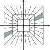
(b) Shearlets

Figure 7: Tiling of the frequency domain by orthonormal Meyer wavelets and shearlets.

As can be seen from Figure 7, the subbands associated with orthonormal Meyer wavelets and shearlets are the same. Hence a similar filtering into scaling subbands can be performed as for radial wavelets and curvelets.

Adapting the optimization problem (16) by using wavelets and shearlets instead of radial wavelets and curvelets generates purported point- and curvelike objects $\hat{W}_{j}$ and $\hat{S}_{j}$, say, for each scale $j$. Then the following result, which shows similarly successful separation as Theorem 4.1, was derived in [26] with the new concept of sparsity equivalence, here between shearlets and curvelets, introduced in the same paper as main ingredient.

Theorem 4.2 ([26])

We have

$$\frac{\|{\mathcal{P}}_{j}-\hat{W}_{j}\|_{2}+\|{\mathcal{C}}_{j}-\hat{S}_{j}\|_{2}}{\|{\mathcal{P}}_{j}\|_{2}+\|{\mathcal{C}}_{j}\|_{2}}\rightarrow 0,\quad j\rightarrow\infty.$$

References

- [1] Aharon, M., Elad, M., and Bruckstein, A.M. (2006). The K-SVD: An algorithm for designing of overcomplete dictionaries for sparse representation, IEEE Trans. Signal Proc., 54(11), 4311–4322.
- [2] Bobin, J., Starck, J.-L., Fadili, M.J., Moudden, Y., and Donoho, D.L. (2007). Morphological component analysis: An adaptive thresholding strategy, IEEE Trans. Image Proc., 16(11), 2675–2681.
- [3] Borup, L., Gribonval, R., and Nielsen, M. (2008). Beyond coherence: Recovering structured time-frequency representations, Appl. Comput. Harmon. Anal., 24(1), 120–128.
- [4] Bruckstein, A.M., Donoho, D.L., and Elad, M. (2009). From sparse solutions of systems of equations to sparse modeling of signals and images, SIAM Review, 51(1), 34–81.
- [5] Candès, E.J. and Donoho, D.L. (2005). Continuous curvelet transform: II. Discretization of frames, Appl. Comput. Harmon. Anal., 19(2), 198–222.
- [6] Chen, S. S., Donoho, D. L., and Saunders, M. A. (1998). Atomic decomposition by basis pursuit, SIAM J. Sci. Comput., 20(1), 33–61.
- [7] Coifman, R.R. and Wickerhauser, M.V. (1993). Wavelets and adapted waveform analysis. A toolkit for signal processing and numerical analysis, Different perspectives on wavelets (San Antonio, TX, 1993), 119–153, Proc. Sympos. Appl. Math., 47, Amer. Math. Soc., Providence, RI.
- [8] Donoho, D.L. (2001). Sparse components of images and optimal atomic decomposition, Constr. Approx., 17(3), 353–382.
- [9] Donoho, D.L. (2006). Compressed sensing, IEEE Trans. Inform. Theory, 52(4), 1289–1306.
- [10] Donoho, D.L. and Elad, M. (2003). Optimally sparse representation in general (nonorthogonal) dictionaries via minimization, Proc. Natl. Acad. Sci. USA, 100(5), 2197–2202.
- [11] Donoho, D.L. and Huo, X. (2001). Uncertainty principles and ideal atomic decomposition, IEEE Trans. Inform. Theory, 47(7), 2845–2862.
- [12] Donoho, D.L. and Kutyniok, G. (2009). Geometric separation using a wavelet-shearlet dictionary, SampTA’09 (Marseille, France, 2009), Proc., 2009.
- [13] Donoho, D.L. and Kutyniok, G. (2010). Geometric separation by single-pass alternating thresholding, preprint.
- [14] Donoho, D.L. and Kutyniok, G. (2010). Microlocal analysis of the geometric separation problem, preprint.
- [15] Donoho, D.L. and Kutyniok, G. (2011). Geometric separation of cartoons and texture via minimization, preprint.
- [16] Donoho, D.L. and Stark, P.B. (1989). Uncertainty principles and signal recovery, SIAM J. Appl. Math., 49(3), 906–931.
- [17] Duarte-Carvajalino, J.M. and Sapiro, G. (2009). Learning to sense sparse signals: Simultaneous sensing matrix and sparsifying dictionary optimization, IEEE Trans. Image Proc., 18(7), 1395–1408.
- [18] Elad, M. (2010). Sparse and redundant representations, Springer, New York.
- [19] Elad, M. and Bruckstein, A. M. (2002). A generalized uncertainty principle and sparse representation in pairs of bases, IEEE Trans. Inform. Theory, 48(9), 2558–2567.
- [20] Elad, M., Starck, J.-L., Querre, P., and Donoho, D.L. (2005). Simultaneous cartoon and texture image inpainting using morphological component analysis (MCA), Appl. Comput. Harmon. Anal., 19(3), 340–358.
- [21] Engan, K., Aase, S.O., and Hakon-Husoy, J.H. (1999). Method of optimal directions for frame design, IEEE Int. Conf. Acoust., Speech, Signal Process., 5, 2443- 2446.
- [22] Gribonval, R. and Bacry, E. (2003). Harmonic decomposition of audio signals with matching pursuit, IEEE Trans. Signal Proc., 51(1), 101–111.
- [23] Gribonval, R. and Nielsen, M. (2003). Sparse representations in unions of bases, IEEE Trans. Inform. Theory, 49(12), 3320–3325.
- [24] Guo, K., Kutyniok, G., and Labate, D. (2006). Sparse multidimensional representations using anisotropic dilation and shear operators, Wavelets and Splines (Athens, GA, 2005), Nashboro Press, Nashville, TN, 2006, 189–201.
- [25] Kowalski, M. and Torrésani, B. (2010). Sparsity and persistence: Mixed norms provide simple signal models with dependent coefficients, Signal, Image and Video Proc., to appear.
- [26] Kutyniok, G. (2010). Sparsity equivalence of anisotropic decompositions, preprint.
- [27] Kutyniok, G., Lemvig, J., and Lim, W.-Q (2010). Compactly supported shearlets, Approximation Theory XIII (San Antonio, TX, 2010), Springer, to appear.
- [28] Kutyniok, G. and Lim, W.-Q (2010). Compactly supported shearlets are optimally sparse, preprint.
- [29] Kutyniok, G. and Lim, W.-Q (2010). Image separation using shearlets, preprint.
- [30] Mallat, S.G. (1998). A wavelet tour of signal processing, Academic Press, Inc., San Diego, CA.
- [31] Mallat, S.G. and Zhang, Z. (1993). Matching pursuits with time-frequency dictionaries, IEEE Trans. Signal Proc., 41(12), 3397–3415.
- [32] Meyer, F.G., Averbuch, A., and Coifman, R.R. (2002). Multi-layered image representation: Application to image compression, IEEE Trans. Image Proc., 11(9), 1072–1080.
- [33] Starck, J.-L., Murtagh, F., and Fadili, J.M. (2010). Sparse Image and Signal Processing: Wavelets, Curvelets, Morphological Diversity, Cambridge University Press, New York, NY.
- [34] Starck, J.-L., Elad, M., and Donoho, D.L. (2005). Redundant multiscale transforms and their application for morphological component analysis, Adv. Imag. Electr. Phys., 132, 287–348.
- [35] Starck, J.-L., Elad, M., and Donoho, D.L. (2005). Image decomposition via the combination of sparse representations and a variational approach, IEEE Trans. Image Proc., 14(10), 1570–1582.
- [36] Starck, J.-L., Moudden, Y., Bobin, J., Elad, M., and Donoho, D.L. (2005). Morphological component analysis, Wavelets XI (San Diego, CA, 2005), SPIE Proc. 5914, SPIE, Bellingham, WA.
- [37] Tropp, J.A. (2004). Greed is good: Algorithmic results for sparse approximation, IEEE Trans. Inform. Theory, 50(10), 2231–2242.
- [38] Tropp, J.A. (2008). On the linear independence of spikes and sines, J. Fourier Anal. Appl., 14(5-6), 838–858.
- [39] Tropp, J.A. (2010). The sparsity gap: Uncertainty principles proportional to dimension, Proc. 44th IEEE Conf. Information Sciences and Systems (CISS), 1–6, Princeton, NJ.