Entropy-driven cutoff phenomena

Abstract

In this paper we present, in the context of Diaconis’ paradigm, a general method to detect the cutoff phenomenon. We use this method to prove cutoff in a variety of models, some already known and others not yet appeared in literature, including a chain which is non-reversible w.r.t. its stationary measure. All the given examples clearly indicate that a drift towards the opportune quantiles of the stationary measure could be held responsible for this phenomenon. In the case of birth-and-death chains this mechanism is fairly well understood; our work is an effort to generalize this picture to more general systems, such as systems having stationary measure spread over the whole state space or systems in which the study of the cutoff may not be reduced to a one-dimensional problem. In those situations the drift may be looked for by means of a suitable partitioning of the state space into classes; using a statistical mechanics language it is then possible to set up a kind of energy-entropy competition between the weight and the size of the classes. Under the lens of this partitioning one can focus the mentioned drift and prove cutoff with relative ease.

Keywords: Finite Markov chains, hitting times, cutoff, random walk on the hypercube.

1 Introduction and Main Results

In this paper we present sufficient conditions for a family of finite ergodic Markov chains to exhibit cutoff. Roughly speaking the cutoff phenomenon is an abrupt convergence of a Markov chain to its equilibrium distribution. The detailed description of the cutoff phenomenon is given by means of two quantities, the cutoff-time and the cutoff-window, the latter being much smaller than the former. For an overview on the cutoff phenomenon we refer the reader to the review paper by Diaconis [9] and the book by Levin, Peres and Wilmer [6].

Our main results, Theorem 1.2 and its corollary, identify with much clarity the cutoff-time as the expected value of a certain hitting time, and for the first time in literature such hitting time is related to some entropy considerations, see Section 1.2 below. Corollary 1.3 also gives evidence of the nature of the cutoff-window, which is in turn kindred to the standard deviation of the hitting time mentioned above and/or to the mixing features of the chain. The level of generality of the key results gives the possibility to use statistical-mechanics-based ideas to prove cutoff for a variety of models known in literature, such as Coupon Collector, Top-in-at-random, Ehrenfest Urn, Random walk on the hypercube and mean-field Ising model. Furthermore, we prove cutoff for a couple of one-parameter families of random walks, partially biased (i.e. with drift) and partially diffusive, whose peculiar feature is to have cutoff-window of different order depending on the parameter. It is worthy to notice that the first of those families is an example of non-reversible chain exhibiting cutoff (see Section 3.4).

Section 1.1 defines the structure of our study, Section 1.2 gives some of the ideas standing behind the main results and draw a comparison with previous approaches. Section 1.3 states our key theorems while Section 1.4 examines them and gives an explanation of the hypothesis. All the proofs are deferred to Section 2. In Section 3 we discuss the application of our results to the models mentioned above.

1.1 Framework and notation

In what follows we will consider families of finite ergodic Markov chains, that is sextets of the form

$$\{\Omega_{n},X_{n}^{t},P_{n},\pi_{n},\mu_{n}^{t},\mu_{n}^{0}\}$$

where $\Omega_{n}$ is the finite state space of the $n$-th chain, $X_{n}^{t}$, which has transition matrix $P_{n}$ and unique stationary measure $\pi_{n}$. The symbols $\mu_{n}^{0}$ and $\mu_{n}^{t}$ stand for the initial distribution of the $n$-th chain and its probability distribution after $t$ steps. The time $t$ is a discrete quantity. For brevity we will refer to such families simply as families of Markov chains, omitting the expression “finite ergodic” throughout the whole paper.

Definition 1.1.

A family of Markov chains is said to exhibit cutoff if there exist two sequences of integers, $\{a_{n}\}$ and $\{b_{n}\}$ such that

$$\frac{b_{n}}{a_{n}}\TendsTo[n,\infty]0$$ (1.1)

and

$$\lim_{\theta\to\infty}\liminf_{n\to\infty}d_{\text{\tiny TV}}\left(\mu_{n}^{a_{n}-\theta b_{n}},\pi_{n}\right) =1$$ (1.2)

$$\lim_{\theta\to\infty}\limsup_{n\to\infty}d_{\text{\tiny TV}}\left(\mu_{n}^{a_{n}+\theta b_{n}},\pi_{n}\right) =0$$ (1.3)

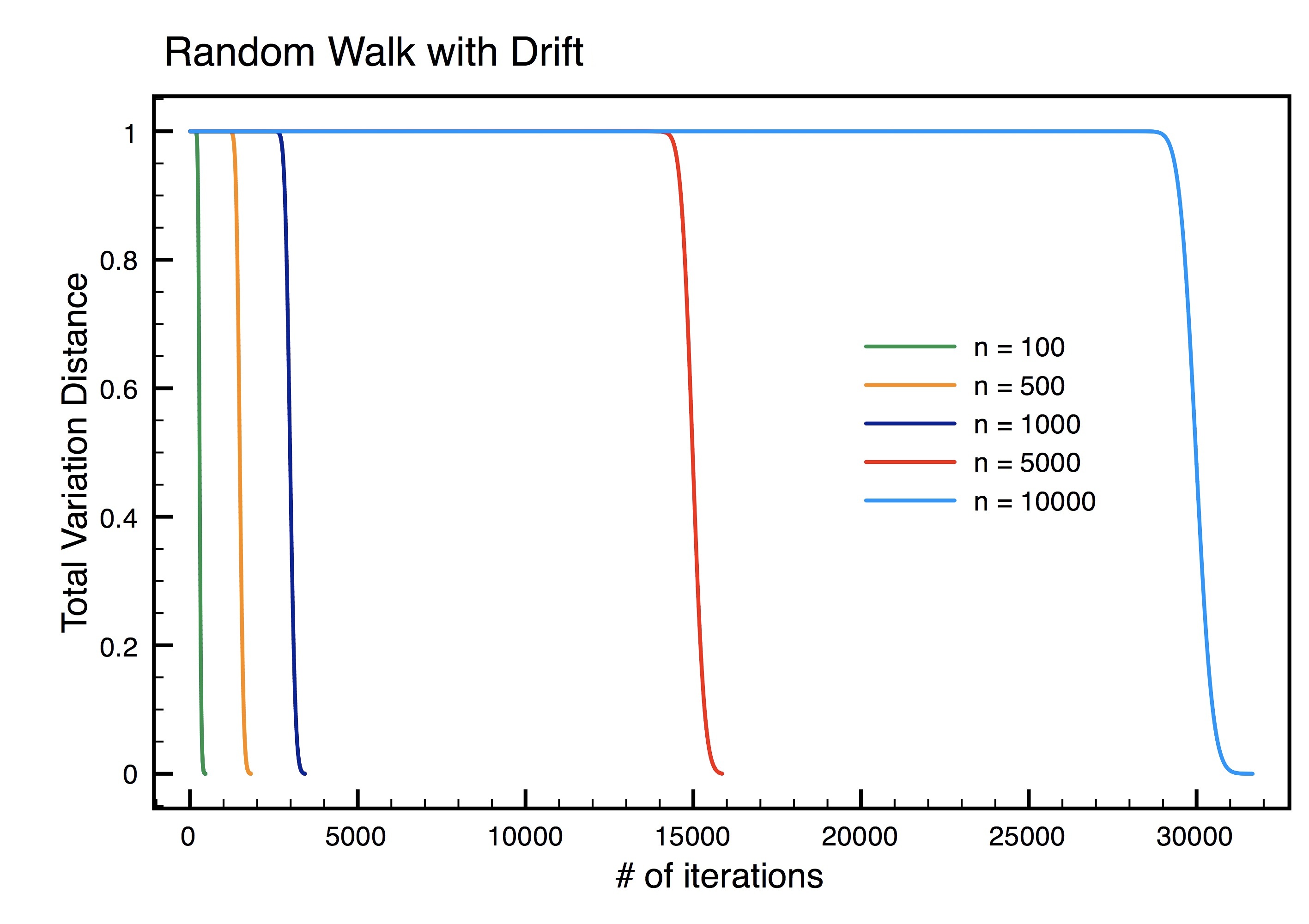
Figure 1: Biased random walk on a segment. The transition probabilities are $P_{i,i-1}=\frac{1}{6}$, $P_{i,i}=\frac{1}{3}$ and $P_{i,i+1}=\frac{1}{2}$. The curves refer to different values of $n$, the length of the segment.

Equations (1.2) and (1.3) represent the sharp convergence to the equilibrium distribution, see Figure 1. The distance from stationarity is taken here to be the usual total variation distance

$$d_{\text{\tiny TV}}\left(\mu_{n}^{t},\pi_{n}\right) =\frac{1}{2}\sum_{i\in\Omega_{n}}\left|\pi_{n}(i)-\mu_{n}^{t}(i)\right|=\max_{A\in\Omega_{n}}\left[\pi_{n}(A)-\mu_{n}^{t}(A)\right]$$ (1.4)

Remark 1.1.

Definition 1.1 was first introduced in [12]. Although there exist equivalent alternative definitions of cutoff (see [3], [1] and [8]) we prefer to work with the one given, for it leaves us control on the cutoff-window.

As mentioned above there exists a connection between the cutoff-time and the expectation of an hitting time. That connection can be easily pointed out if we think of the total variation distance between $\mu_{n}^{t}$ and $\pi_{n}$ (which, in principle, could be computed at any given time) as a random variable, or better as a deterministic object computed at a stochastic time. This idea motivates the following

Definition 1.2.

Given a random variable $\xi$, we define the total variation distance at time $\xi$ as the following r.v.

$$d_{\text{\tiny TV}}\left(\mu_{n}^{\xi},\pi_{n}\right)=\sum_{t\in\mathbb{Z}}d_{\text{\tiny TV}}\left(\mu_{n}^{t_{+}},\pi_{n}\right)\mathds{1}_{\{\xi=t\}}$$ (1.5)

where $t_{+}=\max\{0,t\}$. When $\xi$ takes values in $[-a,+\infty)$, with $a\in\mathbb{R}^{+}$, this definition is equivalent to

$$d_{\text{\tiny TV}}\left(\mu_{n}^{\xi},\pi_{n}\right) =\sum_{t\geq-a}\left[d_{\text{\tiny TV}}\left(\mu_{n}^{t},\pi_{n}\right)\mathds{1}_{\{\xi=t,\,\xi\geq 0\}}+d_{\text{\tiny TV}}\left(\mu_{n}^{0},\pi_{n}\right)\mathds{1}_{\{\xi=t,\,\xi<0\}}\right]$$ (1.5a)

We need this definition because in the statements of the key theorems we will consider the expectation of (1.5a) at the stochastic time $\zeta-a$, where $\zeta\geq 0$ is a hitting time. This is a natural consequence of our aim to care about the cutoff-window. The expectation of (1.5a) can be computed as

$$\mathbb{E}\left[d_{\text{\tiny TV}}\left(\mu_{n}^{\xi},\pi_{n}\right)\right] =\sum_{t\geq 0}d_{\text{\tiny TV}}\left(\mu_{n}^{t},\pi_{n}\right)\mathbb{P}\left(\xi=t,\,\xi\geq 0\right)+d_{\text{\tiny TV}}\left(\mu_{n}^{0},\pi_{n}\right)\mathbb{P}\left(\xi<0\right)$$ (1.6)

Although the condition $\xi\geq 0$ could be dropped in the first sum of (1.6), we prefer to keep it for notational purposes that will become clear in the proof of Theorem 1.2.

1.2 Cutoff-times and hitting-times

Theorem 1.2 and its Corollary 1.3 bring to light the link between the cutoff phenomenon and the hitting of the relevant part of the state space $\Omega_{n}$. Relevant part means the subset of the state space where the stationary distribution $\pi_{n}$ is mostly concentrated, see equation (1.16) below. This seems quite a natural approach when we realize that nearly every chain known to exhibit cutoff hits the relevant part of the state space in a quasi-deterministic way, that is the hitting time $\tau_{n}$ of such a relevant part satisfies the following limit:

$$\frac{\sigma\left[\tau_{n}\right]}{\mathbb{E}\left[\tau_{n}\right]}\TendsTo[n,\infty]0$$ (1.7)

where $\sigma\left[\tau_{n}\right]$ is the standard deviation of $\tau_{n}$. It is relatively easy to prove a limit as in (1.7) whenever the chain presents a drift towards the relevant part of the state space. In Section 3 we present a rich selection of examples of applications of our theorems as well as a comparison with the existing literature.

The picture of a quasi-deterministic hitting we have described so far holds as well for the systems with uniform stationary measure, for which the relevant part of the state space would be $\Omega_{n}$ itself. As a matter of fact, if we desist from the whole description of such a chain and look into a suitable projection, then we may find that the original stationary distribution is no longer uniform. The projected stationary distribution, $\nu_{n}(x)$, is indeed proportional to the number of states $i\in\Omega_{n}$ which correspond to $x$ according to the equivalence relation we used to project the original chain. Consequently, since $-\nu_{n}(x)\log\nu_{n}(x)$ is the contribution to the entropy of $\nu_{n}$ given by the $x$-th equivalence class, we have that the relevant part of the state space is composed of the classes providing the leading contribution to the entropy. In these cases the drift mentioned above is therefore supplied by entropic considerations; we will return to this point later on in Section 3. With respect to what we have said above, Corollary 1.3 represents then a possible trait d’union between two classes of Markov chains exhibiting cutoff: the first being made up of chains having stationary measure concentrated in a small subset of the state space, like birth-and-death chains with drift, and the second composed of those chains with stationary measure uniform or spread over $\Omega_{n}$, like the random walk on the hypercube, many card-shuffling models and some high-temperature statistical mechanics models.

The idea of relating cutoff with the hitting of the appropriate quantiles of the stationary distribution is already present in literature, see [1], [5], [8] and [3]. In [1] and [5] the cutoff is completely characterized for the special case of birth-and-death chains, respectively in total variation and in separation distance. A discussion of the results in [1] is deferred to Section 1.4 after we have stated our main theorems. With respect to [8] and [3] our approach allows the study of the cutoff phenomena in a context closer to the classical Diaconis’ paradigm. In particular, with respect to the former reference we define cutoff in a finite configurations space and consequently we have a precise control of the cutoff-window. With respect to the latter, we will show in Sections 1.4 and 3.5 that our tackle to the problem produces a clearer understanding of the role of the drift in the cutoff phenomena.

1.3 Key results

In this first theorem, that will be the main ingredient of the proof of Theorem 1.2, we relate the cutoff phenomenon to systems having an abrupt convergence to equilibrium at a stochastic time which is quasi-deterministic in the sense of (1.7).

Theorem 1.1.

Let $\{\Omega_{n},X_{n}^{t},P_{n},\pi_{n},\mu_{n}^{t},\mu_{n}^{0}\}$ a family of Markov chains, $\{\tau_{n}\}$ a family of non-negative random variables with finite expected value $E_{n}=\mathbb{E}\left[\tau_{n}\right]$ and standard deviation $\sigma_{n}=\sigma\left[\tau_{n}\right]$ such that

$$\lim_{n\to\infty}\frac{\sigma_{n}}{E_{n}}=0$$ (1.8)

Let $\{\delta_{n}\}$ be a sequence of positive numbers such that

$$\lim_{n\to\infty}\frac{\delta_{n}}{E_{n}}=0$$ (1.9)

$$\text{definitively for }n\to\infty \quad\mathbb{E}\left[d_{\text{\tiny TV}}\left(\mu_{n}^{\tau_{n}-\theta\delta_{n}},\pi_{n}\right)\right]\geq 1-f(\theta)$$ (1.10)

$$\text{definitively for }n\to\infty \quad\mathbb{E}\left[d_{\text{\tiny TV}}\left(\mu_{n}^{\tau_{n}+\theta\delta_{n}},\pi_{n}\right)\right]\leq g(\theta)$$ (1.11)

where $f$ and $g$ are two functions tending to $0$ as $\theta\to\infty$.

Then the family exhibits cutoff with

$$a_{n} =E_{n}$$ (1.12)

$$b_{n} =O(\sigma_{n}+\delta_{n})$$ (1.13)

Before we move to the statement of Theorem 1.2 we need to introduce some tools.

Definition 1.3.

We define a family of nested subsets as a sequence $\{A_{n,\theta}\}_{\theta\geq 1}$ with the following properties: $\forall\,\theta\in\mathbb{N},\>\>\exists\,N>0\text{ such that }\forall\,n\geq N$

$$A_{n,\theta^{\prime}}\subset\Omega_{n} \forall\,1\leq\theta^{\prime}\leq\theta$$ (1.14)

$$A_{n,\theta^{\prime}}\subseteq A_{n,\theta^{\prime\prime}} \forall\,1\leq\theta^{\prime}\leq\theta^{\prime\prime}\leq\theta$$ (1.15)

Definition 1.4.

Given a family of nested subsets we shall say that $\pi_{n}$ is h-concentrated on $A_{n,\theta}$ if there exists a function $h(\theta)$ tending to zero as $\theta\to\infty$ such that

$$\text{definitively as }n\to\infty\qquad\pi_{n}(A_{n,\theta}^{\complement})<h(\theta)$$ (1.16)

where $A_{n,\theta}^{\complement}=\Omega_{n}\setminus A_{n,\theta}$.

Finally, define $\zeta_{n}^{\theta}=\min\{t\geq 0\,:\,X_{n}^{t}\in A_{n,\theta}\}$ the hitting time of $A_{n,\theta}$; note that $\zeta_{n}^{\theta}\geq\zeta_{n}^{\theta^{\prime}}$ if $\theta\leq\theta^{\prime}$. We are now ready to state the main result of this paper.

Theorem 1.2.

Let $\{\Omega_{n},X_{n}^{t},P_{n},\pi_{n},\mu_{n}^{t},\mu_{n}^{0}\}$ a family of Markov chains. Suppose that $\mu_{n}^{0}$ is such that there exists a family of nested subsets $\{A_{n,\theta}\}_{\theta\geq 1}\subset\Omega_{n}$ with the following properties:

$$\pi_{n}\text{ is h-concentrated in }A_{n,\theta}$$ (1.17)

$$\frac{\sigma\left[\zeta_{n}^{1}\right]}{\mathbb{E}\left[\zeta_{n}^{1}\right]}\TendsTo[n,\infty]0$$ (1.18)

$$\sigma\left[\zeta_{n}^{\theta}\right]\leq\sigma\left[\zeta_{n}^{1}\right]$$ (1.19)

and there exists a sequence of positive integers $\{\Delta_{n}\}$ such that

$$\frac{\Delta_{n}}{\mathbb{E}\left[\zeta_{n}^{1}\right]}\TendsTo[n,\infty]0$$ (1.20)

$$\lim_{\theta\to\infty}\lim_{n\to\infty}\frac{\mathbb{E}\left[\zeta_{n}^{1}-\zeta_{n}^{\theta}\right]}{\theta\Delta_{n}}=0$$ (1.21)

Then there exists a function $f(\theta)$, tending to 0 as $\theta\to\infty$, such that

$$\mathbb{E}\left[d_{\text{\tiny TV}}\left(\mu_{n}^{\zeta_{n}^{1}-\theta\delta_{n}},\pi_{n}\right)\right]\geq 1-f(\theta) \quad\text{definitively for }n\to\infty$$ (1.22)

where

$$\delta_{n}=2\,(\Delta_{n}+\sigma\left[\zeta_{n}^{1}\right])$$ (1.23)

A relatively easy consequence of Theorem 1.2 is the following

Corollary 1.3.

Assume that all the hypothesis of Theorem 1.2 hold for a given family of Markov chains. In addition suppose that given two copies of the $n$-th chain of the family, $Z_{n}^{t}$ and $W_{n}^{t}$, there exists a coupling $(Z_{n}^{t},W_{n}^{t})$ such that

$$Z_{n}^{0}=z_{0}\in A_{n,1}\quad W_{n}^{0}\sim\pi_{n}$$ (1.24)

$$\text{if }Z_{n}^{s^{*}}=W_{n}^{s^{*}}\text{ then }Z_{n}^{s}=W_{n}^{s}\quad\forall\>s\geq s^{*}$$ (1.25)

$$\gamma_{n}=\min\{t\geq 0\>:\>Z_{n}^{t}=W_{n}^{t}\}\text{ is such that }$$

$$\max_{z_{0}\in A_{n,1}}\mathbb{P}\left(\gamma_{n}>\theta\delta_{n}\,|\,Z_{n}^{0}=z_{0}\right)\leq g(\theta)\text{ definitively as }n\to\infty$$ (1.26)

with $g(\theta)\TendsTo[\theta,\infty]0$. Then the family exhibits cutoff with

$$a_{n} =\mathbb{E}\left[\zeta_{n}^{1}\right]$$ (1.27)

$$b_{n} =O(\delta_{n})$$ (1.28)

1.4 Discussion of Theorem 1.2

Theorem 1.2 identifies a general structure that underlies a class of systems exhibiting cutoff: those with stationary measure concentrated in a small region of the state space ($A_{n,\theta}$ in the theorem, see (1.14)-(1.16) above). Although widely general, Theorem 1.2 is most useful when we face a family of Markov chains $X_{n}^{t}$ which is, or can be projected onto, a family of birth-and-death chains. In those cases we have indeed closed formulas to deal with expectation and variance of the various hitting times, see for example [3] or [13]. The non-reversible random walk on a cylindrical lattice, presented in Section 3.4, shows that the application of Theorem 1.2 is not restricted solely to those models where the study of the cutoff can be completely reduced to a one-dimensional problem.

Total variation cutoff was completely settled in [1] for the class of birth-and-death chains, in particular it is shown therein that we have cutoff if and only if $t^{(n)}_{\text{REL}}=o(t^{(n)}_{\text{MIX}})$, where $t^{(n)}_{\text{REL}}$ and $t^{(n)}_{\text{MIX}}$ are respectively the relaxation time and the mixing time of the $n$-th chain. It should be pointed out, however, that in some importat models of statistical mechanics, namely the Ehrenfest urn and the magnetization chain for the mean field Ising model, a non optimal $\sqrt{t^{(n)}_{\text{REL}}\cdot t^{(n)}_{\text{MIX}}}$ window order is found. Our approach conversely, provided a suitable definition of the $A_{n,\theta}$’s (see Remark 1.2 below), is always capable of delivering the right cutoff-window order. Moreover, in most situations the computation of $\mathbb{E}\left[\zeta_{n}^{\theta}\right]$ and $\sigma\left[\zeta_{n}^{\theta}\right]$ happens to be less challenging than the computation of the spectral gap of the chain.

Within the framework of birth-and-death chains, $\pi_{n}$ being concentrated in $A_{n,\theta}$ is equivalent to a drift of the chain towards $A_{n,\theta}$ itself; such a drift is likely to ensure

$$\frac{\sigma\left[\zeta_{n}^{\theta}\right]}{\mathbb{E}\left[\zeta_{n}^{\theta}\right]}\TendsTo[n,\infty]0\qquad\forall\,\theta\geq 1$$ (1.29)

Limit (1.29) means in turn that for $n$ sufficiently large the chain will hit $A_{n,\theta}$ in a quasi-deterministic way, that is the probability of $X_{n}^{t}$ being into $A_{n,\theta}$ will suddenly rise from 0 to 1 in a window of size $\sigma\left[\zeta_{n}^{\theta}\right]$ centered on $\mathbb{E}\left[\zeta_{n}^{\theta}\right]$. This means that, if the system was started outside $A_{n,\theta}$, it is undergoing the first part of the cutoff curve, i.e. it satisfies (1.2). If the system relaxes inside $A_{n,\theta}$ in a time interval that is comparable with $\sigma\left[\zeta_{n}^{\theta}\right]$, then we would experience cutoff with a window of the order of $\sigma\left[\zeta_{n}^{\theta}\right]$. It is also possible that the time $t_{\text{mix}}$ needed for the system to relax inside $A_{n,\theta}$ is larger than $\sigma\left[\zeta_{n}^{\theta}\right]$ but smaller than $\mathbb{E}\left[\zeta_{n}^{\theta}\right]$, implying then cutoff with a cutoff window of the order of $t_{\text{mix}}$. This is the case of the Ehrenfest Urn and the Random Walk on the Hypercube, which we present in detail in Section 3.3.

The technical problem we had to face in designing Theorem 1.2 is the fact that $\mathbb{E}\left[\zeta_{n}^{\theta}\right]$ is not a good candidate to the cutoff-time, $a_{n}$, being $\theta$-dependent. This is the reason why we preferred to split the diffusion inside $A_{n,\theta}$ in two parts: the hitting of $A_{n,1}$, a subset of $\Omega_{n}$ such that $\pi_{n}(A_{n,1})$ is non-vanishing in $n$, and the diffusion time once $A_{n,1}$ is reached, see (1.26).

Remark 1.2.

There is no universal choice for the family $A_{n,\theta}$, multiple definitions are possible and each of them affects indirectly the size of the cutoff-window. Remark 3.8 in Section 3.5 shows a choice for the $A_{n,\theta}$’s which leads to a non optimal cutoff-window. The applications presented in Section 3 also suggest the key to obtain an optimal cutoff-window: design the family $A_{n,\theta}$ in such a way that the expected travelling time $\mathbb{E}\left[\zeta_{n}^{1}-\zeta_{n}^{\theta}\right]$ is of the same order in $n$ as the time $\theta\delta_{n}$ necessary to achieve equilibrium starting anywhere in $A_{n,1}$ (cfr. Corollary 1.3). From the discussion in this section, and in particular from (1.29), we can take an energy-landscape point of view and visualize our system as a single well, where the height of the energy landscape in a given point $i$ increases with $\pi_{n}^{-1}(i)$. Consider for example the Ehrenfest Urn, presented in Section 3.3; requiring that $\mathbb{E}\left[\zeta_{n}^{1}-\zeta_{n}^{\theta}\right]=O(\delta_{n})$ corresponds to say that, once the chain has reached the border of $A_{n,\theta}$, it falls to the bottom of the well (that is $A_{n,1}$) in a time which is also sufficient to diffuse inside the well itself.

Remark 1.3.

Note that, in the case of birth-and-death chains, hypotheses (1.19) is trivial.

Remark 1.4.

We would like to emphasize that the task of showing the cutoff behavior is usually accomplished by means of a coupling argument. In most situations the coupling argument needs to be sufficiently fine, since the desired estimates are to be performed at times $a_{n}\pm\theta b_{n}$, i.e. with two very different time scales involved. In our approach this time scale issue is set loose when we split the study of the cutoff in two phases, namely the hitting of $A_{n,1}$ and the subsequent evolution to equilibrium. We will see later on in the applications (Section 3) that within our framework only very basic and intuitive couplings are demanded.

2 Proof of Main Results

In the following we will make intensively use of two easy and well known facts that are worth of a brief recalling, before we proceed with the proof of the key results.

Lemma 2.1.

(Cantelli’s inequality) Let Y be a random variable with finite mean $\mu$ and finite variance $\sigma^{2}$. Then, for any $\theta\geq 0$

$$\mathbb{P}\left(Y-\mu\geq\theta\sigma\right)\leq\frac{1}{1+\theta^{2}}$$ (2.1)

Lemma 2.2.

Let $X(t)$ be a discrete Markov chain with finite space state. Then the total variation distance from stationarity is a non-increasing sequence as a function of $t$.

A proof of Lemma 2.2 may be found in [7] and a proof of Lemma 2.1 in [14].

Now we can start with the proof of the key results.

Proof of Theorem 1.1.

For brevity of notation set $D(t)\equiv d_{\text{\tiny TV}}\left(\mu_{n}^{t},\pi_{n}\right)$ and $\xi\equiv\tau_{n}-\theta\delta_{n}$; note that according with the latter definition $\mathbb{E}\left[\xi\right]-\theta\sigma_{n}=a_{n}-\theta b_{n}$. Then, using (1.6)

$$\mathbb{E}\left[D(\xi)\right] =\sum_{t\geq 0}D(t)\mathbb{P}\left(\xi=t\,,\,\xi\geq 0\right)+D(0)\mathbb{P}\left(\xi<0\right)$$ (2.2)

$$\leq\sum_{t\geq 0}D(t)\mathbb{P}\left(\xi=t\,,\,\xi\geq 0\right)+\mathbb{P}\left(\xi<0\right)$$ (2.3)

We can estimate the sum in (2.3) as follows

$$\sum_{t\geq 0}D(t)\mathbb{P}\left(\xi=t\,,\,\xi\geq 0\right) \leq\sum_{t=0}^{\mathbb{E}\left[\xi\right]-\theta\sigma_{n}}D(t)\mathbb{P}\left(\xi=t\,,\,\xi\geq 0\right)+$$

$$\qquad\qquad\sum_{t\geq\mathbb{E}\left[\xi\right]-\theta\sigma_{n}}D(t)\mathbb{P}\left(\xi=t\,,\,\xi\geq 0\right)$$ (2.4)

$$\leq\mathbb{P}\left(0\leq\xi\leq\mathbb{E}\left[\xi\right]-\theta\sigma_{n}\right)+D(\mathbb{E}\left[\xi\right]-\theta\sigma_{n})$$ (2.5)

where from (2.4) to (2.5) we have used Lemma 2.2 to estimate the second sum.

Substituting equation (2.5) in (2.3) we obtain

$$\mathbb{E}\left[D(\xi)\right]\leq\mathbb{P}\left(\tau_{n}\leq\mathbb{E}\left[\tau_{n}\right]-\theta\sigma_{n}\right)+D(\mathbb{E}\left[\xi\right]-\theta\sigma_{n})$$ (2.6)

that is

$$\mathbb{E}\left[d_{\text{\tiny TV}}\left(\mu_{n}^{\tau_{n}-\theta\delta_{n}},\pi_{n}\right)\right]\leq d_{\text{\tiny TV}}\left(\mu_{n}^{a_{n}-\theta b_{n}},\pi_{n}\right)+\mathbb{P}\left(\tau_{n}\leq\mathbb{E}\left[\tau_{n}\right]-\theta\sigma_{n}\right)$$ (2.7)

Thus, reverting the inequality, in virtue of (1.10) and (2.1) we arrive at

$$1\geq\liminf_{n\to\infty}d_{\text{\tiny TV}}\left(\mu_{n}^{a_{n}-\theta b_{n}},\pi_{n}\right)\geq 1-f(\theta)-\frac{1}{1+\theta^{2}}$$ (2.8)

Now set $\eta=\tau_{n}+\theta\delta_{n}$ and notice that $\mathbb{E}\left[\eta\right]+\theta\sigma_{n}=a_{n}+\theta b_{n}$. Then since $\eta\geq\theta\delta_{n}$, by (1.6) we get

$$\mathbb{E}\left[D(\eta)\right] =\sum_{t\geq\theta\delta_{n}}D(t)\mathbb{P}\left(t=\eta\right)$$ (2.9)

$$\geq\sum_{t=\theta\delta_{n}}^{\mathbb{E}\left[\eta\right]+\theta\sigma_{n}}D(t)\mathbb{P}\left(t=\eta\right)$$ (2.10)

$$\geq D(\mathbb{E}\left[\eta\right]+\theta\sigma_{n})\sum_{t=\theta\delta_{n}}^{\mathbb{E}\left[\eta\right]+\theta\sigma_{n}}\mathbb{P}\left(t=\eta\right)$$ (2.11)

$$=D(\mathbb{E}\left[\eta\right]+\theta\sigma_{n})\mathbb{P}\left(\eta\leq\mathbb{E}\left[\eta\right]+\theta\sigma_{n}\right)$$ (2.12)

$$\geq D(\mathbb{E}\left[\eta\right]+\theta\sigma_{n})\left(1-\frac{1}{1+\theta^{2}}\right)$$ (2.13)

$$\geq D(\mathbb{E}\left[\eta\right]+\theta\sigma_{n})-\frac{1}{1+\theta^{2}}$$ (2.14)

where from (2.12) to (2.13) we used Lemma 2.1. Reverting the inequality we obtain

$$d_{\text{\tiny TV}}\left(\mu_{n}^{a_{n}+\theta b_{n}},\pi_{n}\right)\leq\mathbb{E}\left[d_{\text{\tiny TV}}\left(\mu_{n}^{\tau_{n}+\theta\delta_{n}},\pi_{n}\right)\right]+\frac{1}{1+\theta^{2}}$$ (2.15)

Therefore, in virtue of (1.11)

$$0\leq\limsup_{n\to\infty}d_{\text{\tiny TV}}\left(\mu_{n}^{a_{n}+\theta b_{n}},\pi_{n}\right)\leq g(\theta)+\frac{1}{1+\theta^{2}}$$ (2.16)

Eventually, mark that (1.8) and (1.9) infer (1.1). Passing to the limits for $\theta$ tending to $\infty$ in (2.8) and (2.16) concludes the proof.∎∎

Proof of Theorem 1.2.

Fix $\theta>1$ arbitrarily and consider $n$ sufficiently large to ensure (1.14). As in the proof of Theorem 1.1 set $D(t)=d_{\text{\tiny TV}}\left(\mu_{n}^{t},\pi_{n}\right)$ and $\xi=\zeta_{n}^{1}-\theta\delta_{n}$. By (1.6)

$$\mathbb{E}\left[D(\xi)\right] =\sum_{t\geq 0}D(t)\mathbb{P}\left(\xi=t\,,\,\xi\geq 0\right)+D(0)\mathbb{P}\left(\xi<0\right)$$ (2.17)

$$\geq\sum_{t\geq 0}D(t)\mathbb{P}\left(\xi=t\,,\,\xi\geq 0\right)$$ (2.18)

$$=\sum_{t\geq 0}\mathbb{P}\left(\xi=t\>,\>\xi\geq 0\right)\frac{1}{2}\sum_{i\in\Omega_{n}}\left|\mu_{n}^{t}(i)-\pi_{n}(i)\right|$$ (2.19)

$$=\mathbb{P}\left(\xi\geq 0\right)\left[\frac{1}{2}\sum_{i\in\Omega_{n}}\sum_{t\geq 0}\left|\left(\mu_{n}^{t}(i)-\pi_{n}(i)\right)\mathbb{P}\left(\xi=t\>|\>\xi\geq 0\right)\right|\right]$$ (2.20)

$$\geq\mathbb{P}\left(\xi\geq 0\right)\left[\frac{1}{2}\sum_{i\in\Omega_{n}}\left|\pi_{n}(i)-\sum_{t\geq 0}\mu_{n}^{t}(i)\mathbb{P}\left(\xi=t\>|\>\xi\geq 0\right)\right|\right]$$ (2.21)

At this point we note that $\rho_{n}(i)=\sum_{t\geq 0}\mu_{n}^{t}(i)\mathbb{P}\left(\xi=t\>|\>\xi\geq 0\right)$ is a probability distribution on $\Omega_{n}$, for

$$\sum_{i\in\Omega_{n}}\rho_{n}(i)=\sum_{t\geq 0}\mathbb{P}\left(\xi=t\>|\>\xi\geq 0\right)\sum_{i\in\Omega_{n}}\mu_{n}^{t}(x)=1$$ (2.22)

Hence using (1.4) we have that, for $n$ sufficiently large,

$$\mathbb{E}\left[D(\xi)\right] \geq\mathbb{P}\left(\xi\geq 0\right)\max_{A\subseteq\Omega_{n}}\left[\pi_{n}(A)-\sum_{t\geq 0}\mu_{n}^{t}(A)\mathbb{P}\left(\xi=t\>|\>\xi\geq 0\right)\right]$$ (2.23)

$$\geq\mathbb{P}\left(\xi\geq 0\right)\left[\pi_{n}(A_{n,\theta})-\sum_{t\geq 0}\mu_{n}^{t}(A_{n,\theta})\mathbb{P}\left(\xi=t\>|\>\xi\geq 0\right)\right]$$ (2.24)

$$\geq\mathbb{P}\left(\xi\geq 0\right)(1-h(\theta))-\sum_{t\geq 0}\mu_{n}^{t}(A_{n,\theta})\mathbb{P}\left(\xi=t\,,\,\xi\geq 0\right)$$ (2.25)

We can estimate the first term of the sum in (2.25) by virtue of Lemma 2.1:

$$(1-h(\theta))\,\mathbb{P}\left(\xi\geq 0\right) =(1-h(\theta))\,\mathbb{P}\left(\mathbb{E}\left[\zeta_{n}^{1}\right]-\zeta_{n}^{1}\leq\mathbb{E}\left[\zeta_{n}^{1}\right]-\theta\delta_{n}\right)$$ (2.26)

$$\geq(1-h(\theta))\left(1-\frac{\text{Var}[\zeta_{n}^{1}]}{\text{Var}[\zeta_{n}^{1}]+(\mathbb{E}\left[\zeta_{n}^{1}\right]-\theta\delta_{n})^{2}}\right)$$ (2.27)

By (1.18), (1.20) and (1.23) we have that, definitively for $n\to\infty$, $\mathbb{P}\left(\xi\geq 0\right)$ is greater than any function of $\theta$ tending to one, say $1-\frac{1}{\theta}$. Thus for $n$ sufficiently large we have that

$$(1-h(\theta))\,\mathbb{P}\left(\xi\geq 0\right)\geq 1-h(\theta)-\frac{1}{\theta}$$ (2.28)

Next consider the remaining term of (2.25):

$$\sum_{t\geq 0}\mu_{n}^{t}(A_{n,\theta})\,\mathbb{P}\left(\zeta_{n}^{1}-\theta\delta_{n}=t\,,\,\zeta_{n}^{1}-\theta\delta_{n}\geq 0\right)$$ (2.29)

$$\leq\sum_{t\geq 0}\mathbb{P}\left(t\geq\zeta_{n}^{\theta}\right)\,\mathbb{P}\left(\zeta_{n}^{1}-\theta\delta_{n}=t\right)$$ (2.30)

$$\leq\sum_{t=\mathbb{E}\left[\zeta_{n}^{1}\right]-\theta\delta_{n}-\theta\sigma\left[\zeta_{n}^{1}\right]}^{\mathbb{E}\left[\zeta_{n}^{1}\right]-\theta\delta_{n}+\theta\sigma\left[\zeta_{n}^{1}\right]}\mathbb{P}\left(t\geq\zeta_{n}^{\theta}\right)\,\mathbb{P}\left(\zeta_{n}^{1}-\theta\delta_{n}=t\right)+\frac{1}{\theta^{2}}$$ (2.31)

$$\leq\mathbb{P}\left(\zeta_{n}^{\theta}\leq\mathbb{E}\left[\zeta_{n}^{1}\right]-\theta\delta_{n}+\theta\sigma\left[\zeta_{n}^{1}\right]\right)+\frac{1}{\theta^{2}}$$ (2.32)

$$=\mathbb{P}\left(\mathbb{E}\left[\zeta_{n}^{\theta}\right]-\zeta_{n}^{\theta}\geq 2\theta\Delta_{n}+\theta\sigma\left[\zeta_{n}^{1}\right]-\mathbb{E}\left[\zeta_{n}^{1}-\zeta_{n}^{\theta}\right]\right)+\frac{1}{\theta^{2}}$$ (2.33)

Now we have to face possibly two scenarios:

1. $\sigma\left[\zeta_{n}^{1}\right]=o(\Delta_{n})$

2. $\Delta_{n}=o(\sigma\left[\zeta_{n}^{1}\right])$ or $\Delta_{n}=O(\sigma\left[\zeta_{n}^{1}\right])$

In the former case we have that also $\sigma(\zeta_{n}^{\theta})$ is $o(\Delta_{n})$ in virtue of (1.19). Therefore we can rewrite the first term of (2.33) as

$$\mathbb{P}\left(\mathbb{E}\left[\zeta_{n}^{\theta}\right]-\zeta_{n}^{\theta}\geq\theta\Delta_{n}(2+o(1))\right) \leq\frac{1}{1+\frac{1}{\sigma^{2}(\zeta_{n}^{\theta})}\,(\theta\Delta_{n}(2+o(1)))^{2}}$$ (2.34)

$$\leq\frac{1}{1+\theta^{2}}\text{ definitively as }n\to\infty$$ (2.35)

In the latter case we have that $\sigma\left[\zeta_{n}^{1}\right]$ satisfies an equation of the kind of (1.21) as well as $\Delta_{n}$. Then

$$\mathbb{P}\left(\mathbb{E}\left[\zeta_{n}^{\theta}\right]-\zeta_{n}^{\theta}\geq\theta\sigma\left[\zeta_{n}^{1}\right]\left(1+\frac{\Delta_{n}}{\sigma\left[\zeta_{n}^{1}\right]}-\frac{\mathbb{E}\left[\zeta_{n}^{1}-\zeta_{n}^{\theta}\right]}{\theta\sigma\left[\zeta_{n}^{1}\right]}\right)\right)$$

$$\leq\frac{1}{1+\left(\frac{\sigma\left[\zeta_{n}^{1}\right]}{\sigma(\zeta_{n}^{\theta})}\right)^{2}\theta^{2}\left(1+\frac{\Delta_{n}}{\sigma\left[\zeta_{n}^{1}\right]}-\frac{\mathbb{E}\left[\zeta_{n}^{1}-\zeta_{n}^{\theta}\right]}{\theta\sigma\left[\zeta_{n}^{1}\right]}\right)^{2}}$$ (2.36)

$$\leq\frac{1}{1+\theta^{2}\left(1+\frac{\Delta_{n}}{\sigma\left[\zeta_{n}^{1}\right]}-\frac{\mathbb{E}\left[\zeta_{n}^{1}-\zeta_{n}^{\theta}\right]}{\theta\sigma\left[\zeta_{n}^{1}\right]}\right)^{2}}$$ (2.37)

by virtue of (1.19).

Therefore we can infer that for $n$ sufficiently large there exists a function $f(\theta)$ tending to 0 as $\theta\to\infty$ that satisfies (1.22).∎∎

Remark 2.1.

In the proof of next result, Corollary 1.3, we will need the following equality

$$\lim_{M\to\infty}\mathbb{P}\left(\zeta_{n}^{1}\geq M\right)=0$$ (2.38)

which is an easy consequence of Lemma 2.1 and (1.18).

Proof of Corollary 1.3.

We construct a coupling $(X_{n}^{t},Y_{n}^{t})$ of $\mu_{n}^{t}$ and $\pi_{n}$ as follows:

1. set $X_{n}^{0}\sim\mu_{n}^{0}$ and $Y_{n}^{0}\sim\pi_{n}$, and define $\hat{\gamma}_{n}=\min\{t\geq 0\>:\>X_{n}^{t}=Y_{n}^{t}\}$, first coalescence time

2. for $0\leq t\leq\zeta_{n}^{1}$:

   1. $X_{n}^{t}$ and $Y_{n}^{t}$ evolve independently until $\hat{\gamma}_{n}$, if $\hat{\gamma}_{n}<\zeta_{n}^{1}$

   2. $X_{n}^{t}=Y_{n}^{t}$  $\forall\,\hat{\gamma}_{n}\leq t\leq\zeta_{n}^{1}$, if any

3. set $Z_{n}^{0}=X_{n}^{\zeta_{n}^{1}}$ and $W_{n}^{0}=Y_{n}^{\zeta_{n}^{1}}$, then for all $t>\zeta_{n}^{1}$ run the coupling of $Z_{n}^{t}$ and $Y_{n}^{t}$ and set $(X_{n}^{t},Y_{n}^{t})=(Z_{n}^{t},W_{n}^{t})$.

We have built the coupling $(X_{n}^{t},Y_{n}^{t})$ in this fashion to have the following property: given that $\zeta_{n}^{1}=T<\infty$, for all $z_{0}\in A_{n,1}$

$$\mathbb{P}\left(\hat{\gamma}_{n}>T+\theta\delta_{n}\,|\,X_{n}^{T}=z_{0}\right)=\mathbb{P}\left(\gamma_{n}>\theta\delta_{n}\,|\,Z_{n}^{0}=z_{0}\right)$$ (2.39)

where, according to the notation introduced in Corollary 1.3, $\gamma_{n}$ is the first coalescence time of $Z_{n}^{t}$ and $W_{n}^{t}$. The idea is then to use the Coupling Lemma on the coupling $(X_{n}^{t},Y_{n}^{t})$ using the informations we already possess from $(Z_{n}^{t},Y_{n}^{t})$, that is line (1.26). So let us take an arbitrary $M$, then

$$d_{\text{\tiny TV}}\left(\mu_{n}^{{\zeta_{n}^{1}+\theta\delta_{n}}},\pi_{n}\right) =\sum_{T\geq 0}d_{\text{\tiny TV}}\left(\mu_{n}^{{T+\theta\delta_{n}}},\pi_{n}\right)\mathds{1}_{\{\zeta_{n}^{1}=T\}}$$ (2.40)

$$\leq\sum_{T=0}^{M}d_{\text{\tiny TV}}\left(\mu_{n}^{{T+\theta\delta_{n}}},\pi_{n}\right)\mathds{1}_{\{\zeta_{n}^{1}=T\}}+\mathds{1}_{\{\zeta_{n}^{1}\geq M\}}$$ (2.41)

$$\leq\sum_{T=0}^{M}\mathbb{P}\left(\hat{\gamma}_{n}>T+\theta\delta_{n}\,|\,X_{n}^{0}=x_{0}\right)\mathds{1}_{\{\zeta_{n}^{1}=T\}}+\mathds{1}_{\{\zeta_{n}^{1}\geq M\}}$$ (2.42)

$$=\sum_{T=0}^{M}\sum_{z_{0}\in A_{n,1}}\Bigg{[}\mathbb{P}\left(\hat{\gamma}_{n}>T+\theta\delta_{n}\,|\,X_{n}^{0}=x_{0},X_{n}^{T}=z_{0}\right)$$

$$\qquad\qquad\frac{\mathbb{P}\left(X_{n}^{0}=x_{0},X_{n}^{T}=z_{0}\right)}{\mathbb{P}\left(X_{n}^{0}=x_{0}\right)}\mathds{1}_{\{\zeta_{n}^{1}=T\}}\Bigg{]}+\mathds{1}_{\{\zeta_{n}^{1}\geq M\}}$$ (2.43)

$$\leq\sum_{T=0}^{M}\max_{z_{0}\in A_{n,1}}\mathbb{P}\left(\hat{\gamma}_{n}>T+\theta\delta_{n}\,|\,X_{n}^{T}=z_{0}\right)\mathds{1}_{\{\zeta_{n}^{1}=T\}}+\mathds{1}_{\{\zeta_{n}^{1}\geq M\}}$$ (2.44)

By means of  (1.26) and (2.39) we have that for $n$ sufficiently large

$$d_{\text{\tiny TV}}\left(\mu_{n}^{{\zeta_{n}^{1}+\theta\delta_{n}}},\pi_{n}\right)\leq g(\theta)\mathds{1}_{\{\zeta_{n}^{1}\leq M\}}+\mathds{1}_{\{\zeta_{n}^{1}\geq M\}}$$ (2.45)

Finally, passing to the expectation in (2.45), by means of (2.38), we get

$$\mathbb{E}\left[d_{\text{\tiny TV}}\left(\mu_{n}^{{\zeta_{n}^{1}+\theta\delta_{n}}},\pi_{n}\right)\right]\leq g(\theta)\text{ definitively as }n\to\infty$$ (2.46)

Indentifying $\tau_{n}$ with $\zeta_{n}^{1}$ we have obtained (1.11) of Theorem 1.1, while Theorem 1.2 gives us (1.8), the definition of $\delta_{n}$ via (1.23), (1.9) and (1.10). Therefore we have that the family of Markov chains exhibits cutoff with $a_{n}=\mathbb{E}\left[\zeta_{n}^{1}\right]$ and $b_{n}=O(2\Delta_{n}+3\sigma\left[\zeta_{n}^{1}\right])=O(\delta_{n})$. ∎∎

Remark 2.2.

Assume now that the state space $\Omega_{n}$ is endowed with a nearest-neighborhood binary relation. Such a relation naturally defines over $\Omega_{n}$ a graph $G(\Omega_{n},E)$, and therefore a metric $d:\Omega_{n}\times\Omega_{n}\to\mathbb{N}$. For any event $A\subseteq\Omega_{n}$ it is then reasonable to define the set of the extremal points of $A$ as

$$\partial A=\{i\in A\>:\>\exists\,j\in\Omega_{n}\setminus A,\,d(i,j)=1\}$$ (2.47)

If the family of Markov chains is a nearest-neighbor dynamics, that is $P_{ij}=0$ whenever $d(i,j)>1$, we know for sure that $X_{n}^{t}$ cannot jump inside $A_{n,1}$ but is going to hit it on its border, that is $X_{n}^{\zeta_{n}^{1}}\in\partial A_{n,1}$. Thus we can ask less than (1.26) to the coupling $(Z_{n}^{t},W_{n}^{t})$, specifically

$$\max_{z_{0}\in\partial A_{n,1}}\mathbb{P}\left(\gamma_{n}>\theta\delta_{n}\,|\,Z_{n}^{0}=z_{0}\right)<g(\theta)\quad\text{definitively as }n\to\infty$$ (1.26a)

Also, it is not infrequent whatsoever facing Markov chains where the state space $\Omega_{n}$ can be put in a one-to-one correspondence with a finite subset of $\mathbb{Z}$, then the graph $G(\Omega_{n},E)$ defined above is just a discrete segment, and

$$\partial A=\{i\in A\>:\>i+1\not\in A\text{ or }i-1\not\in A\}$$ (2.47a)

is composed of just two points. In those situations depending on $\mu_{n}^{0}$ we could be able to determine which point of $\partial A_{n,1}$ will be hit by $X_{n}^{t}$ so that the max in (1.26a) would not be needed at all.

3 Some Applications

3.1 The Coupon Collector Model

The Coupon Collector Model is a pure-death chain on the state space $\Omega_{n}=\{0,1,2,\ldots,n\}$, more specifically it is a chain with the following transition rates:

$$q_{i}=P_{i,i-1}=\frac{i}{n}\quad r_{i}=P_{i,i}=\frac{n-i}{n}\quad p_{i}=P_{i,i+1}=0$$ (3.1)

This model was introduced in [15] and it is discussed in many classical probability books, see e.g. [6] and references therein. The model can be easily accommodated in our general framework. We give an alternative description of the cutoff in this context by means of Theorem 1.1.

The chain clearly has a drift towards the state 0, for it just cannot move to the right. The equilibrium distribution is $\pi_{n}=\delta_{i,0}$, where $\delta_{i,j}$ is the usual Kronecker’s delta; the initial distribution is taken to be $\mu_{n}^{0}=\delta_{i,n}$. The hitting time of the state 0 is $\tau_{n}^{0}$, which happens to be a strong stationary time. Thus, we have that for any finite time $t$

$$\mathbb{P}\left(X_{n}^{t}=i\>|\>t\geq\tau_{n}^{0}\right)=\pi_{n}(i)$$ (3.2)

Besides, to the leading order $\mathbb{E}\left[\tau_{n}^{0}\right]=n\log n$ and $\sigma\left[\tau_{n}^{0}\right]=n$.

By (3.2), following the same steps we made from (2.40) to (2.45), we have that for any $c\geq 0$

$$\mathbb{E}\left[d_{\text{\tiny TV}}\left(\mu_{n}^{\tau_{n}^{0}+c},\pi_{n}\right)\right]=0$$ (3.3)

Next, recall that $D(t)=d_{\text{\tiny TV}}\left(\mu_{n}^{t},\pi_{n}\right)$ and take $\xi=\tau_{n}^{0}-2\theta n$ and $A=\{0\}$, then from line (2.23) we get

$$\mathbb{E}\left[D(\xi)\right]\geq\mathbb{P}\left(\xi\geq 0\right)-\sum_{t\geq 0}\mathbb{P}\left(X_{n}^{t}=0\right)\mathbb{P}\left(\xi=t,\xi\geq 0\right)$$ (3.4)

Now

$$\mathbb{P}\left(\xi\geq 0\right) =\mathbb{P}\left(n\log n-\tau_{n}^{0}\leq n(\log n-2\theta)\right)$$ (3.5)

$$\geq 1-\frac{1}{1+(\log n-2\theta)^{2}}$$ (3.6)

and

$$\sum_{t\geq 0}\mathbb{P}\left(X_{n}^{t}=0\right)\mathbb{P}\left(\xi=t\,,\,\xi\geq 0\right)$$

$$\leq\sum_{t=n\log n-3\theta n}^{n\log n-\theta n}\mathbb{P}\left(t\geq\tau_{n}^{0}\right)\mathbb{P}\left(t=\tau_{n}^{0}-2\theta n\right)+\frac{1}{\theta^{2}}$$ (3.7)

$$\leq\mathbb{P}\left(n\log n-\tau_{n}^{0}\geq\theta n\right)+\frac{1}{\theta^{2}}$$ (3.8)

$$\leq\frac{1}{1+\theta^{2}}+\frac{1}{\theta^{2}}$$ (3.9)

Thus, for $n$ sufficiently large, there exists a function $f(\theta)$ which tends to 0 as $\theta\to\infty$ such that

$$\mathbb{E}\left[d_{\text{\tiny TV}}\left(\mu_{n}^{\tau_{n}^{0}-\theta n},\pi_{n}\right)\right]\geq 1-f(\theta)$$ (3.10)

and by virtue of Theorem 1.1 we have that the coupon collector exhibits cutoff with $a_{n}=\mathbb{E}\left[\tau_{n}^{0}\right]=n\log n$ and $b_{n}=O(\sigma\left[\tau_{n}^{0}\right])=O(n)$.

3.2 The Top-in-at-random model

The Top-in-at-random is a card shuffling model introduced first in [12] and it is the first example in which the cutoff phenomenon has been recognized. The state space $\Omega_{n}$ is the symmetric group, that is the set of all $n!$ possible permutations of a deck of $n$ cards. The chain describing the model evolutes according to the following shuffling procedure: pick the first card of the deck and insert it in the deck at a position chosen uniformly at random. The equilibrium distribution $\pi_{n}$ is uniform. Here we give a description of cutoff in this case using Theorem 1.2.

Given the initial permutation $\rho_{0}$, without loss of generality we shall imagine to relabel the cards from 1 to $n$, being 1 the bottom card and $n$ the topmost one. Next, consider the sets $R_{\theta}$ composed of those permutations $\rho$ having the cards from 1 up to $\theta+1$ in crescent relative order. This corresponds to say that the first rising sequence has length $l\geq\theta+1$, see [10] for the definition of rising sequence and for its properties. To evaluate the cardinality of $R_{\theta}$ we use the following argument: given a permutation $\rho\in R_{\theta}$ keep fixed all the cards displaying a face value bigger than $\theta+1$ and permute in all possible ways the remaining. Call $\mathcal{P}(\rho)$ the set of such permutations, its cardinality is $(\theta+1)!$ and clearly $\mathcal{P}(\rho)\cap\mathcal{P}(\rho^{\prime})=\emptyset$ if $\rho\not=\rho^{\prime}$. As $\cup_{\rho\in R_{\theta}}\mathcal{P}(\rho)=\Omega_{n}$ we have obtained the following result:

$$|R_{\theta}|=\frac{n!}{(\theta+1)!}$$ (3.11)

Please note that $\{\rho_{0}\}=R_{n-1}\subset R_{n-2}\subset\cdots\subset R_{1}=\Omega_{n}$. Thus we define the set $A_{n,\theta}=\Omega_{n}\setminus R_{\theta}$, that is the set of all permutations having the first rising sequence of length at most $\theta$; note that (1.17) is fulfilled. Define $\zeta_{n}^{\theta}$ as the hitting time of $A_{n,\theta}$ and $\tau_{n}^{\theta}$ as the first time when the card $\theta$ reaches the topmost position; $\tau_{n}^{\theta}$ can be restated as the hitting time of $B_{n,\theta}\subset A_{n,\theta}$, where $B_{n,\theta}$ is the set of all permutations in $A_{n,\theta}$ having the card $\theta$ at the topmost position. Clearly,

$$\tau_{n}^{\theta+1}\leq\zeta_{n}^{\theta}\leq\tau_{n}^{\theta}\qquad\forall\;1\leq\theta\leq n-1$$ (3.12)

It is easy to find that

$$\mathbb{E}\left[\tau_{n}^{\theta}\right] =n\log n-n\log\theta$$ (3.13)

$$\text{Var}[\tau_{n}^{\theta}] =\frac{n^{2}}{\theta}+o(n^{2})$$ (3.14)

and therefore

$$\mathbb{E}\left[\zeta_{n}^{1}\right]=n\log n(1+o(1))\qquad\qquad\mathbb{E}\left[\zeta_{n}^{1}-\zeta_{n}^{\theta}\right]\leq n\log(\theta+1)$$ (3.15)

Moreover, the variances present a property of monotonicity, because $\forall\,\theta\geq 1$ we have that $\zeta_{n}^{\theta}-\tau_{n}^{\theta+1}$ is independent of $\tau_{n}^{\theta+1}$ and $\tau_{n}^{\theta}-\zeta_{n}^{\theta}$ is independent of $\zeta_{n}^{\theta}$. Therefore,

$$\text{Var}[\tau_{n}^{\theta+1}]\leq\text{Var}[\zeta_{n}^{\theta}]\leq\text{Var}[\tau_{n}^{\theta}]$$ (3.16)

Hence to the leading order in $n$,

$$\mathbb{E}\left[\zeta_{n}^{1}\right] =n\log n$$ (3.17)

$$\sigma\left[\zeta_{n}^{1}\right] =O(n)$$ (3.18)

Taking $\Delta_{n}=n$ we find that all the hypothesis of Theorem 1.2 are satisfied. Eventually, $\zeta_{n}^{1}$ is a strong stationary time so that (3.2)-(3.3) hold, with $\tau_{n}^{0}$ replaced by $\zeta_{n}^{1}$; thus via Theorem 1.1 the Top-in-at-random model exhibits cutoff with $a_{n}=n\log n$ and $b_{n}=O(n)$.

3.3 The Ehrenfest Urn model

The Ehrenfest Urn model is possibly the most famous model of diffusion. The cutoff phenomenon for this chain was first showed in [11], see also the review [9] and the references therein.

In this model we have two boxes containing a total amount of $n$ particles, each of them independently change container with probability $\frac{1}{2n}$. If $X_{n}^{t}$ is defined as the number of balls in Urn 1 and that contains $i$ balls then the transition rates for the Ehrenfest chain are

$$q_{i}=P_{i,i-1}=\frac{i}{2n}\quad r_{i}=P_{i,i}=\frac{1}{2}\quad p_{i}=P_{i,i+1}=\frac{n-i}{2n}$$ (3.19)

According to (3.19) the Ehrenfest chain is a lazy birth-and-death chain on $\Omega_{n}=\{0,1,\ldots,n\}$ and its stationary distribution is a binomial $\mathcal{B}(n,\frac{1}{2})$.

Let us discuss the cutoff-time and the cutoff-window in this case using the results from Section 1.3. A good choice for the family of nested subsets is the following:

$$A_{n,\theta}=\left\{i\in\Omega_{n}\>:\>\left|i-\frac{n}{2}\right|\leq\frac{\theta}{2}\sqrt{n}\right\}$$ (3.20)

since $\pi_{n}(A^{\complement}_{n,\theta})<\frac{1}{\theta^{2}}$ by means of Chebyshev’s inequality. Suppose now that $\mu_{n}^{0}=\delta_{i,0}$, that is at time 0 Urn 1 is empty; plain but lenghty calculations (presented for the sake of completeness in Appendix A) show that, to the leading order in $n$

$$\mathbb{E}\left[\zeta_{n}^{1}\right]=\frac{1}{2}n\log n\qquad\qquad\mathbb{E}\left[\zeta_{n}^{1}-\zeta_{n}^{\theta}\right]=n\log\theta\qquad\qquad\sigma\left[\zeta_{n}^{1}\right]=O(n)$$ (3.21)

and therefore the hypotheses of Theorem 1.2 are fulfilled choosing $\Delta_{n}=O(n)$ (recall Remark 1.3). This last choice sets $\delta_{n}=O(n)$ and then what we are left with is verifying that Corollary 1.3 holds.

The Lazy Ehrenfest Urn shares this feature with the Mean-field Ising model so we defer the matter to Section 3.6.2 (see in particular Remark 3.11). Eventually, we have proved that the Lazy Ehrenfest Urn exhibit cutoff with $a_{n}=\frac{1}{2}n\log n$ and $b_{n}=O(n)$.

3.3.1 The Lazy Random Walk on the Hypercube

In this model the state space is a $n$-dimensional hypercube, $\Omega_{n}=\{0,1\}^{n}$; each state can be then represented as a binary $n$-tuple $x=(x_{1},\ldots,x_{n})$. Without loss of generality, let the chain be at time zero at the vertex $(0,\ldots,0)$, then at each step we flip with probability $\frac{1}{2}$ a component of the tuple chosen uniformly at random. This corresponds to the following update procedure: at each step we choose one of the possible $n$ directions in space and move along it with probability $\frac{1}{2}$, while with probability $\frac{1}{2}$ we stand still. The equilibrium distribution is clearly the uniform one.

The standard treatment of this model is to project it onto a birth-and-death chain by means of the following equivalence relation:

$$x\sim y\qquad\text{iff}\quad\|x\|_{\ell_{1}}=\|y\|_{\ell_{1}}$$ (3.22)

where $\|x\|_{\ell_{1}}=\sum_{i}x_{i}$ is the Hamming weight of the vertex $x$. The quotient state space $\Omega_{n}/\sim$ can be put into a one-to-one correspondence with the state space $\Omega_{n}^{\sharp}=\{0,1,\ldots,n\}$ of a new chain $X_{n}^{\sharp,t}$, having transition rates given by (3.19) and equilibrium distribution equal to a binomial $\mathcal{B}\left(n,\frac{1}{2}\right)$.

Let us name $\mu_{n}^{\sharp,t}$ the evolute measure after $t$ steps of the projected chain $X_{n}^{\sharp,t}$ and by $\pi_{n}^{\sharp}$ its equilibrium distribution, then it is a standard task to shown that

$$d_{\text{\tiny TV}}\left(\mu_{n}^{t},\pi_{n}\right)=d_{\text{\tiny TV}}\left(\mu_{n}^{\sharp,t},\pi_{n}^{\sharp}\right)$$ (3.23)

Thus the Lazy Random Walk on the Hypercube exhibits cutoff with the same cutoff-time and cutoff-window of the Lazy Ehrenfest Urn.

Remark 3.1.

Since $\pi_{n}$ is uniform the projected stationary distribution $\pi_{n}^{\sharp}(i)$ is clearly proportional to the number of vertices having Hamming weight equal to $i$. Therefore $\pi_{n}^{\sharp}$ is binomial and is supported in the sense of (1.16) on $A_{n,\theta}$. As the configurations in $A_{n,\theta}$ give the leading contribution to the entropy of the distribution $\pi_{n}^{\sharp}$, we say that the system is entropy-driven towards the stationarity. This drift ensures that the conditions of Theorem 1.2 hold although the original distribution on the hypercube cannot provide any drift, being uniform.

3.4 Non-reversible biased random walk on a cylinder

Consider a family of Markov chains $\{\Omega_{n},X_{n}^{t},P_{n},\pi_{n},\mu_{n}^{t},\mu_{n}^{0}\}$ having space state

$$\Omega_{n}=\{(h,\phi)\>:\>h\in\{0,1,\ldots,l-1\},\>\phi\in\{0,1,\ldots,m-1\}\}\qquad\text{with }|\Omega_{n}|=n=l\cdot m$$ (3.24)

As stated more precisely below, we are going to regard $\Omega_{n}$ as a cylindrical lattice of volume $n$, having height $l$ and base circumference of lenght $m$. The transition kernel of the $n$-th chain is $P_{n}$, whose entries are given by the following transition probabilities:

$$\mathbb{P}\left(X_{n}^{t+1}=(h^{\prime},\phi^{\prime})\,|\,X_{n}^{t}=(h,\phi)\right)=\begin{cases}\frac{q}{2}&\text{if }\phi^{\prime}=\phi,h^{\prime}=h-1\text{ and }h\not=0\\ \frac{q}{2}&\text{if }\phi^{\prime}=\phi,h^{\prime}=h\text{ and }h=0\\ \frac{1-q}{2}&\text{if }\phi^{\prime}=\phi,h^{\prime}=h+1\text{ and }h\not=l-1\\ \frac{1-q}{2}&\text{if }\phi^{\prime}=\phi,h^{\prime}=h\text{ and }h=l-1\\ \frac{r}{2}&\text{if }h^{\prime}=h,\phi^{\prime}=\phi+1\mod m\\ \frac{1-r}{2}&\text{if }h^{\prime}=h,\phi^{\prime}=\phi-1\mod m\\ 0&\text{otherwise}\end{cases}$$ (3.25)

where $r$ and $q$ are any two arbitrary real numbers taken in the interval $(\frac{1}{2},1)$. Let us define $\beta=\frac{2q-1}{2}$ the net vertical drift felt by the chain.

Remark 3.2.

The transition matrix (3.25) induces naturally on $\Omega_{n}$ a graph $G(V,E)$, where $V=\Omega_{n}$ and $\Omega_{n}\times\Omega_{n}\supset E=\{(u,v)\>:\>\mathbb{P}\left(X_{n}^{t+1}=u\,|\,X_{n}^{t}=v\right)>0\}$. Such graph can be thought of as a cylindrical lattice of volume $n$, with $l$ layers composed of $m$ points each. Moreover, the neighborhood structure just highlighted introduces a metric on $\Omega_{n}$, given by the length of the shortest path between two vertices of the graph (cfr. Remark 2.2 above).

Each chain of the family defined above is an irreducible and aperiodic chain, thus it exists a unique invariant measure $\pi_{n}$ such that $\pi_{n}=\pi_{n}\,P_{n}$. Since the model has an evident radial symmetry, we expect that

$$\pi_{n}(h,\phi)=\pi_{n}(h,\phi^{\prime})\quad\forall\>\phi,\phi^{\prime}\in\{0,1,\ldots,m-1\}$$

Thus let us look for $\pi_{n}$ in the form

$$\pi_{n}(h,\phi)=f_{n}(h)\qquad\text{with }f_{n}(h+1)=\alpha f_{n}(h)$$ (3.26)

By definition of $\pi_{n}$ and (3.25) we have that, for $h\not=0,l-1$,

$$\pi_{n}(h,\phi)=\frac{1-r}{2}\pi_{n}(h,\phi+1\!\!\!\mod m)+\frac{r}{2}\pi_{n}(h,\phi-1\!\!\!\mod m)+\frac{q}{2}\pi_{n}(h+1,\phi)+\frac{1-q}{2}\pi_{n}(h-1,\phi)$$

which, by virtue of (3.26), yields

$$\alpha=1\qquad\text{and}\qquad\alpha=\frac{1-q}{q}$$ (3.27)

The value of $\alpha$ to be taken is $\alpha=\frac{1-q}{q}$ since it satisfies $\pi_{n}=\pi_{n}\,P_{n}$ also for $h=0$ and $h=l-1$. Thus,

$$\pi_{n}(h,\phi)=\alpha^{h}f_{n}(0)$$ (3.28)

The value of the normalization constant $f_{n}(0)$ is found via normalization:

$$f_{n}(0)=\pi_{n}(0,\phi)=\frac{2q-1}{m\,q\,(1-\alpha^{l})}\simeq\frac{2q-1}{m\,q}$$ (3.29)

where last approximation holds for sufficiently large $l$.

Given a state $\Omega_{n}\ni u=(h^{\prime},\phi^{\prime})$, with an abuse of notation we will denote as $h(u)$ and $\phi(u)$ its height, $h^{\prime}$, and its position on the $h^{\prime}$-th layer, $\phi^{\prime}$, respectively.

Consider now the following equivalence relation between any two states $u,v\in\Omega_{n}$

$$u\sim v\quad\Longleftrightarrow\quad h(u)=h(v)$$

The lumped chain, $X_{n}^{\sharp,t}$, defined on the state space $\Omega_{n}^{\sharp}=\{0,1,\ldots,l-1\}$ with transition matrix entries given by

$$P_{n}^{\sharp}(i,j)=\begin{cases}\frac{1}{2}&\text{if }i=j\text{ and }i\not=0,l-1\\ \frac{1+q}{2}&\text{if }i=j=0\\ \frac{2-q}{2}&\text{if }i=j=l-1\\ \frac{q}{2}&\text{if }j=i-1\text{ and }i\not=0\\ \frac{1-q}{2}&\text{if }j=i+1\text{ and }i\not=l-1\\ 0&\text{otherwise}\end{cases}$$ (3.30)

is a projection of $X_{n}^{t}$ according to the equivalence relation $\sim$. The stationary measure $\pi_{n}^{\sharp}(x)$ of the lumped chain is then found summing $\pi_{n}(u)$ over the elements $u$ that belong to the equivalence class $[x]$. Since every equivalence class (i.e. every layer) contains exactly $m$ points:

$$\pi_{n}^{\sharp}(x)\simeq\frac{2q-1}{q}\left(\frac{1-q}{q}\right)^{x}\qquad x\in\{0,1,\ldots,l-1\}$$ (3.31)

Remark 3.3.

The stationary measure $\pi_{n}^{\sharp}$ is obviously reversible with respect to $P_{n}^{\sharp}$ but this property does not hold for the original chain $X_{n}^{t}$, whose equilibrium measure is not reversible w.r.t. $P_{n}$. To see this it suffices to take any two states $u,v\in\Omega_{n}$ such that $h(u)=h(v)$ and $|\phi(u)-\phi(v)|=1$; then by (3.26) $\pi_{n}(u)=\pi_{n}(v)$ but according to (3.25) $P(u,v)\not=P(v,u)$.

Remark 3.4.

We have introduced the lumped chain, $X_{n}^{\sharp,t}$, since it can be coupled to $X_{n}^{t}$ in such a way that

$$h(X_{n}^{t})=X_{n}^{\sharp,t}\qquad\forall\;t\geq 0$$

Therefore we can study the hitting time of any layer considering a one-dimensional chain only. Nevertheless we want to stress that the study of the cutoff phenomenon for $X_{n}^{t}$ cannot be reduced to the study of the cutoff for $X_{n}^{\sharp,t}$, since in general the identity (3.23) won’t hold. Let us consider, indeed, the initial distribution $\mu_{n}^{0}=\delta_{u,u_{0}}$ with $h(u_{0})=l-1$, which represents the worst case scanario for the behavior of the total variation distance. Then (3.23) is false for any finite $t$ but, as we will see, by means of Theorem 1.2 and Corollary 1.3 it is possible to prove cutoff with relative ease.

Define now the following family of sets

$$A_{n,\theta}=\left\{u\in\Omega_{n}\>:\>h(u)<\sqrt{\theta}\right\}$$ (3.32)

with this definition $A_{n,\theta}$ is the union of the $\sqrt{\theta}$ bottom layers and $A_{n,1}$ is just the bottommost layer. The hitting time $\zeta_{n}^{\theta}$ of the set $A_{n,\theta}$ has the following expectation and variance:

$$\mathbb{E}\left[\zeta_{n}^{\theta}\right] =\sum_{k=\sqrt{\theta}+1}^{l}\mathbb{E}\left[\zeta_{k\to k-1}\right]=\sum_{k=\sqrt{\theta}+1}^{l}\frac{2}{q}\sum_{i=k}^{l}\frac{\alpha^{i}}{\alpha^{k}}=\beta^{-1}(l-\sqrt{\theta})+O_{\theta}(\alpha^{l})$$ (3.33)

$$\text{Var}\left[\zeta_{n}^{\theta}\right] =\sum_{k=\sqrt{\theta}+1}^{l}\frac{2}{q}\sum_{i=k}^{l}(2\mathbb{E}\left[\zeta_{i\to k-1}\right]-\mathbb{E}\left[\zeta_{k\to k-1}\right])\frac{\alpha^{i}}{\alpha^{k}}-\mathbb{E}\left[\zeta_{k\to k-1}\right]=O_{\theta}(l)$$ (3.34)

where $\zeta_{i\to j}$ is the first visit time of the state $j$ starting from the state $i$ and $O_{\theta}(\cdot)$ means $O(\cdot)$ for any fixed value of $\theta$.

To use Theorem 1.2 we want to study the behavior of these quantities in the limit for $n\to\infty$ but $n=l\cdot m$, thus we can let the volume of the cylinder grow by extending its height or enlarging its diameter or letting both grow simultaneously. To this extent let us consider the case where

$$m=n^{\omega}\quad\text{and}\quad l=n^{1-\omega}\qquad\qquad\text{with }\quad\omega>0$$ (3.35)

With the usual notation take $\Delta_{n}=m^{2}=n^{2\omega}$, this choice fulfills all the hypothesis of Theorem 1.2 (namely (1.20) and (1.21)) and eventually sets the candidate cutoff-window order to

$$\delta_{n}=O(m^{2}+\sqrt{l})=O(n^{2\omega}+n^{\frac{1-\omega}{2}})$$ (3.36)

All we are left to deal with is then the existence (cfr. Corollary 1.3) of a coupling $(Z_{n}^{t},W_{n}^{t})$ such that, with $Z_{n}^{0}$ located on a point of the bottommost layer (that is $h(Z_{n}^{0})=0$) and $W_{n}^{0}\sim\pi_{n}$ (i.e. $h(W_{n}^{0})\geq 0$ and distributed exponentially), we have

$$\lim_{\theta\to\infty}\lim_{n\to\infty}\mathbb{P}\left(\gamma_{n}>\theta\delta_{n}\right)=0$$ (3.37)

where $\gamma_{n}=\min\{t\geq 0\>:\>Z_{n}^{t}=W_{n}^{t}\}$ is the coalescence time.

Consider the distance (Cfr. Remark 3.2) between $Z_{n}^{t}$ and $W_{n}^{t}$:

$$D_{n}^{t}=|h(Z_{n}^{t})-h(W_{n}^{t})|+\min\{|\phi(Z_{n}^{t})-\phi(W_{n}^{t})|,m-|\phi(Z_{n}^{t})-\phi(W_{n}^{t})|\}$$ (3.38)

It exists a coupling $(Z_{n}^{t},W_{n}^{t})$, sketched for reference Figure 2, such that

1. $H_{n}^{t}=|h(Z_{n}^{t})-h(W_{n}^{t})|$ is a death-only chain on the segment $\{0,1,\ldots,l-1\}$, that is to say $H_{n}^{t+1}\leq H_{n}^{t}$

2. $H_{n}^{s}=0$ for any $s\geq\gamma_{n}^{H}=\min\{t\geq 0\>:\>H_{n}^{t}=0\}$

3. the random time $\gamma_{n}^{H}$ satisfies $\gamma_{n}^{H}=\min\{t\geq 0\>:\>h(W_{n}^{t})=0\}$

4. $\Phi_{n}^{t}=\min\{|\phi(Z_{n}^{t})-\phi(W_{n}^{t})|,m-|\phi(Z_{n}^{t})-\phi(W_{n}^{t})|\}$ is a symmetric $r$-lazy random walk on the segment $\{0,1,\ldots,\lceil\frac{m}{2}\rceil\}$

5. $\Phi_{n}^{s}=0$ for any $s\geq\gamma_{n}^{\Phi}=\min\{t\geq 0\>:\>\Phi_{n}^{t}=0\}$

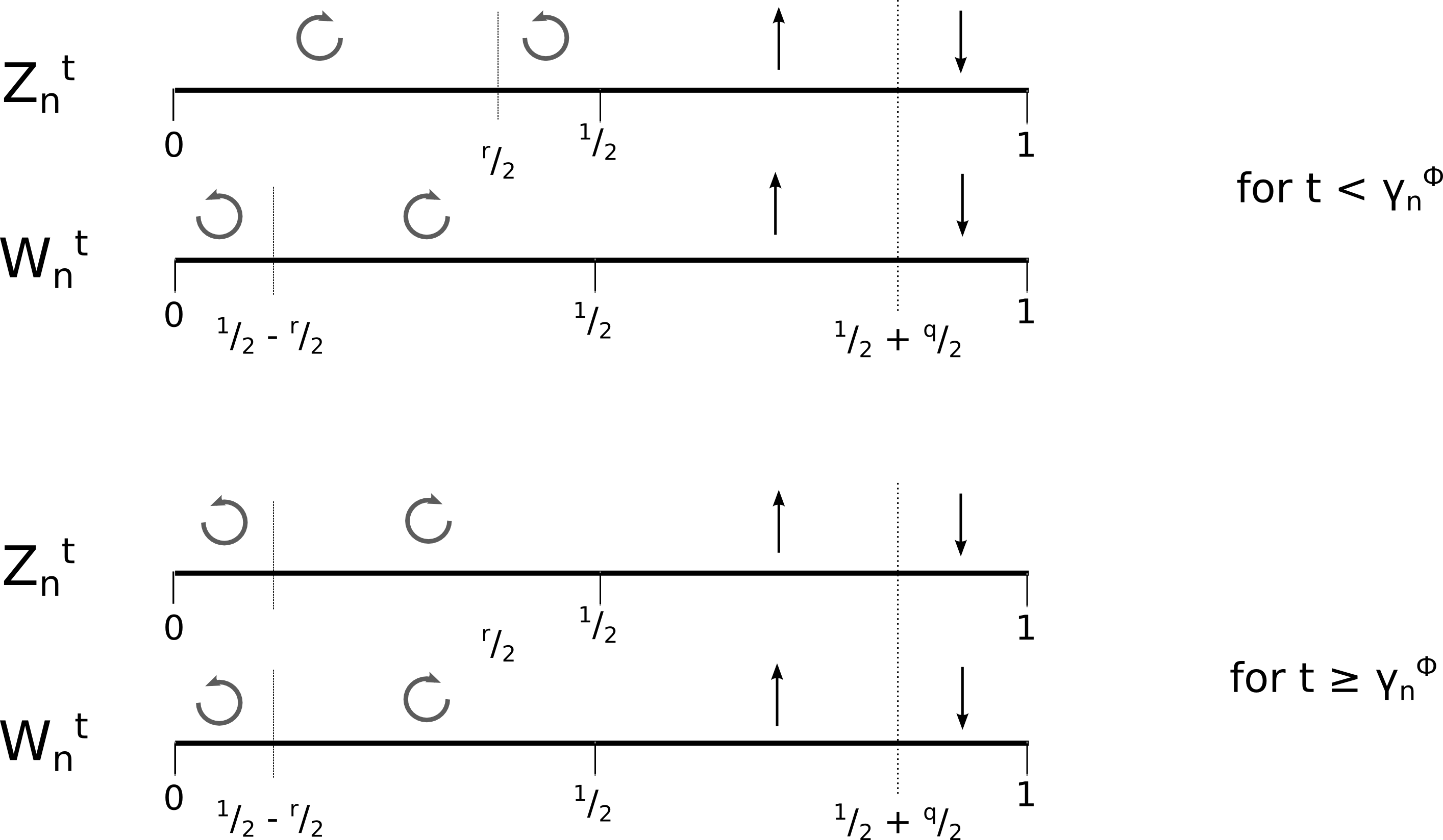
Figure 2: Coupling scheme, the same random update is used for both $Z_{n}^{t}$ and $W_{n}^{t}$. The two copies have the same probability to move to the upper or lower layer, except when one of the chains is on the topmost or bottommost layer. In the latter case the distance $H_{n}^{t}$ has probability $\frac{q}{2}$ to reduce by 1 while in the former it has probability $\frac{1-q}{2}$.

From the description of our coupling it should be clear that

$$\gamma_{n}=\max\{\gamma_{n}^{H},\gamma_{n}^{\Phi}\}\leq\gamma_{n}^{H}+\gamma_{n}^{\Phi}$$ (3.39)

Thus, using Markov’s inequality we get

$$\mathbb{P}\left(\gamma_{n}\geq\theta\delta_{n}\right) \leq\frac{\mathbb{E}\left[\gamma_{n}\right]}{\theta\delta_{n}}\leq\frac{\mathbb{E}\left[\gamma_{n}^{H}\right]+\mathbb{E}\left[\gamma_{n}^{\Phi}\right]}{\theta\delta_{n}}$$ (3.40)

Now, according to point 3 listed above and the transition probabilities of $W_{n}^{\sharp,t}=h(W_{n}^{t})$ we easily obtain

$$\mathbb{E}\left[\gamma_{n}^{H}\,\left|\,h(W_{n}^{0})=h^{\prime}\right.\right]=\beta^{-1}h^{\prime}$$ (3.41)

which yields to

$$\mathbb{E}\left[\gamma_{n}^{H}\right]=\beta^{-1}\mathbb{E}\left[h(W_{n}^{0})\right]=\beta^{-1}\sum_{x}x\,\pi_{n}^{\sharp}(x)\leq\beta^{-1}\frac{1-q}{2q-1}$$ (3.42)

According to point 4 listed above we get

$$\mathbb{E}\left[\gamma_{n}^{\Phi}\right]\propto m^{2}$$ (3.43)

Lines (3.42) and (3.43) clearly infer (3.37) and the proof is complete: the model exhibit cutoff at cutoff-time

$$a_{n}=\beta^{-1}l=\beta^{-1}n^{1-\omega}$$ (3.44)

and cutoff-window

$$b_{n}=O(m^{2}+\sqrt{l})=O\left(n^{2\omega}+n^{\frac{1-\omega}{2}}\right)$$ (3.45)

Remark 3.5.

The condition $\frac{b_{n}}{a_{n}}=o(1)$ is fulfilled only if $\omega<\frac{1}{3}$. Within this constraint we have cutoff and the cutoff-window shows the following behavior:

$$0<\omega\leq\frac{1}{5} \qquad b_{n}=O\left(n^{\frac{1-\omega}{2}}\right)$$

$$\frac{1}{5}\leq\omega<\frac{1}{3} \qquad b_{n}=O\left(n^{2\omega}\right)$$

and we see that the value $\omega=\frac{1}{5}$ gives the smallest cutoff-window order achievable.

Remark 3.6.

The case $\omega=0$ corresponds to an increase of the cylinder volume by extending its height while keeping fixed its base diameter, and it is almost identical to a biased random walk on a segment [6, §18.2.1]. In this sense the general case $\omega>0$ represents a non-reversible higher-dimensional extension of the biased random walk.

3.5 A partially-diffusive random walk

Fix $\varepsilon\in(0,\frac{1}{2})$ and consider the birth-and-death chain $X_{n}^{t}$ defined on the state space $\Omega_{n}=\{0,1,\ldots,n\}$ with initial position $X_{n}^{0}=n$ and transition rates

$$q_{i}=P_{i,i-1} =\begin{cases}\frac{i}{2n}&\quad\text{if }n^{\varepsilon}<i\leq n\\ \frac{1}{2}&\quad\text{if }1\leq i\leq n^{\varepsilon}\end{cases}$$ (3.46)

$$r_{i}=P_{i,i} =\begin{cases}1-p_{i}-q_{i}&\quad\text{if }n^{\varepsilon}\leq i\leq n\\ 0&\quad\text{if }0\leq i<n^{\varepsilon}\end{cases}$$ (3.47)

$$p_{i}=P_{i,i+1} =\begin{cases}\frac{i}{4n}&\quad\text{if }n^{\varepsilon}\leq i\leq n\\ \frac{1}{2}&\quad\text{if }0\leq i<n^{\varepsilon}\end{cases}$$ (3.48)

This chain is such that outside the interval $[0,n^{\varepsilon}]$ it behaves like a biased random walk while inside the interval it behaves like an unbiased one. It’s quite easy to show that this model does not satisfies the strong drift condition, which according to [3] is a sufficient condition to prove cutoff, see Remark 3.9 below. Using Corollary 1.3 it’s easy to show that this model actually exhibits cutoff.

The stationary distribution $\pi_{n}$ can be found by reversibility

$$\pi_{n}(i)=\begin{cases}c&\quad\text{for }0\leq i\leq n^{\varepsilon}\\ c\,\left(\frac{1}{2}\right)^{i-n^{\varepsilon}}&\quad\text{for }n^{\varepsilon}<i\leq n\\ \end{cases}$$ (3.49)

where the constant $c$ is $\frac{1}{n^{\varepsilon}+2}+O\left(\frac{1}{2^{n}}\right)$. In order to use Theorem 1.2 it is enough to take the following family of nested subsets

$$A_{n,\theta}=\{i\>:\>0\leq i\leq n^{\varepsilon}\theta^{n^{2\varepsilon-1}}\}$$ (3.50)

With this choice (1.17) holds and, to the leading order in $n$

$$\mathbb{E}\left[\zeta_{n}^{1}\right]=\frac{2(1-\varepsilon)}{\log 2}\>n\log n\qquad\quad\mathbb{E}\left[\zeta_{n}^{1}-\zeta_{n}^{\theta}\right]=\frac{2}{\log 2}n^{2\varepsilon}\log\theta\\$$ (3.51)

see Appendix B for the details of the calculations. Choosing $\Delta_{n}=n^{2\varepsilon}$ we verify (1.20) and (1.21), then by Remark 1.3 we know that all the hypotheses hold except possibly (1.18).

Now we consider a coupling $(Z_{n}^{t},W_{n}^{t})$, where $Z_{n}^{t}$ and $W_{n}^{t}$ are two copies of $X_{n}^{t}$ with initial positions $Z_{n}^{0}=n^{\varepsilon}$ and $W_{n}^{0}\sim\pi_{n}$ respectively; then, provided that the two chains have not yet collided, at each time we let the two copies evolve independently. Let $\gamma_{n}=\min\{t\geq 0\>:\>Z_{n}^{t}=W_{n}^{t}\}$ be the coalescence time and set $Z_{n}^{t}=W_{n}^{t}$ for any $t\geq\gamma_{n}$, then

$$\mathbb{P}\left(\gamma_{n}>t\,|\,Z_{n}^{0}=n^{\varepsilon}\right) =\mathbb{P}\left(\gamma_{n}>t\,|\,Z_{n}^{0}=n^{\varepsilon},W_{n}^{0}\leq n^{\varepsilon}\right)\mathbb{P}\left(W_{n}^{0}\leq n^{\varepsilon}\right)+$$

$$\quad\mathbb{P}\left(\gamma_{n}>t\,|\,Z_{n}^{0}=n^{\varepsilon},W_{n}^{0}>n^{\varepsilon}\right)\mathbb{P}\left(W_{n}^{0}>n^{\varepsilon}\right)$$ (3.52)

$$\leq\mathbb{P}\left(\gamma_{n}>t\,|\,Z_{n}^{0}=n^{\varepsilon},W_{n}^{0}\leq n^{\varepsilon}\right)+\frac{1}{n^{\varepsilon}}$$ (3.53)

Let $\tau_{n}^{0}=\min\{t\geq 0\>:\>Z_{n}^{t}=0\}$. Clearly,

$$\mathbb{P}\left(\gamma>t\,|\,Z_{n}^{0}=n^{\varepsilon},W_{n}^{0}\leq n^{\varepsilon}\right) \leq\mathbb{P}\left(\tau_{n}^{0}>t\,|\,Z_{n}^{t}=n^{\varepsilon}\right)$$ (3.54)

$$\leq\frac{\mathbb{E}\left[\tau_{n}^{0}\,|\,Z_{n}^{0}=n^{\varepsilon}\right]}{t}$$ (3.55)

where the last inequality comes from Markov’s inequality. Take $t=\theta n^{2\varepsilon}$, since $\mathbb{E}\left[\tau_{n}^{0}\,|\,Z_{n}^{0}=n^{\varepsilon}\right]=n^{2\varepsilon}+O(n^{\varepsilon})$, by Remark 2.2

$$\max_{z_{0}\in A_{n,1}}\mathbb{P}\left(\gamma_{n}>\theta n^{2\varepsilon}\,|\,Z_{n}^{0}=z_{0}\right)\leq\frac{2}{\theta}\text{ definitively as }n\to\infty$$ (1.26a)

The standard deviation of $\zeta_{n}^{1}$ is $O(n^{1-\frac{\varepsilon}{2}})$ (see Appendix B), therefore (1.18) holds and, with respect to the coupling defined above, (1.26) follows from (3.52)-(3.55) with $t=\theta\delta_{n}=2\theta\left(n^{2\varepsilon}+n^{1-\frac{\varepsilon}{2}}\right)$. Thus, by means of Theorem 1.2 and Corollary 1.3 we have that this model exhibits cutoff with cutoff-time

$$a_{n}=\mathbb{E}\left[\zeta_{n}^{1}\right]=\frac{2(1-\varepsilon)}{\log 2}\>n\log n$$ (3.56)

and cutoff window

$$b_{n}=\begin{cases}O(n^{1-\frac{\varepsilon}{2}})&\quad\text{if }0<\varepsilon\leq\frac{2}{5}\\ O(n^{2\varepsilon})&\quad\text{if }\frac{2}{5}<\varepsilon\leq\frac{1}{2}\end{cases}$$ (3.57)

Remark 3.7.

From 3.57 we see that the choice $\varepsilon=\frac{2}{5}$ gives the smallest cutoff-window order possible.

Remark 3.8.

This example shows how crucial is the choice of $\{A_{n,\theta}\}$. One could try in fact $A_{n,\theta}=\{i\>:\>0\leq i\leq\theta n^{\varepsilon}\}$, because that scaling, linear on $\theta$, worked well in the lazy Ehrenfest chain. This alternative definition would lead to an expected travelling time $\mathbb{E}\left[\zeta_{n}^{1}-\zeta_{n}^{\theta}\right]=n\log\theta$ and force $\Delta_{n}$ (and consequently $\delta_{n}$) to be of order $n$. Since $\theta n$ steps are clearly sufficient for the chain started in $n^{\varepsilon}$ to achieve equilibrium, we would obtain a non-optimal $O(n)$ cutoff-window.

Remark 3.9.

The reason why $X_{n}^{t}$ does not satisfies the strong drift condition is that it fails the first requirement of the definition, namely

$$K_{q}=\inf_{n\in\mathbb{N}}\inf_{0\leq i\leq n}q_{i}>0$$ (3.58)

Nevertheless, it is clear from the results included in [3] that the condition $K_{q}>0$ can actually be dropped if one replaces the second condition with

$$\frac{K^{2}_{n}}{K_{q}^{n}\,\mathbb{E}\left[T^{(n)}_{n\to 0}\right]}\TendsTo[n,\infty]0$$ (3.59)

where $K_{q}^{n}=\inf\limits_{0\leq i\leq n}q_{i}$ and

$$K_{n}=\sup_{1\leq i\leq n}q_{i}\,\mathbb{E}\left[T^{(n)}_{i\to i-1}\right]=\sup_{0\leq i\leq n}\frac{\pi_{n}([i,n])}{\pi_{n}(i)}$$ (3.60)

The expected value of $T^{(n)}_{n\to 0}$, the hitting time of zero starting from $n$, can be easily estimated as

$$\mathbb{E}\left[T^{(n)}_{n\to 0}\right]\leq O(n\log n+n^{2\varepsilon})\\$$ (3.61)

while $K_{n}$ can be bounded from below by $n^{\varepsilon}$. Then

$$\frac{K^{2}_{n}}{K_{q}^{n}\,\mathbb{E}\left[T^{(n)}_{n\to 0}\right]}\geq\frac{n^{2\varepsilon}}{\frac{n^{\varepsilon}}{2n}\left[O(n\log n+n^{2\varepsilon})\right]}\>\TendsTo[n,\infty]\infty$$ (3.62)

3.6 The mean-field Ising model Glauber dynamics

The cutoff for the mean-field Ising model evolving according to the Glauber dynamics has been recently proved in [2]. Here we give an alternative proof of the existence of the cutoff and we evaluate the cutoff-time and the cutoff-window in terms of an hitting process by means of our Corollary 1.3. The computations needed to achieve this goal in our framework are quite shortened. A generalization of this result to the non-symmetrical case, i.e. when a constant magnetic field is added, is likely to be treatable with little effort.

In the mean-field Ising model we have $n$ binary spins and a neighborhood structure given by a complete graph $K_{n}$. $\mathcal{X}_{n}=\{+1,-1\}^{n}$ is the set of all possible configurations. The energy of a configuration $\sigma=(\sigma_{1},\sigma_{2},\ldots,\sigma_{n})$ is then

$$H(\sigma)=-\frac{1}{n}\sum_{i<j}\sigma_{i}\,\sigma_{j}$$ (3.63)

The Glauber dynamics for this model is defined as follows:

• pick up a site $i\in\{1,2,\ldots,n\}$ uniformly at random

• update $\sigma_{i}$ to the values $+1$ or $-1$ respectively with probability

  $$p_{+} =\frac{e^{\beta\,S(i)}}{e^{\beta\,S(i)}+e^{-\beta\,S(i)}}$$ (3.64)

  $$p_{-} =\frac{e^{-\beta\,S(i)}}{e^{\beta\,S(i)}+e^{-\beta\,S(i)}}$$ (3.65)

  where $S(i)=\frac{1}{n}\sum_{j\not=i}\sigma_{j}$ is the so-called local field.

The parameter $\beta$ has the physical meaning of the inverse temperature of the system: the higher its value, the stronger the role of the energy over the entropy in the establishment of the equilibrium states. The limiting case of $\beta=0$ coincides with the lazy random walk on the hypercube seen in Section 3.3.1: all the spins are updated independently and they are equivalent from an energy-landscape point of view.

By reversibility it’s easy to show that the Markov chain defined above has a unique stationary measure

$$\rho_{n}(\sigma)=\frac{e^{-\beta\,H(\sigma)}}{Z_{n,\beta}}$$ (3.66)

where $Z_{n,\beta}=\sum_{\sigma^{\prime}\in\Omega_{n}}e^{-\beta\,H(\sigma^{\prime})}$ is the partition function.

Let us now define the magnetization of a configuration as

$$m(\sigma)=\frac{1}{2}\sum_{i}\sigma_{i}$$ (3.67)

Please note that this is not the standard definition of magnetization, since the one just defined in (3.67) takes values in $\Omega_{n}=\{-\frac{n}{2},-\frac{n}{2}+1,\ldots,\frac{n}{2}-1,\frac{n}{2}\}$ while in general $m\in[-1,1]$. We chose this definition because we want to reduce our system to a birth-and-death chain. We can rewrite the Hamiltonian (3.63) in terms of $m(\sigma)$ as follows:

$$m^{2}(\sigma) =\frac{1}{4}\left(\sum_{i}\sigma_{i}\right)\,\left(\sum_{j}\sigma_{j}\right)=\frac{n}{4}-\frac{n}{2}H(\sigma)$$ (3.68)

and then

$$H(m(\sigma))=-\frac{2m^{2}(\sigma)}{n}+\frac{1}{2}$$ (3.69)

The stationary distribution and the update probabilities take now the form

$$\rho_{n}(m(\sigma))=\frac{e^{\frac{2\beta}{n}m^{2}(\sigma)}}{Z^{\prime}_{n,\beta}}$$ (3.66a)

$$p_{+}=\frac{e^{\frac{2\beta}{n}(m(\sigma)-\sigma_{i})}}{e^{\frac{2\beta}{n}(m(\sigma)-\sigma_{i})}+e^{-\frac{2\beta}{n}(m(\sigma)-\sigma_{i})}}=\frac{1}{1+e^{-\frac{4\beta}{n}(m(\sigma)-\sigma_{i})}}$$ (3.64a)

$$p_{-}=\frac{e^{-\frac{2\beta}{n}(m(\sigma)-\sigma_{i})}}{e^{\frac{2\beta}{n}(m(\sigma)-\sigma_{i})}+e^{-\frac{2\beta}{n}(m(\sigma)-\sigma_{i})}}=\frac{1}{1+e^{\frac{4\beta}{n}(m(\sigma)-\sigma_{i})}}$$ (3.65a)

Let us now define the magnetization chain, that is a new birth-and-death chain $X_{n}^{t}$ with state space given $\Omega_{n}=\{-\frac{n}{2},-\frac{n}{2}+1,\ldots,\frac{n}{2}-1,\frac{n}{2}\}$ and transition rates

$$p_{k} =P_{k,k+1}=\frac{\frac{n}{2}-k}{n}\,\frac{1}{1+e^{-\frac{4\beta}{n}(k+1)}}$$ (3.70)

$$q_{k} =P_{k,k-1}=\frac{\frac{n}{2}+k}{n}\,\frac{1}{1+e^{\frac{4\beta}{n}(k-1)}}$$ (3.71)

$$r_{k} =P_{k,k}=\frac{1}{2}+\frac{k}{n}\tanh\left(\frac{4\beta}{n}(k+1)\right)$$ (3.72)

Using standard techniques it is possible to show that the magnetization chain is actually the projection of the Glauber chain according to the following equivalence relation

$$\sigma\sim\sigma^{\prime}\quad\Longleftrightarrow\quad m(\sigma)=m(\sigma^{\prime})$$ (3.73)

see for example [4, Thm. 5.1.4.1].

Consider the Glauber chain, started say with initial distribution $\lambda_{n}^{0}$ on $\mathcal{X}_{n}$ such that $\lambda_{n}^{0}(\sigma)=\lambda_{n}^{0}(\sigma^{\prime})$ whenever $\sigma\sim\sigma^{\prime}$. Along with this process take its projection, the magnetization chain, that has initial distribution $\mu_{n}^{0}$ and stationary measure $\pi_{n}$ equal to

$$\mu_{n}^{0}(k) =\sum_{\sigma\>:\>m(\sigma)=k}\lambda_{n}^{0}(\sigma)$$ (3.74)

$$\pi_{n}(k) =\sum_{\sigma\>:\>m(\sigma)=k}\rho_{n}(\sigma)=\frac{e^{\frac{2\beta k^{2}}{n}}}{Z_{n,\beta}}{n\choose\frac{n}{2}+k}$$ (3.75)

It is not difficult whatsoever to prove that $\lambda_{n}^{0}(\sigma)=\lambda_{n}^{0}(\sigma^{\prime})$ for $\sigma\sim\sigma^{\prime}$ leads to $\lambda_{n}^{t}(\sigma)=\lambda_{n}^{t}(\sigma^{\prime})$ for any $t\geq 0$, which in turn infers that

$$d_{\text{\tiny TV}}\left(\lambda_{n}^{t},\rho_{n}\right)=d_{\text{\tiny TV}}\left(\mu_{n}^{t},\pi_{n}\right)\quad\forall\,t\geq 0$$ (3.76)

In other words, the Glauber chain exhibit cutoff if and only if the magnetization chain does.

3.6.1 Analysis of $\pi_{n}(k)$

Fix $\theta\geq 1$ and define

$$A_{n,\theta}=\left\{k\in\Omega_{n}\>:\>-\theta\sqrt{\frac{n}{1-\beta}}\leq k\leq\theta\sqrt{\frac{n}{1-\beta}}\right\}$$ (3.77)

For $k\in A_{n,\theta}$ we can estimate $\pi_{n}(k)$ by means of Stirling’s formula:

$${n\choose\frac{n}{2}+k} =\frac{2^{n+\frac{1}{2}}}{\sqrt{\pi n\left(1-\frac{4k^{2}}{n^{2}}\right)}}\frac{(1+O\left(n^{-1}\right))}{\left(1+\frac{2k}{n}\right)^{\frac{n}{2}\left(1+\frac{2k}{n}\right)}\left(1-\frac{2k}{n}\right)^{\frac{n}{2}\left(1-\frac{2k}{n}\right)}}$$ (3.78)

Next we pass to the log and use its analytic expansion to get

$$\log\frac{1}{\left(1+\frac{2k}{n}\right)^{\frac{n}{2}\left(1+\frac{2k}{n}\right)}\left(1-\frac{2k}{n}\right)^{\frac{n}{2}\left(1-\frac{2k}{n}\right)}}=-\frac{n}{2}\left[\sum_{i\geq 1}\left(\frac{2k}{n}\right)^{2i}\frac{1}{2i^{2}-i}\right]$$ (3.79)

Therefore for $k\in A_{n,\theta}$ we have

$$\pi_{n}(k) =\frac{2^{n+\frac{1}{2}}}{Z_{n,\beta}}\sqrt{\frac{1}{\pi n}}e^{-\frac{2(1-\beta)}{n}k^{2}}(1+O\left(n^{-1}\right))$$ (3.80)

that is $\pi_{n}(k)$ is very close to a Gaussian distribution $\mathcal{N}\left(0,\frac{1}{2}\sqrt{\frac{n}{1-\beta}}\right)$ for $k\in A_{n,\theta}$. This means that (1.17) holds, because there exists a positive constant $c_{\beta}$ such that, for $n$ sufficiently large

$$\pi_{n}\left(A_{n,\theta}^{\complement}\right)<\frac{c_{\beta}}{\theta^{2}}$$ (3.81)

Remark 3.10.

Note that in this model the Gaussian structure of $\pi_{n}$ is given by both energy and entropy contribution, merging in the expression of the free-energy, which can be recognized as the exponent of $e^{-\frac{2(1-\beta)}{n}k^{2}}$ divided by $\beta$. Hence in this case we will say that the cutoff is free-energy driven.

3.6.2 Proof of cutoff

Now suppose the Glauber chain is started at time $0$ with magnetization $\frac{n}{2}$, that is $\lambda_{n}^{0}=\delta_{\sigma,1}$ and $\mu_{n}^{0}=\delta_{i,\frac{n}{2}}$; this choice gives equal probability to equivalent configurations, then (3.76) holds. As usual define $\zeta_{n}^{\theta}$ as the hitting time of $A_{n,\theta}$ and $\zeta_{n}^{1}$ as the hitting time of $A_{n,1}$. Lengthy but straightforward calculations (deferred to Appendix A) show that, to the leading order in $n$

$$\mathbb{E}\left[\zeta_{n}^{1}\right]=\frac{1}{2(1-\beta)}n\log n$$ (3.82)

$$\mathbb{E}\left[\zeta_{n}^{1}-\zeta_{n}^{\theta}\right]=(1+\log\theta)\,O(n)$$ (3.83)

and that $\text{Var}[\zeta_{n}^{1}]$ grows at most as $O(n^{2})$; Therefore hypotheses (1.18)-(2.38) are satisfied. Moreover, choose $\Delta_{n}=O(n)$, $\delta_{n}$ is now of order $n$ and both (1.20) and (1.21) are fulfilled, so that Theorem 1.2 gives us (1.22). Then we are left to prove that with $\delta_{n}=O(n)$ Corollary 1.3 holds.

Remark 3.11.

Since for $\beta=0$ the magnetization chain reduces to the Ehrenfest chain, the following estimates hold as well for the Ehrenfest Urn model presented in Section 3.3.

To prove Corollary 1.3 consider the following coupling, $(Z_{n}^{t},W_{n}^{t},Z_{n}^{+,t},Z_{n}^{-,t})$ where each component is a copy of the magnetization chain and

$$\begin{array}[]{lcl}Z_{n}^{0}=z_{0}\equiv\frac{1}{2}\sqrt{\frac{n}{1-\beta}}&&Z_{n}^{+,t}=z_{0}^{+}\equiv z_{0}\theta^{\frac{1}{3}}\\ W_{n}^{0}\sim\pi_{n}&&Z_{n}^{-,t}=z_{0}^{-}\equiv-z_{0}\theta^{\frac{1}{3}}\end{array}$$ (3.84)

for a given fixed $\theta>1$. Let any of the four chains move according with the same transition probabilities and using the same i.i.d. random update $u\sim U(0,1)$. To illustrate the transition probabilities let us consider for instance the chain $Z_{n}^{t}$ and suppose that at time $t$ we have $Z_{n}^{t}=k$, then

$$\text{if }k\geq 0 \qquad\begin{cases}Z_{n}^{t+1}=Z_{n}^{t}+1&\text{if }0\leq u<p_{k}\\ Z_{n}^{t+1}=Z_{n}^{t}&\text{if }p_{k}\leq u\leq 1-q_{k}\\ Z_{n}^{t+1}=Z_{n}^{t}-1&\text{if }1-q_{k}<u\leq 1\end{cases}$$

$$\text{if }k<0 \qquad\begin{cases}Z_{n}^{t+1}=Z_{n}^{t}-1&\text{if }0\leq u<q_{k}\\ Z_{n}^{t+1}=Z_{n}^{t}&\text{if }q_{k}\leq u\leq 1-p_{k}\\ Z_{n}^{t+1}=Z_{n}^{t}+1&\text{if }1-p_{k}<u\leq 1\end{cases}$$

The restriction of the coupling defined above to its first two components, $Z_{n}^{t}$ and $Y_{n}^{t}$, is the coupling we are going to consider for Corollary 1.3. Thus we define $\gamma_{n}=\min\{t\geq 0\,:\,Z_{n}^{t}=W_{n}^{t}\}$ and recall Remark 2.2.

By a careful analysis of (3.70)-(3.72) (noticing, in particular, that $r_{k}\geq\frac{1}{2}$ and $p_{k}=q_{-k}$) such a scheme ensures that any two components of the coupling mantain their relative partial order undergoing a single-step transition, and indeed it is impossible that two chains at distance $1$ will undergo a one step transition that would change their relative order.

Hence the evolution scheme described above has the following sandwiching properties

1. $Z_{n}^{+,t}=-Z_{n}^{-,t}$

2. $Z_{n}^{-,t}\leq Z_{n}^{t}\leq Z_{n}^{+,t}$

3. $Z_{n}^{-,t}\leq W_{n}^{t}\leq Z_{n}^{+,t}$ provided that $W_{n}^{0}\in A_{n,\theta^{\frac{1}{3}}}$

Using (3.81) we have

$$\mathbb{P}\left(\gamma_{n}>t\,|\,Z_{n}^{0}=z_{0}\right) =\mathbb{P}\left(\gamma_{n}>t\,\left|\,Z_{n}^{0}=z_{0},W_{n}^{0}\in A_{n,\theta^{\frac{1}{3}}}\right.\right)\mathbb{P}\left(W_{n}^{0}\in A_{n,\theta^{\frac{1}{3}}}\right)+$$

$$\mathbb{P}\left(\gamma_{n}>t\,\left|\,Z_{n}^{0}=z_{0},W_{n}^{0}\not\in A_{n,\theta^{\frac{1}{3}}}\right.\right)\mathbb{P}\left(W_{n}^{0}\not\in A_{n,\theta^{\frac{1}{3}}}\right)$$ (3.85)

$$\leq\mathbb{P}\left(\gamma_{n}>t\,\left|\,Z_{n}^{0}=z_{0},W_{n}^{0}\in A_{n,\theta^{\frac{1}{3}}}\right.\right)+\frac{c_{\beta}}{\theta^{\frac{2}{3}}}$$ (3.86)

Therefore by means of the sandwiching properties stated above

$$\mathbb{P}\left(\gamma_{n}>t\,\left|\,Z_{n}^{0}=z_{0},W_{n}^{0}\in A_{n,\theta^{\frac{1}{3}}}\right.\right)\leq\mathbb{P}\left(\tau^{0}_{n}>t\,|\,Z_{n}^{+,0}=z_{0}^{+}\right)$$ (3.87)

where $\tau_{n}^{0}=\min\{t\geq 0\>:\>Z_{n}^{+,t}=Z_{n}^{-,t}=0\}$. Note that $Z_{n}^{+,t}$ has a drift towards 0 as well as any copy of the magnetization chain. Accordingly, it can be coupled with a lazy uniform random walk $R_{n}^{t}$ such that

$$R_{n}^{0}=z_{0}^{+}$$ (3.88)

$$\mathbb{P}\left(\tau_{n}^{0}>t\,|\,Z_{n}^{+,0}=z_{0}^{+}\right)\leq\mathbb{P}\left(\tilde{\tau}_{n}^{0}>t\,|\,R_{n}^{0}=z_{0}^{+}\right)$$ (3.89)

where $\tilde{\tau}_{n}^{0}=\min\{t\geq 0\>:\>R_{n}^{t}=0\}.$ Now we can use the following estimate, which is a classical result for random walks

$$\mathbb{P}\left(\tilde{\tau}_{n}^{0}>t\,|\,R_{n}^{0}=z_{0}^{+}\right)\leq\frac{c\,z_{0}^{+}}{\sqrt{t}}$$ (3.90)

and we have found that Corollary 1.3 holds with $\delta_{n}=n$.

Appendix A Mean value and variance of $\zeta_{n}^{1}$ for the mean-field Ising model

In this appendix we present in full details the estimates for $\mathbb{E}\left[\zeta_{n}^{1}\right]$ and $\text{Var}[\zeta_{n}^{1}]$ we have used to apply Corollary 1.3 to the magnetization chain in Section 3.6. Since for $\beta=0$ the magnetization chain reduces to the Ehrenfest chain, the following estimates hold as well for the Ehrenfest Urn model presented in Section 3.3.

Standard formulas (see e.g. [3]) give

$$\mathbb{E}\left[\zeta_{n}^{1}\right] =\sum_{k=\frac{1}{2}\sqrt{\frac{n}{1-\beta}}+1}^{\frac{n}{2}}\mathbb{E}\left[\zeta_{k\to k-1}\right]=\sum_{k=\frac{1}{2}\sqrt{\frac{n}{1-\beta}}+1}^{\frac{n}{2}}\frac{1}{q_{k}}\sum_{j=k}^{\frac{n}{2}}\frac{\pi_{n}(j)}{\pi_{n}(k)}$$ (A.1)

$$\text{Var}[\zeta_{n}^{1}] =\sum_{k=\frac{1}{2}\sqrt{\frac{n}{1-\beta}}+1}^{\frac{n}{2}}\text{Var}[\zeta_{k\to k-1}]$$

$$=\sum_{k=\frac{1}{2}\sqrt{\frac{n}{1-\beta}}+1}^{\frac{n}{2}}\frac{1}{q_{k}}\sum_{j=k}^{\frac{n}{2}}\left(2\mathbb{E}\left[\zeta_{j\to k-1}\right]-\mathbb{E}\left[\zeta_{k\to k-1}\right]\right)\frac{\pi_{n}(j)}{\pi_{n}(k)}-\mathbb{E}\left[\zeta_{n}^{1}\right]$$ (A.2)

where $\zeta_{k\to k-1}$ is the first time the chain visits $k-1$ after visiting $k$ and

$$q_{k}=\frac{n}{\frac{n}{2}+k}\left(1+e^{\frac{4\beta}{n}(k-1)}\right)$$ (A.3)

$$\frac{\pi_{n}(j)}{\pi_{n}(k)}=\frac{{n\choose\frac{n}{2}+j}}{{n\choose\frac{n}{2}+k}}e^{\frac{2\beta}{n}(j^{2}-k^{2})}$$ (A.4)

Let us begin rewriting the ratio of the two binomial coefficients as

$$\frac{{n\choose\frac{n}{2}+j}}{{n\choose\frac{n}{2}+k}} =\prod_{i=0}^{j-k-1}\frac{\frac{n}{2}-k-i}{\frac{n}{2}+k+i+1}$$

$$=\left(\frac{\frac{n}{2}-k}{\frac{n}{2}+k+1}\right)^{j-k}\;\prod_{i=0}^{j-k-1}\left(1-\frac{i}{\frac{n}{2}-k}\right)\left(\frac{1}{1+\frac{i}{\frac{n}{2}+k+1}}\right)$$ (A.5)

Next, note that for any of the values of triple $(i,j,k)$ involved in the calculations

$$0\leq\frac{i}{\frac{n}{2}+k+1}\leq\frac{i}{\frac{n}{2}-k}\leq 1$$ (A.6)

So we find handy the following two easy lemmas.

Lemma A.1.

For $x\in[0,1]$

$$(1-x)\frac{1}{1+x}\leq e^{-2x}$$ (A.7)

Lemma A.2.

For $0\leq y\leq x\leq 1$

$$(1-x)\frac{1}{1+y}\leq e^{-x-y}$$ (A.8)

In virtue of Lemma A.2 we can bound line (A.5) as follows:

$$\frac{{n\choose\frac{n}{2}+j}}{{n\choose\frac{n}{2}+k}} \leq\left(\frac{\frac{n}{2}-k}{\frac{n}{2}+k}\right)^{j-k}\,e^{-\sum_{i=0}^{j-k-1}\left[\frac{i}{\frac{n}{2}-k}+\frac{i}{\frac{n}{2}+k+1}\right]}$$ (A.9)

$$=\left(\frac{\frac{n}{2}-k}{\frac{n}{2}+k}\right)^{j-k}\,e^{\frac{-2(j-k)^{2}+2(j-k)}{n\left(1-\frac{4k^{2}}{n^{2}}+\frac{2}{n}-\frac{4k}{n^{2}}\right)}}e^{\frac{-2(j-k)^{2}+2(j-k)}{n^{2}\left(1-\frac{4k^{2}}{n^{2}}+\frac{2}{n}-\frac{4k}{n^{2}}\right)}}$$ (A.10)

$$\leq\left(\frac{\frac{n}{2}-k}{\frac{n}{2}+k}\right)^{j-k}\,e^{\frac{-2(j-k)^{2}+2(j-k)}{n\left(1-\frac{4k^{2}}{n^{2}}+\frac{2}{n}-\frac{4k}{n^{2}}\right)}}$$ (A.11)

Thus, for $\frac{1}{2}\sqrt{\frac{n}{1-\beta}}\leq k\leq\frac{n}{2}-\log n$,

$$\sum_{j=k}^{\frac{n}{2}}\frac{{n\choose\frac{n}{2}+j}}{{n\choose\frac{n}{2}+k}}e^{\frac{2\beta}{n}(j^{2}-k^{2})} \leq\sum_{j=k}^{\frac{n}{2}}\left(\frac{\frac{n}{2}-k}{\frac{n}{2}+k}\right)^{j-k}\,e^{\frac{-2(j-k)^{2}+2(j-k)}{n\left(1-\frac{4k^{2}}{n^{2}}+\frac{2}{n}-\frac{4k}{n^{2}}\right)}}e^{\frac{2\beta}{n}(j^{2}-k^{2})}$$ (A.12)

$$\leq\sum_{l=0}^{\frac{n}{2}-k}\left(\frac{\frac{n}{2}-k}{\frac{n}{2}+k}\,e^{\frac{4\beta k}{n}}\right)^{l}\,e^{\frac{-2(1-\beta)l^{2}+2l}{n\left(1-\frac{4k^{2}}{n^{2}}+\frac{2}{n}-\frac{4k}{n^{2}}\right)}}$$ (A.13)

$$\leq\sum_{l=0}^{\infty}\left(\frac{\frac{n}{2}-k}{\frac{n}{2}+k}\,e^{\frac{4\beta k}{n}}\right)^{l}\,\left(1+O\left(\log^{-1}n\right)\right)$$ (A.14)

$$=\frac{\left(\frac{n}{2}+k\right)\left(1+O\left(\log^{-1}n\right)\right)}{\frac{n}{2}\left(1-e^{\frac{4\beta k}{n}}\right)+k\left(1+e^{\frac{4\beta k}{n}}\right)}$$ (A.15)

$$\leq\frac{\frac{n}{2}+k}{2(1-\beta)k}\,\left(1+O\left(\log^{-1}n\right)\right)$$ (A.16)

Therefore we obtain the following upper bounds:

$$\mathbb{E}\left[\zeta_{n}^{1}\right] \leq\frac{n}{2(1-\beta)}\left[\sum_{k=\frac{1}{2}\sqrt{\frac{n}{1-\beta}}+1}^{\frac{n}{2}-\log n}\frac{1+e^{\frac{4\beta k}{n}}}{k}\right]\,\left(1+O\left(\log^{-1}n\right)\right)$$

$$\qquad+c_{1}\,\sum_{k=\frac{n}{2}-\log n}^{\frac{n}{2}}\frac{n}{\frac{n}{2}+k}\left(1+e^{\frac{4\beta}{n}(k-1)}\right)\sum_{l=0}^{\frac{n}{2}-k}\left(c_{2}\frac{\log n}{n}\right)^{l}$$ (A.17)

$$=\frac{1}{2(1-\beta)}n\log n+O(n)$$ (A.18)

and

$$\mathbb{E}\left[\zeta_{n}^{1}-\zeta_{n}^{\theta}\right] \leq\frac{n}{2(1-\beta)}\left[\sum_{k=\frac{1}{2}\sqrt{\frac{n}{1-\beta}}+1}^{\frac{\theta}{2}\sqrt{\frac{n}{1-\beta}}}\frac{1+e^{\frac{4\beta k}{n}}}{k}\right]+O(n)$$ (A.19)

$$=(1+\log\theta)O(n)$$ (A.20)

From previous computations, noticing that

$$e^{\frac{-2(1-\beta)l^{2}+2l}{n\left(1-\frac{4k^{2}}{n^{2}}+\frac{2}{n}-\frac{4k}{n^{2}}\right)}}\leq\sqrt{e}$$ (A.21)

we have that

$$\mathbb{E}\left[\zeta_{k\to k-1}\right]\leq\sqrt{e}\>\frac{1+e^{\frac{4\beta k}{n}}}{2(1-\beta)}\frac{n}{k}$$ (A.22)

and then by summation

$$\mathbb{E}\left[\zeta_{k+l\to k-1}\right]\leq\frac{\sqrt{e}}{2(1-\beta}n\log\left(1+\frac{l}{k}\right)+O(n)$$ (A.23)

From (A.2), using (A.11) and (A.22)-(A.23), we can easily bound the variance of $\zeta_{k\to k-1}$ as follows:

$$\text{Var}[\zeta_{k\to k-1}] \leq\frac{n}{\frac{n}{2}+k}\left(1+e^{\frac{4\beta}{n}(k-1)}\right)\sum_{j=k}^{\frac{n}{2}}\mathbb{E}\left[\zeta_{j\to k-1}\right]\frac{{n\choose\frac{n}{2}+j}}{{n\choose\frac{n}{2}+k}}e^{\frac{2\beta}{n}(j^{2}-k^{2})}$$ (A.24)

$$\leq\frac{c_{\beta}\,n^{2}}{\frac{n}{2}+k}\sum_{l=0}^{\frac{n}{2}-k}\log\left(1+\frac{l}{k}\right)\left(\frac{\frac{n}{2}-k}{\frac{n}{2}+k}\,e^{\frac{4\beta k}{n}}\right)^{l}$$ (A.25)

$$\leq\frac{c_{\beta}\,n^{2}}{\frac{n}{2}+k}\sum_{l=0}^{\frac{n}{2}-k}\frac{l}{k}\left(\frac{\frac{n}{2}-k}{\frac{n}{2}+k}\,e^{\frac{4\beta k}{n}}\right)^{l}$$ (A.26)

$$\leq\frac{c_{\beta}\,n^{2}}{\frac{n}{2}+k}\,\frac{1}{k}\,\sum_{l=0}^{\infty}l\left(\frac{\frac{n}{2}-k}{\frac{n}{2}+k}\,e^{\frac{4\beta k}{n}}\right)^{l}$$ (A.27)

$$\leq\frac{c_{\beta}\,n^{2}}{\left(\frac{n}{2}+k\right)^{2}}\,\frac{1}{k}\,\left({\frac{n}{2}-k}\right)\,\left(\frac{\frac{n}{2}+k}{2(1-\beta)k}\right)^{2}$$ (A.28)

$$\leq c_{\beta}\frac{n^{3}}{k^{3}}$$ (A.29)

Therefore $\text{Var}[\zeta_{n}^{1}]=\sum_{k=\frac{1}{2}\sqrt{\frac{n}{1-\beta}}+1}^{\frac{n}{2}}\text{Var}[\zeta_{k\to k-1}]$ grows at most as $O(n^{2})$.

Eventually, let us bound from below the expectation $\mathbb{E}\left[\zeta_{n}^{1}\right]$. From (A.1) and (A.5) we have

$$\mathbb{E}\left[\zeta_{n}^{1}\right]\geq\sum_{\frac{1}{2}\log n\sqrt{\frac{n}{1-\beta}}}^{\frac{n}{\log n}}\frac{n}{\frac{n}{2}+k}\left(1+e^{\frac{4\beta k}{n}(k-1)}\right)\sum_{j=k}^{k+\frac{\sqrt{n}}{\log\log n}}\Bigg{[}\left(\frac{\frac{n}{2}-k}{\frac{n}{2}+k}\right)^{j-k}$$

$$\prod_{i=0}^{j-k-1}\left(1-\frac{i}{\frac{n}{2}-k}\right)\left(\frac{1}{1+\frac{i}{\frac{n}{2}+k+1}}\right)e^{\frac{2\beta}{n}(j^{2}-k^{2})}\Bigg{]}$$ (A.30)

Then we have

$$\sum_{j=k}^{k+\frac{\sqrt{n}}{\log\log n}}\left(\frac{\frac{n}{2}-k}{\frac{n}{2}+k}\right)^{j-k}\prod_{i=0}^{j-k-1}\left(1-\frac{i}{\frac{n}{2}-k}\right)\left(\frac{1}{1+\frac{i}{\frac{n}{2}+k+1}}\right)e^{\frac{2\beta}{n}(j^{2}-k^{2})}$$

$$\geq\sum_{j=k}^{k+\frac{\sqrt{n}}{\log\log n}}\left(\frac{\frac{n}{2}-k}{\frac{n}{2}+k}\right)^{j-k}\left(\prod_{i=0}^{j-k-1}\left(1-\frac{i}{\frac{n}{2}-k}\right)e^{-\frac{i}{\frac{n}{2}+k+1}}\right)e^{\frac{2\beta}{n}(j^{2}-k^{2})}$$ (A.31)

$$\geq\sum_{j=k}^{k+\frac{\sqrt{n}}{\log\log n}}\left[\left(\frac{\frac{n}{2}-k}{\frac{n}{2}+k}\right)^{j-k}\left(\prod_{i=0}^{j-k-1}e^{-\frac{i}{\frac{n}{2}-k}-\frac{i}{\frac{n}{2}+k+1}}\right)e^{\frac{2\beta}{n}(j^{2}-k^{2})}+\varepsilon_{1}\right]$$ (A.32)

where $\varepsilon_{1}$ tends to $0$ exponentially fast in $n$.

Remark A.1.

The error $\varepsilon_{1}$ gives a negligible contribution to $\mathbb{E}\left[\zeta_{n}^{1}\right]$ being exponentially small, for this reason we will henceforth drop it.

The right-hand in (A.32) can be rewritten as follows

$$\sum_{j=k}^{k+\frac{\sqrt{n}}{\log\log n}}\left(\frac{\frac{n}{2}-k}{\frac{n}{2}+k}\right)^{j-k}e^{\frac{-2(j-k)^{2}+2(j-k)}{n\left(1-\frac{4k^{2}}{n^{2}}+\frac{2}{n}-\frac{4k}{n^{2}}\right)}+\frac{-2(j-k)^{2}+2(j-k)}{n^{2}\left(1-\frac{4k^{2}}{n^{2}}+\frac{2}{n}-\frac{4k}{n^{2}}\right)}+\frac{2\beta}{n}(j^{2}-k^{2})}$$ (A.33)

$$=\sum_{l=0}^{\frac{\sqrt{n}}{\log\log n}}\left(\frac{\frac{n}{2}-k}{\frac{n}{2}+k}e^{\frac{4\beta k}{n}}\right)^{l}e^{\frac{-2l^{2}+2l}{n\left(1-\frac{4k^{2}}{n^{2}}+\frac{2}{n}-\frac{4k}{n^{2}}\right)}+\frac{-2l^{2}+2l}{n^{2}\left(1-\frac{4k^{2}}{n^{2}}+\frac{2}{n}-\frac{4k}{n^{2}}\right)}+\frac{2\beta}{n}l^{2}}$$ (A.34)

$$=\sum_{l=0}^{\frac{\sqrt{n}}{\log\log n}}\left(\frac{\frac{n}{2}-k}{\frac{n}{2}+k}e^{\frac{4\beta k}{n}}\right)^{l}e^{\frac{-2l^{2}+2l}{n\left(1-\frac{4k^{2}}{n^{2}}+\frac{2}{n}-\frac{4k}{n^{2}}\right)}+\frac{2\beta}{n}l^{2}}(1+\varepsilon_{2})$$ (A.35)

with $\varepsilon_{2}=o\left(n^{-1}\right)$. Now set $\varphi=-\frac{4k^{2}}{n^{2}}+\frac{2}{n}-\frac{4k}{n^{2}}$, then (A.35) can be rewritten as follows

$$\sum_{l=0}^{\frac{\sqrt{n}}{\log\log n}}\left(\frac{\frac{n}{2}-k}{\frac{n}{2}+k}e^{\frac{4\beta k}{n}}\right)^{l}e^{\frac{-2(1-\beta(1+\varphi))l^{2}}{n(1+\varphi)}+\frac{2l}{n(1+\varphi)}}(1+\varepsilon_{2})$$ (A.36)

$$=\sum_{l=0}^{\frac{\sqrt{n}}{\log\log n}}\left(\frac{\frac{n}{2}-k}{\frac{n}{2}+k}e^{\frac{4\beta k}{n}}\right)^{l}(1-\varepsilon)(1+\varepsilon_{3})(1+\varepsilon_{2})$$ (A.37)

$$=\sum_{l=0}^{\frac{\sqrt{n}}{\log\log n}}\left(\frac{\frac{n}{2}-k}{\frac{n}{2}+k}e^{\frac{4\beta k}{n}}\right)^{l}(1-\varepsilon)$$ (A.38)

where $\varepsilon=O\left(\log^{-2}(\log n)\right)$ and $\varepsilon_{3}=O\left(n^{-\frac{1}{2}}\log\log n\right)$.

Therefore

$$\mathbb{E}\left[\zeta_{n}^{1}\right]\geq(1-\varepsilon)\sum_{\frac{1}{2}\log n\sqrt{\frac{n}{1-\beta}}}^{\frac{n}{\log n}}\frac{n}{\frac{n}{2}+k}\left(1+e^{\frac{4\beta k}{n}(k-1)}\right)\sum_{l=0}^{\frac{\sqrt{n}}{\log\log n}}\left(\frac{\frac{n}{2}-k}{\frac{n}{2}+k}e^{\frac{4\beta k}{n}}\right)^{l}$$

$$=\mathbb{E}\left[\zeta_{n}^{1}\right]\geq(1-\varepsilon)\sum_{\frac{1}{2}\log n\sqrt{\frac{n}{1-\beta}}}^{\frac{n}{\log n}}\Bigg{\{}\frac{n}{\frac{n}{2}+k}\left(1+e^{\frac{4\beta k}{n}(k-1)}\right)$$

$$\qquad\frac{(\frac{n}{2}+k+1)}{\frac{n}{2}(1-e^{\frac{4\beta k}{n}})+k(1+e^{\frac{4\beta k}{n}})+1}\left[1-\left(\frac{\frac{n}{2}-k}{\frac{n}{2}+k+1}e^{\frac{4\beta k}{n}}\right)^{1+\frac{\sqrt{n}}{\log\log n}}\right]\Bigg{\}}$$

$$\geq(1-\gamma)(1-\varepsilon)\sum_{\frac{1}{2}\log n\sqrt{\frac{n}{1-\beta}}}^{\frac{n}{\log n}}\frac{n}{\frac{n}{2}+k}\left(2+O\left(\log^{-1}n\right)\right)\,\Gamma$$ (A.39)

where

$$\gamma=\left[\frac{1-\frac{\log n}{\sqrt{n(1-\beta)}}}{1+\frac{\log n}{\sqrt{n(1-\beta)}}}\left(1+2\beta\frac{\log n}{\sqrt{n(1-\beta)}}+O\left(\frac{\log^{2}n}{n}\right)\right)\right]^{1+\frac{\sqrt{n}}{\log\log n}}$$ (A.40)

and

$$\Gamma=\frac{\frac{n}{2}+k}{\frac{n}{2}(\frac{-4\beta k}{n}+O\left(\log^{-2}n\right))+k(2+\frac{4\beta k}{n}+O\left(\log^{-2}n\right))+2}$$ (A.41)

Now, $\gamma$ can be rewritten as

$$\gamma=\left[1-\frac{2(1-\beta)\log n}{\sqrt{n(1-\beta)}}+O\left(\frac{\log^{2}n}{n}\right)\right]^{1+\frac{\sqrt{n}}{\log\log n}}$$ (A.42)

Therefore $\gamma$ tends asintotically to $0$.

The right-hand in (A.39) now becomes

$$(1-\gamma)(1-\varepsilon)\sum_{\frac{1}{2}\log n\sqrt{\frac{n}{1-\beta}}}^{\frac{n}{\log n}}\frac{2n\left(1+O\left(\log^{-1}n\right)\right)}{2k(1-\beta)+2+O\left(\log^{-1}n\right)}$$ (A.43)

from which we see that, to the leading order in $n$

$$\mathbb{E}\left[\zeta_{n}^{1}\right]\geq\frac{1}{2(1-\beta)}n\log n$$ (A.44)

Appendix B Mean value and variance of $\zeta_{n}^{1}$ for the partially diffusive random walk

Standard formulas (see e.g. [3]) give

$$\mathbb{E}\left[\zeta_{n}^{1}\right] =\sum_{k=n^{\varepsilon}+1}^{n}\mathbb{E}\left[\zeta_{k\to k-1}\right]=\sum_{k=n^{\varepsilon}+1}^{n}\frac{2n}{k}\sum_{m=k}^{n}\frac{\pi_{n}(m)}{\pi_{n}(k)}$$ (B.1)

where $\zeta_{k\to k-1}$ is the first time the chain visits $k-1$ after visiting $k$. By means of (3.46)-(3.48) and reversibility,

$$\phi(k) =\sum_{m=k}^{n}\frac{\pi_{n}(m)}{\pi_{n}(k)}$$ (B.2)

$$=\sum_{m=k}^{n}\frac{k}{m}2^{k-m}$$ (B.3)

$$\simeq k2^{k}\int_{-k\log 2}^{-n\log 2}\frac{e^{t}}{t}\,dt$$ (B.4)

Using the properties of the exponential integral we get

$$\phi(k)=\frac{1}{\log 2}-\frac{k}{n\log 2}2^{(k-n)}+O\left(\frac{1}{k}\right)$$ (B.5)

and therefore

$$\mathbb{E}\left[\zeta_{n}^{1}\right]=\frac{2(1-\varepsilon)}{\log 2}n\log n+O\left(n^{1-\varepsilon}\right)$$ (B.6)

Similarly, for $n$ sufficiently large we have that

$$\mathbb{E}\left[\zeta_{n}^{1}-\zeta_{n}^{\theta}\right]=\sum_{k=n^{\varepsilon}+1}^{n^{\varepsilon}\theta^{n^{2\varepsilon-1}}}\frac{2n}{k}\phi(k)=\frac{2n^{2\varepsilon}}{\log 2}\log\theta+O\left(n^{\varepsilon}\log\theta\right)$$ (B.7)

From (B.7) we see that for $n$ sufficiently large $\mathbb{E}\left[\zeta_{n}^{1}-\zeta_{n}^{\theta}\right]$ grows as $n^{2\varepsilon}$ at most.

To compute $\text{Var}[\zeta_{n}^{1}]$ we use the following formulas

$$\text{Var}[\zeta_{n}^{1}] =\sum_{k=n^{\varepsilon}+1}^{n}\text{Var}[\zeta_{k\to k-1}]$$ (B.8)

$$\text{Var}[\zeta_{k\to k-1}] =\frac{2n}{k}\sum_{m=k}^{n}\left(2\mathbb{E}\left[\zeta_{m\to k-1}\right]-\mathbb{E}\left[\zeta_{k\to k-1}\right]\right)\frac{\pi_{n}(m)}{\pi_{n}(k)}$$

$$\qquad\qquad-\mathbb{E}\left[\zeta_{k\to k-1}\right]$$ (B.9)

Then we estimate the sum from below as its first term

$$\text{Var}[\zeta_{k\to k-1}]\geq\left(\frac{2n}{k}-1\right)\mathbb{E}\left[\zeta_{k\to k-1}\right]=\left(\frac{2n}{k}-1\right)\frac{2n}{k}\phi(k)$$ (B.10)

and from above as

$$\text{Var}[\zeta_{k\to k-1}] \leq\frac{4n}{k}\sum_{m=k}^{n}\mathbb{E}\left[\zeta_{m\to k-1}\right]\frac{\pi_{n}(m)}{\pi_{n}(k)}$$ (B.11)

$$\leq\frac{c\,n^{2}}{k}\sum_{m=k}^{n}\log\left(\frac{m}{k}\right)\frac{\pi_{n}(m)}{\pi_{n}(k)}$$ (B.12)

$$=c\,n^{2}\sum_{m=k}^{n}\frac{2^{k-m}}{m}\log\left(\frac{m}{k}\right)$$ (B.13)

$$=c\,n^{2}\sum_{j=0}^{n-k}\frac{2^{-j}}{k+j}\log\left(1+\frac{j}{k}\right)$$ (B.14)

$$\leq\frac{c\,n^{2}}{k^{2}}\sum_{j=0}^{\infty}\,j\,2^{-j}$$ (B.15)

From (B.10) and (B.15) we see that $\text{Var}[\zeta_{k\to k-1}]=O\left(\frac{n^{2}}{k^{2}}\right)$ and therefore, to the leading order, $\text{Var}[\zeta_{n}^{1}]=O\left(n^{2-\varepsilon}\right)$.

References

- [1] J. Ding, E. Lubetzky, and Y. Peres. Total variation cutoff in birth-and-death chains. Probability theory and related fields, 146(1):61–85, 2010.
- [2] D.A. Levin, M.J. Luczak, and Y. Peres. Glauber dynamics for the mean-field ising model: cut-off, critical power law, and metastability. Probability Theory and Related Fields, 146(1):223–265, 2010.
- [3] J. Barrera, O. Bertoncini, and R. Fernández. Abrupt convergence and escape behavior for birth and death chains. Journal of Statistical Physics, 137(4):595–623, 2009.
- [4] E. Presutti. Scaling limits in statistical mechanics and microstructures in continuum mechanics. Springer Verlag, 2008.
- [5] P. Diaconis and L. Saloff-Coste. Separation cut-offs for birth and death chains. The Annals of Applied Probability, 16(4):2098–2122, 2006.
- [6] D.A. Levin, Y. Peres, and E.L. Wilmer. Markov Chains and Mixing Times. American Mathematical Society, 2006.
- [7] M. Jerrum. Counting, Sampling and Integrating: Algorithms and Complexity. Birkhauser, 2003.
- [8] S. Martinez and B. Ycart. Decaying rates and cutoff for convergence and hitting times of markov chains. Advances in Applied Probability, 33(1):188 – 205, 2001.
- [9] P. Diaconis. The cutoff phenomenon in finite Markov chains. Proceedings of the National Academy of Sciences, 93(4):1659, 1996.
- [10] D. Bayer and P. Diaconis. Trailing the dovetail shuffle to its lair. Ann. Appl. Probab, 2(2):294–313, 1992.
- [11] P. Diaconis, R.L. Graham, and J.A. Morrison. Asymptotic analysis of a random walk on a hypercube with many dimensions. Random Structures & Algorithms, 1(1):51–72, 1990.
- [12] D. Aldous and P. Diaconis. Shuffling cards and stopping times. Amer. Math. Monthly, 93(5):333–348, 1986.
- [13] W. Feller. An Introduction to Probability Theory and Applications, Vol. 1. Wiley, 1968.
- [14] W. Feller. An Introduction to Probability Theory and Applications, Vol. 2. Wiley, second edition, 1968.
- [15] Erdős, P. and Rényi, A. On a classical problem of probability theory. Magyar Tud. Akad. Mat. Kutató Int. Közl, 6:215–220, 1961.