Portfolio Insurance under a risk-measure constraint

Abstract

We study the problem of portfolio insurance from the point of view of a fund manager, who guarantees to the investor that the portfolio value at maturity will be above a fixed threshold. If, at maturity, the portfolio value is below the guaranteed level, a third party will refund the investor up to the guarantee. In exchange for this protection, the third party imposes a limit on the risk exposure of the fund manager, in the form of a convex monetary risk measure. The fund manager therefore tries to maximize the investor’s utility function subject to the risk measure constraint. We give a full solution to this nonconvex optimization problem in the complete market setting and show in particular that the choice of the risk measure is crucial for the optimal portfolio to exist. Explicit results are provided for the entropic risk measure (for which the optimal portfolio always exists) and for the class of spectral risk measures (for which the optimal portfolio may fail to exist in some cases).

Key words: Portfolio insurance, Utility maximization, Convex risk measures, CVaR, entropic risk measure

MSC: 91G10

1 Introduction

We consider the problem of a fund manager who wants to structure a portfolio insurance product where the investors pay the initial value $v_{0}$ at time $0$ and are guaranteed to receive at least the amount $z$ at maturity $T$. We assume that if, at time $T$, the value of the fund’s portfolio $V_{T}$ is smaller than $z$, a third party pays to the investor the shortfall amount $z-V_{T}$. In practice, this guarantee is indeed usually provided by the bank which owns the fund. The final payoff for the investor will be

$$\textrm{Payoff}=\max\left(V_{T},z\right)$$ (1.1)

In exchange, the third party imposes a limit on the risk of shortfall $-(V_{T}-z)^{-}$, represented by a law-invariant convex risk measure $\rho$. We assume that the investors’ attitude to gains above the guaranteed level $z$ is modeled by a concave utility function $u$.

The fund manager therefore faces the following problem:

$$\text{maximize}\quad E[u((V_{T}-z)^{+})]$$ (1.2)

$$\text{subject to}\quad R\left(V_{T}\right):=\rho(-(V_{T}-z)^{-})\leq\rho_{0}\quad\text{and}\quad V_{0}=v_{0}.$$ (1.3)

The utility function applies only to the random variable $(V_{T}-z)^{+}$ as the investor is indifferent to the portfolio’s value below the guarantee $z$.

This is a nonstandard maximization problem, because the objective function is not concave, and it therefore cannot be solved using standard Lagrangian methods. We use a technique similar to the one developed in Jin and Zhou (2008) in the context of behavioral portfolio optimization to decouple the problem (1.2)–(1.3) into two separate convex optimization problems and show that in a complete market case the optimal solution has a simple structure.

An interesting outcome of our study is that the maximization problem (1.2) may not admit an optimal solution for all convex risk measures, which means that not all convex risk measures may be used to limit fund’s exposure in this way. We provide conditions for the existence of the solution and show, for example, that in the Black-Scholes model, the CVaR risk measure does not satisfy these conditions.

Portfolio insurance is a widely popular concept in financial industry, and there exists an extensive literature on this topic. When the guarantee constraint is imposed in an almost sure way, a common strategy is the option based portfolio insurance, which uses put options written on the underlying risky asset as protection. The optimality of OBPI for European and American capital guarantee is studied in El Karoui et al. (2005). The difficulty of finding a sufficiently long-dated option for use in OBPI has lead to the appearance of strategies which involve only the underlying risky asset, of which the most popular is the Constant Proportion Portfolio Insurance (CPPI), (Black and Perold, 1992), where the exposure to the risky asset is proportional to the difference between the value of the fund and the discounted value of the guaranteed payment. If the price path of the underlying risky asset admits jumps, the CPPI strategy no longer ensures that the fund value will be a.s. above the guaranteed level at maturity, unless the portfolio is completely deleveraged (Cont and Tankov, 2009), which usually imposes too strong a restriction on the potential gains.

The current market practice is therefore to require that the portfolio stays above the guaranteed level with a sufficiently high probability, or, for example, that it remains above the guarantee for a certain set of stress scenarios, chosen from historical data coming from highly volatile periods. A more flexible approach, which can take into account not only the probability of loss but also the sizes of potential losses, is to impose a constraint on a risk measure of the shortfall. This has led to the development of literature on portfolio insurance and, more generally, portfolio optimization under probabilistic / risk measure constraints.

Emmer et al. (2001) study one-period portfolio optimization under Capital-at-Risk constraint (the Capital-at-Risk is defined as the difference between the mean value of the portfolio and its VaR). Still in the one-period setting, Rockafellar and Uryasev (2000) provide an algorithm for minimizing the CVaR of a portfolio under a return constraint. Boyle and Tian (2007) discuss continuous-time portfolio optimization under the constraint to outperform a given benchmark with a certain confidence level. Like us, these authors also face some issues related to the non-convexity of the optimization problem, although the non-convexity appears for a different reason (non-convexity of the constraint itself).

Another stream of literature (Föllmer and Leukert, 1999; Bouchard et al., 2009) considers hedging problems when the hedging constraint is imposed with a certain confidence level rather than almost surely. The viscosity solution approach of Bouchard et al. (2009) was extended in (Bouchard et al., 2010) to stochastic control problems under target constraint (that is, for example, under the constraint to outperform a benchmark with a certain probability) but it does not seem to be possible to treat risk measure constraints in this setting.

He and Zhou (2010) have recently introduced a general methodology for solving law-invariant portfolio optimization problems by reformulating them in terms of the quantile function of the terminal value of the portfolio. While such a reformulation is in principle possible for our problem using the dual representation results for law-invariant convex risk measures (see Föllmer and Schied (2004) and Jouini et al. (2006)), the resulting problem is still non-linear and non-convex so such a transformation does not necessarily simplify the treatment.

Gundel and Weber (2007) solve the problem of maximizing the (robust) utility of a portfolio under a constraint on the expected shortfall, which includes, in particular, all coherent risk measures. The main difference of our paper from that of Gundel and Weber, and the main novelty of our paper is that in our approach, the utility function is only applied to positive gains while the risk measure is only applied to negative shortfall. This brings us much closer to the reality of portfolio insurance and at the same time allows to obtain explicit solutions.

The rest of the paper is organized as follows. In section 2 we introduce the model and optimization problem, and state the main theoretical results, including a decoupling method to solve the problem (1.2) and the conditions under which this problem admits a finite solution. In sections 3 and 4 we investigate the case where one uses, respectively, the entropic risk measure and the spectral risk measures. The proofs of all theoretical results are postponed to section 5.

2 Main results

Let $\left(\Omega,\mathcal{F},\mathcal{F}_{t},\mathbb{P}\right)$ be a filtered probability space. We consider an arbitrage-free complete financial market consisting of $d$ risky assets with $(\mathcal{F}_{t})$-adapted price processes $(S^{i}_{t})^{i=1,\dots,d}_{0\leq t\leq T}$ and the risk-free asset with price process $S^{0}_{t}\equiv 1$. We do not specify the dynamics of risky assets and the precise definition of admissible strategies because they are not relevant for what follows. See Karatzas and Shreve (1998) for the standard example of a market which satisfies our assumptions in the Brownian filtration. For an admissible trading strategy $\pi$, the investor’s portfolio value is

$$V_{T}^{\pi}=v_{0}+\int_{0}^{T}\pi_{u}dS_{u}$$

The unique martingale measure will be denoted by $\mathbb{Q}$, and we define $\xi:=\frac{d\mathbb{Q}}{d\mathbb{P}}$. The market completeness implies that for any $\mathcal{F}_{T}$-measurable random variable $X$ with $\mathbb{E}[\xi|X|]<\infty$ such that $\mathbb{E}\left[\xi X\right]=v_{0}$, there exists an admissible trading strategy $\pi$ such that $V_{T}^{\pi}:=v_{0}+\int_{0}^{T}\pi_{t}dS_{t}=X$ a.s.

Since the interest rate is zero, $z\leq v_{0}$ to avoid direct arbitrage for the investor. Moreover, without loss of generality, we will assume $z=0$ in the rest of the paper.

The attitude of the investor towards gains above $0$ is measured, in the spirit of the Von Neumann-Morgenstern expected utility theory, by a twice differentiable, strictly concave and strictly increasing function $u:\left[0,+\infty\right)\longrightarrow\mathbb{R}$, satisfying the usual condition $\lim_{x\to+\infty}u^{\prime}(x)=0$. We suppose $u(0)=0$ and we denote $v(y)=\sup_{x\geq 0}(u(x)-xy)$ and $I(y):=(u^{\prime})^{-1}(y)$ if $y<\lim_{x\downarrow 0}u^{\prime}(x)$ and $I(y)=0$ otherwise. Moreover, we assume that the following integrability condition holds: $E[v(\lambda\xi)]<\infty$ for all $\lambda>0$.

The risks are measured using the convex law-invariant risk measure $\rho:\mathcal{X}\to\mathbb{R}\cup\{+\infty\}$ (see Föllmer and Schied (2004)). The domain of definition $\mathcal{X}$ of $\rho$ may contain unbounded claims and may be taken equal, for example, to $L^{p}$ as in Kaina and Rüschendorf (2009) or a more general Orlicz space as in Biagini and Frittelli (2009). To simplify notation later on, we additionally define $\rho(X)=+\infty$ if $X\leq 0$ and $X\notin\mathcal{X}$.

Using the market completeness, the optimization problem (1.2)–(1.3) can be reformulated as the problem to find, if it exists, an $X^{*}\in H$ such that

$$\mathbb{E}\left[u\left((X^{*})^{+}\right)\right]=\sup_{X\in\mathit{H}}\mathbb{E}\left[u\left(X^{+}\right)\right]$$ (2.1)

where

$$\mathit{H}:=\left\{X\in{L}^{1}\left(\xi\mathbb{P}\right)\left|\mathbb{E}\left[\xi X\right]\leq x_{0},\rho\left(-X^{-}\right)\leq\rho_{0}\right.\right\}$$ (2.2)

and $x_{0}=v_{0}$. To simplify the notation, let us define

$$U\left(X\right):=\mathbb{E}\left[u\left(X^{+}\right)\right]$$

We choose $\rho_{0}>\rho\left(0\right)$. The problem (2.1) cannot be solved using classical Lagrangian methods because the function $U$ is not concave.

Since for all $X\in\mathit{H}$,

$$\mathbb{E}\left[u\left(X^{+}\right)\right]=\mathbb{E}\left[u\left(X\textbf{1}_{\mathit{A}}\right)\right]$$

where $\mathit{A}:=\left\{X\geq 0\right\}$, only $X\textbf{1}_{\mathit{A}}$ is important for the investor. This remark suggests the following decoupling: let $\left(\mathit{A},x^{+}\right)\in\mathcal{F}\times\mathbb{R}^{+}$ and consider

$$\mathcal{P}_{1}:\quad\textrm{maximize }\quad\quad U(Z)\quad\textrm{ subject to }Z\in\mathcal{H}_{1}\left(A,x^{+}\right)$$ (2.3)

$$\mathcal{H}_{1}\left(A,x^{+}\right):=\left\{Z\in{L}^{1}\left(\mathbb{\xi P}\right)\left|\right.\mathbb{E}\left[\xi Z\right]\leq x^{+},\,Z=0\,\textrm{ on $\mathit{A}^{c}$, }Z\geq 0\,\textrm{ on $\mathit{A}$}\right\}$$

and

$$\mathcal{P}_{2}:\quad\textrm{minimize }\quad\quad\mathbb{E}\left[\xi Y\right]\textrm{ subject to }Y\in\mathcal{H}_{2}\left(A\right)$$ (2.4)

$$\mathcal{H}_{2}\left(A\right):=\left\{Y\in{L}^{1}\left(\mathbb{\xi P}\right)\left|\right.\rho\left(Y\right)\leq\rho_{0},\,Y=0\,\textrm{ on $\mathit{A}$, }Y\leq 0\,\textrm{ on $\mathit{A}^{c}$}\right\}$$

For all $A\in\mathcal{F}$ we define:

$$\triangle\left(\mathit{A}\right):=\inf_{Y\in\mathcal{H}_{2}\left(A\right)}\mathbb{E}\left[\xi Y\right]\textrm{ and }x^{+}\left(A\right):=x_{0}-\triangle\left(\mathit{A}\right)$$ (2.5)

and

$$U\left(A,x^{+}\right):=\sup_{Z\in\mathcal{H}_{1}\left(A,x^{+}\right)}U(Z)$$ (2.6)

Problem $\mathcal{P}_{2}$ is a minimization of a linear function over a convex set and, as we will see later, Problem $\mathcal{P}_{1}$ can be viewed as a concave maximization problem under a linear constraint. We will start by analysing Problems $\mathcal{P}_{1}$ and $\mathcal{P}_{2}$ and then Theorem 2.1 will clarify the relationship between these problems and (2.1).

Remark 2.1.

Before going on, it is important to investigate the behavior of $\mathcal{P}_{1}$ and $\mathcal{P}_{2}$ on trivial sets. If $\mathbb{P}\left(A\right)=0$ then $0\in\mathcal{H}_{2}\left(A\right)$ and then $\triangle\left(\mathit{A}\right)\leq 0$ which means that $x^{+}\left(A\right)\geq x_{0}\geq 0$. Therefore, $0\in\mathcal{H}_{1}\left(A,x^{+}\left(A\right)\right)$ and $U\left(A,x^{+}\left(A\right)\right)=u(0)$.

In the next lemma we will solve explicitly problem $\mathcal{P}_{1}$.

Lemma 2.1.

Suppose $\mathbb{P}\left(A\right)>0$. The unique maximizer of problem $\mathcal{P}_{1}$ is given by

$$Z\left(A,x^{+}\right)=I\left(\lambda\left(A,x^{+}\right)\xi\right)\textbf{1}_{A}$$ (2.7)

where $\lambda\left(A,x^{+}\right)$ is the unique solution of

$$\mathbb{E}\left[\xi I\left(\lambda\left(A,x^{+}\right)\xi\right)\textbf{1}_{A}\right]=x^{+}.$$ (2.8)

The value function $U(A,x^{+})$ is strictly increasing and continuous in $x^{+}$, and for every $\lambda>0$ there exists $C<\infty$ such that

$$U(A,x^{+})\leq C+\lambda x^{+}$$ (2.9)

for all $A\in\mathcal{F}$ and all $x^{+}\geq 0$.

The next example will clarify the role of $\triangle\left(\mathit{A}\right)$. Fix $A$ such that $\mathbb{P}\left(A\right)>0$ and suppose $\triangle\left(\mathit{A}\right)=-\infty$. It is then possible to find, for each $n\in\mathbb{N}$ a random variable $Y^{n}\in\mathcal{H}_{2}\left(A\right)$ such that $\mathbb{E}\left[\xi Y^{n}\right]\leq-n$. Define now

$$X^{n}=\frac{x_{0}+n}{\mathbb{E}\left[\xi\textbf{1}_{\mathit{A}}\right]}\textbf{1}_{\mathit{A}}+Y^{n}$$

It is clear that $X^{n}\in\mathit{H}$ for all $n$ and $U\left(X^{n}\right)\rightarrow\sup_{x}u\left(x\right)$, which means that Problem (2.1) does not admit a maximizer. To avoid this problem, we shall use one of the following assumptions on $\triangle$:

$$\text{for all }A\in\mathcal{F},\,\triangle\left(\mathit{A}\right)>-\infty$$ (2.10)

$$\inf_{A\in\mathcal{F}}\triangle\left(\mathit{A}\right)>-\infty.$$ (2.11)

Clearly, (2.10) depends on the particular choice of $\rho$ and $\xi$. In particular, a choice under which $\triangle\left(\mathit{A}\right)=-\infty$ for some $A$ is not appropriate in this kind of portfolio insurance. As we will see later in the example we will present, for the $\textrm{CVaR}_{\lambda}$ risk measure in the Black and Scholes model, $\triangle\left(\mathit{A}\right)=-\infty$ whereas the same risk measure coupled with a bounded $\xi$ satisfies (2.11).

Assumptions (2.10) and (2.11) can be difficult to check; the following condition, which is simpler, guarantees (2.11) but it is not necessary.

Proposition 2.1.

Condition (2.11) is implied by the condition

$$\gamma_{min}\left(\xi\mathbb{P}\right)<+\infty,$$ (2.12)

where $\gamma_{min}$ is the minimal penalty function of $\rho$ defined by

$$\gamma_{min}(\mathbb{Q})=\sup_{X\in\mathcal{A}_{\rho}}\mathbb{E}^{\mathbb{Q}}[-X],$$

where $\mathcal{A}$ is the acceptance set of $\rho$.

The following result clarifies the relationship between Problem (2.1) and $\mathcal{P}_{1}$–$\mathcal{P}_{2}$, giving us a method to solve the former.

Theorem 2.1.

Let (2.10) hold. Then,

$$\sup_{X\in H}U\left(X\right)=\sup_{A\in\mathcal{F}}U\left(\mathit{A},x^{+}\left(A\right)\right).$$ (2.13)

If, in addition, (2.11) holds, then both sides of (2.13) are finite.

Theorem (2.1) gives us a condition under which the value function of problem (2.1) is finite and a way to compute it:
Algorithm 1 :

1. fix $\mathit{A}\in\mathcal{F}$

2. solve $\mathcal{P}_{2}\left(\mathit{A}\right)$ and find $\triangle\left(\mathit{A}\right)$

3. solve $\mathcal{P}_{1}\left(\mathit{A}\right)$ with parameter $\left(A,x^{+}\left(A\right)=x_{0}-\triangle\left(\mathit{A}\right)\right)$

4. maximize the value function of $\mathcal{P}_{1}$, $U\left(\mathit{A},x^{+}\left(A\right)\right)$ (repeating the steps 1–3), over $A\in\mathcal{F}$

The next result establishes a link between the maximizers of problem (2.1) and $\mathcal{P}_{1}$–$\mathcal{P}_{2}$.

Theorem 2.2.

Let (2.10) hold.

Suppose that $X^{*}$ achieves the maximum in Problem (2.1) and define $A^{*}:=\left\{X^{*}\geq 0\right\}$. One has

• $A^{*}$ achieves the maximum in the right-hand side of (2.13)

• $Y^{*}:=X^{*}-X^{*}\textbf{1}_{A^{*}}\in\mathcal{H}_{2}\left(A^{*}\right)$ achieves the minimum in $\mathcal{P}_{2}$.

Conversely, let $A^{*}\in\mathcal{F}$, $\mathbb{P}\left(A^{*}\right)>0$ and $Y^{*}\in\mathcal{H}_{2}\left(A^{*}\right)$ such that

$$U\left(A^{*},x^{+}\left(A^{*}\right)\right)=\sup_{A\in\mathcal{F}}U\left(\mathit{A},x^{+}\left(A\right)\right)$$

$$\mathbb{E}\left[\xi Y^{*}\right]=\triangle\left(A^{*}\right)=\inf_{Y\in\mathcal{H}_{2}\left(A^{*}\right)}\mathbb{E}\left[\xi Y\right]$$

Then a solution of problem (2.1) is given by

$$X^{*}:=I\left(\lambda^{*}\xi\right)\textbf{1}_{A^{*}}+Y^{*}$$ (2.14)

where $\lambda^{*}=\lambda\left(A^{*},x^{+}\left(A^{*}\right)\right)$ verifies (2.8). In this case, the payoff for the investor will be

$$\textrm{Payoff}=I\left(\lambda^{*}\xi\right)\textbf{1}_{A^{*}}$$ (2.15)

Remark 2.2.

Algorithm 1 and Theorem 2.2 give us a way to find an optimal solution for problem (2.1) if we are able to find a maximizer in (2.13) and the minimizer in $\mathcal{P}_{2}$.

But what happens in the case when the maximizer in (2.13) or the minimizer in $\mathcal{P}_{2}$ does not exist? In this case, under Assumption 2.10, following the steps of the proof of Theorem 2.13, one can show that for all $\varepsilon>0$ there exist $A^{\varepsilon}\in\mathcal{F}$, $\lambda^{\varepsilon}\in\mathbb{R}$ and $Y^{\varepsilon}\in\mathcal{H}_{2}(A^{\varepsilon})$ such that

$$X^{\varepsilon}:=\left[I\left(\lambda^{\varepsilon}\xi\right)\right]\textbf{1}_{A^{\varepsilon}}+Y^{\varepsilon}$$ (2.16)

verifies $U\left(X^{\varepsilon}\right)+\varepsilon>\sup_{X\in\mathit{H}}U\left(X\right)$.

The main difficulty in applying Theorems 2.1 and 2.2 is how to find a maximizer $A^{*}$. Generally, maximization over the sets in $\mathcal{F}$ is not simple. Our aim here is to show that this latter maximization may be carried out over a subset of $\mathcal{F}$, parameterized by a real number. A similar approach was taken in Jin and Zhou (2008).

We already know, from Theorem 2.1, that

$$\sup_{X\in H}U\left(X\right)=\sup_{A\in\mathcal{F}}U\left(A,x^{+}\left(A\right)\right)=\sup_{A\in\mathcal{F}}\sup_{X\in\mathcal{H}_{1}\left(A,x^{+}\left(A\right)\right)}U\left(X\right)$$

In order to focus our attention on the set dependence, we will introduce the following notation:

$$v\left(A\right):=\sup_{X\in\mathcal{H}_{1}\left(A,x^{+}\left(A\right)\right)}U\left(X\right)$$ (2.17)

Let us also define $\underline{\xi}:=essinf\,\xi$ and $\overline{\xi}:=esssup\,\xi$.

Theorem 2.3.

Suppose that the law of $\xi$ has no atom and let $A\in\mathcal{F}$. Let $c\in\left[\underline{\xi},\overline{\xi}\right]$ such that $\mathbb{P}\left(\xi\leq c\right)=\mathbb{P}\left(A\right)$. Then

$$v\left(A\right)\leq v\left(\left\{\xi\leq c\right\}\right)$$ (2.18)

which means that

$$\sup_{X\in H}U\left(X\right)=\sup_{A\in\mathcal{F}}v\left(\mathit{A}\right)=\sup_{c\in\left[\underline{\xi},\overline{\xi}\right]}v\left(\left\{\xi\leq c\right\}\right).$$ (2.19)

In order to make the notation simpler, let $v\left(c\right):=v\left(\left\{\xi\leq c\right\}\right)$. With this result, we can make Algorithm 1 simpler:
Algorithm 2:

1. fix $c\in\left[\underline{\xi},\overline{\xi}\right]$ and consider $\mathit{A}=\left\{\xi\leq c\right\}$
   

2. solve $\mathcal{P}_{2}$ with parameter $\left(\left\{\xi\leq c\right\}\right)$ and find $\triangle\left(c\right):=\triangle\left(\left\{\xi\leq c\right\}\right)$
   

3. solve $\mathcal{P}_{1}$ with parameters $\left(\left\{\xi\leq c\right\},x_{0}-\triangle\left(c\right)\right)$
   

4. find $c^{*}$ that maximizes $c\mapsto v\left(c\right)$
   

The question of the existence of $c^{*}$ which maximizes $c\mapsto v(c)$, and the related question of the existence of the optimal pay-off for the fund manager is difficult to answer for general risk measures. A complete answer to this question will be given in section 3 in the case of the entropic risk measure (see Theorem 3.1) and in section 4 for spectral risk measures (Theorem 4.1).

3 Example: entropic risk measure

In this section we show how Theorems 2.2 and 2.3 can be used to solve problem (2.1) when the risk measure in question is the entropic risk measure (ERM) defined by

$$\rho_{\beta}\left(X\right):=\beta\ln\mathbb{E}\left[\exp\left(-\frac{1}{\beta}X\right)\right]$$ (3.1)

where $\beta>0$. Throughout this and the following section, we use the notation of Section 2 and suppose that all the assumptions stated in the beginning of that section stand in force.

As shown in Example 4.33 in Föllmer and Schied (2004) (see also section 5.4 in Biagini and Frittelli (2009) for the case of unbounded claims), the entropic risk measure can be represented as

$$\rho_{\beta}\left(X\right)=\sup_{\mathbb{Q}\ll\mathbb{P},\,\log\left(\frac{d\mathbb{Q}}{d\mathbb{P}}\right)\in L^{1}\left(\mathbb{Q}\right)}\left(\mathbb{E}_{\mathbb{Q}}\left[-X\right]-\beta\mathbb{E}_{\mathbb{Q}}\left[\log\left(\frac{d\mathbb{Q}}{d\mathbb{P}}\right)\right]\right).$$

In particular, $\gamma_{min}\left(\xi\mathbb{P}\right)=\beta\mathbb{E}\left[\xi\log\left(\xi\right)\right]$.

Theorem 3.1.

Let the risk measure $\rho$ be given by (3.1) and assume that the state price density $\xi$ has no atom and satisfies $\xi\log\xi\in\mathbb{L}^{1}\left(\mathbb{P}\right)$. Then the optimal payoff for the fund manager is given by

$$V^{*}:=I\left(\lambda\left(c^{*}\right)\xi\right)\textbf{1}_{\left\{\xi\leq c^{*}\right\}}-\beta\left[\log\left(\frac{\beta}{\eta\left(c^{*}\right)}\xi\right)\right]^{+}\textbf{1}_{\left\{\xi>c^{*}\right\}}$$

where

• $\lambda\left(c\right)$ is the unique solution of $\mathbb{E}\left[\xi I\left(\lambda\left(c\right)\xi\right)\textbf{1}_{\left\{\xi\leq c\right\}}\right]=x_{0}-\triangle\left(c\right)$

• $\alpha\left(c\right)=\mathbb{P}\left(\xi>c\right)$

• $\triangle\left(c\right)=-\beta\mathbb{E}\left[\xi\log\left(\frac{\beta\xi}{\eta(c)}\vee 1\right)\right]$

• $\eta\left(c\right)$ is the unique solution of: $\mathbb{E}\left[\left(\frac{\beta\xi}{\eta(c)}\vee 1\right)\mathbf{1}_{\xi>c}\right]=e^{\frac{\rho_{0}}{\beta}}+\alpha(c)-1$.

• $c^{*}$ attains the supremum of $c\rightarrow\mathbb{E}\left[u\left(I\left(\lambda\left(c\right)\xi\right)\right)\textbf{1}_{\left\{\xi\leq c\right\}}\right]$

Numerical example

We will apply Theorem 3.1 in a simple case. Let the market be composed of one risky asset, $S$, which follows the Black and Scholes dynamics:

$$dS_{t}=S_{t}\left(bdt+\sigma dW_{t}\right)\,\quad S_{0}>0$$

Suppose $\mu=b/\sigma>0$. The unique equivalent martingale measure is given by $\mathbb{Q}=\xi\mathbb{P}$, where $\xi=\exp(-\mu W_{T}-\mu^{2}T/2)=\left[S_{T}\exp\left(T\left(\sigma^{2}-b\right)/2\right)/S_{0}\right]^{-\frac{b}{\sigma^{2}}}$.
We will use the exponential utility function $u\left(x\right)=1-e^{-\delta x}$. For this example we take $b=0.15$, $\sigma=0.4$, $\mu=0.375$, $T=1$, $S_{0}=5$, $x_{0}=1.5$, $\rho_{0}=1.5$, $\beta=1$, and $\delta=0.6$.

The optimal pay-off is a spread of two options on the log contract $\log(S_{T})$: one option is sold to match the desired risk tolerance and the second one is bought to obtain the gain profile desired by the investor.

$$X^{*}:=\left[\frac{L}{\delta}\log\left(S_{T}\right)+K_{1}\right]^{+}\textbf{1}_{\left\{S_{T}\geq s^{*}\right\}}-\beta\left[K_{2}-L\log\left(S_{T}\right)\right]^{+}\textbf{1}_{\left\{S_{T}<s^{*}\right\}}$$ (3.2)

where the numerical values of the constants are

$$s^{*}=S_{0}\exp\left(T\left(b-\sigma^{2}\right)/2\right)\left(c^{*}\right)^{-\frac{-\sigma^{2}}{b}}=1.70907$$

$$L=\frac{b}{\sigma^{2}}=0.9375$$

$$K_{1}=\frac{1}{\delta}\left(\frac{b\left(\sigma^{2}-b\right)}{2\sigma^{2}}T-\frac{b}{\sigma^{2}}\log\left(S_{0}\right)-\log\left(\frac{\lambda\left(c^{*}\right)}{\delta}\right)\right)=1.34026$$

$$K_{2}=\frac{b}{\sigma^{2}}\log\left(S_{0}\right)-\frac{b\left(\sigma^{2}-b\right)}{2\sigma^{2}}T+\log\left(\frac{\beta}{\eta\left(c^{*}\right)}\right)=3.18886$$

$$c^{*}=2.72293$$

$$\lambda\left(c^{*}\right)=0.0596571$$

$$\eta\left(c^{*}\right)=0.185501$$

The optimal pay-off of the fund manager as function of $S_{T}$ is shown in Figure 1. Figure 3 shows the gain for the investor compared to the situation where no risk is allowed. The (opposite of) extra capital made available due to the risk tolerance is given by $\triangle\left(c^{*}\right)=-1.17387$ and the probability of no loss is $\mathbb{P}\left(S_{T}\geq s^{*}\right)=0.946722$. Finally, the optimal value function for $\mathcal{P}_{1}$ is $v\left(c^{*}\right)=0.900134$. Figure 2 shows the value function as function of $c$.

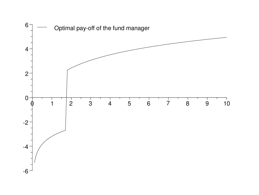
Figure 1: Optimal pay-off of the fund manager as function of the stock price value $S_{T}$.

Figure 2: Value function of Problem $\mathcal{P}_{1}$ as function of $c$.

Figure 3: The gain obtained by allowing a risk tolerance. The solid curve shows the optimal pay-off for the investor as in (1.1) and the dotted curve the optimal one when no risk is allowed: $\max\mathbb{E}\left[1-e^{-\delta X^{+}}\right]$ under $\mathbb{E}\left[\xi X\right]=x_{0}$ and $X\geq 0$.

4 Example: $CVaR$ and spectral risk measures

The $CVaR_{\beta}$ is a coherent risk measure defined by

$$CVaR_{\beta}\left(X\right):=\frac{1}{\beta}\int_{0}^{\beta}VaR_{u}\left(X\right)du=-\frac{1}{\beta}\int_{0}^{\beta}F^{-1}_{X}(u)du,$$ (4.1)

where $F^{-1}_{X}$ is a generalized inverse distribution function of $X$. Since the generalized inverse distribution function has at most a countable number of discontinuities, this definition does not depend on the particular choice of this function (right-continuous or left-continuous). In this section we shall always use the definition

$$F_{X}^{-1}(u):=\inf\{x:F(x)\geq u\}$$ (4.2)

with the convention $\inf\emptyset=+\infty$.

The $CVaR$ is the building block for a wide class of coherent risk measures called spectral risk measures. Given a probability measure $\mu$ on $\left[0,1\right]$, the spectral risk measure $\rho_{\mu}$ is defined by

$$\rho_{\mu}\left(X\right):=\int_{0}^{1}CVaR_{u}\left(X\right)\mu\left(du\right)=\int_{0}^{1}\phi\left(u\right)VaR_{u}\left(X\right)du$$ (4.3)

where

$$\phi\left(x\right):=\int_{x}^{1}\frac{\mu\left(ds\right)}{s}$$ (4.4)

The function $\phi$ is right-continuous, nonincreasing and by Fubini’s Theorem, $\int_{0}^{1}\phi\left(x\right)dx=1$. The case $\mu\left(du\right)=\delta_{\beta}\left(du\right)$ corresponds to $CVaR_{\beta}$. The function $\phi$ completely characterizes the spectral risk measure $\rho_{\mu}$.

In this section, we solve the portfolio optimization problem when the risk constraint is given by a spectral risk measure. We first need to compute the mappings $A\to\triangle\left(\mathit{A}\right)$ and $c\mapsto\Delta(c)$.

Lemma 4.1.

For $A\in\mathcal{F}$ with $\mathbb{P}\left(A\right)<1$, let $\hat{F}_{\xi}$ be the conditional distribution of $\xi$ on $A^{c}$ and define $\alpha_{A}:=\mathbb{P}\left(A^{c}\right)$. $\triangle\left(\mathit{A}\right)<-\infty$ if and only if

$$\lim_{x\rightarrow 0^{+}}\frac{\hat{F}_{\xi}^{-1}\left(1-x\right)}{\phi\left(x\right)}<+\infty$$ (4.5)

In this case

$$\triangle\left(\mathit{A}\right) = -\rho_{0}\max_{x\in\left[0,1\right]}r\left(x\right)$$ (4.6)

$$r\left(x\right) := \frac{\alpha_{A}}{\int_{0}^{\alpha_{A}x}\phi\left(u\right)du}\int_{0}^{x}\hat{F}_{\xi}^{-1}\left(1-u\right)du$$ (4.7)

Corollary 4.1.

The function $\Delta(c)$ is given by

$$\Delta(c)=-\rho_{0}\max_{0\leq z\leq\alpha(c)}R(z),\quad R(z):=\frac{\mathbb{E}\left[\xi\textbf{1}_{\left\{1-F_{\xi}(\xi)<z\right\}}\right]}{\int_{0}^{z}\phi\left(u\right)du}$$

Assume that the limit

$$\lim_{x\rightarrow 0^{+}}\frac{F_{\xi}^{-1}\left(1-x\right)}{\phi\left(x\right)}$$ (4.8)

exists. Then

$$\lim_{c\uparrow\overline{\xi}}\Delta(c)=-\rho_{0}\frac{F_{\xi}^{-1}\left(1-x\right)}{\phi\left(x\right)}.$$

The following theorem, which is the main result of this section, characterizes the solution of the problem (2.1) when the risk constraint is given by a spectral risk measure via a one-dimensional optimization problem.

Theorem 4.1.

Assume that there exists $c^{*}$ with $\mathbb{P}[\xi>c^{*}]>0$ such that $v(c^{*})=\max_{\underline{\xi}\leq c\leq\overline{\xi}}v(c)$ with

$$v(c)=\mathbb{E}[u(I(\lambda(c)\xi))\mathbf{1}_{\xi\leq c}],$$

where $\lambda(c)$ is the solution of

$$\mathbb{E}[\xi I(\lambda(c)\xi)\mathbf{1}_{\xi\leq c}]=x_{0}+\frac{\rho_{0}\mathbb{E}[\xi\mathbf{1}_{\xi>c}]}{\int_{0}^{\mathbb{P}[\xi>c]}\phi(u)du}.$$

Then the solution to the problem (2.1) is given by

$$X^{*}=I(\lambda(c^{*})\xi)\mathbf{1}_{\xi\leq c^{*}}-\frac{\rho_{0}}{\int_{0}^{\mathbb{P}[\xi>c^{*}]}\phi(u)du}\mathbf{1}_{\xi>c^{*}}.$$

Remark 4.1.

If $\sup_{\underline{\xi}\leq c\leq\overline{\xi}}v(c)$ is attained only by $c^{*}=\overline{\xi}$ and

$$\lim_{c\to\overline{\xi}}\frac{\mathbb{E}[\xi\mathbf{1}_{\xi>c}]}{\int_{0}^{\mathbb{P}[\xi>c]}\phi(u)du}<\infty,$$

(the latter condition holds, in particular, if $\overline{\xi}<\infty$), then $\inf_{A\in\mathcal{F}}\Delta(A)>-\infty$ but this infimum is not achieved: the extra gain from allowing a risk tolerance is bounded, but the optimal claim does not exist. Intuitively, claims which are “almost optimal” will lead to a very large loss occurring with a very small probability.

If

$$\limsup_{c\to\overline{\xi}}\frac{\mathbb{E}[\xi\mathbf{1}_{\xi>c}]}{\int_{0}^{\mathbb{P}[\xi>c]}\phi(u)du}=\infty$$

then $\inf_{A\in\mathcal{F}}\Delta(A)=-\infty$: the extra gain from allowing a risk tolerance is unbounded.

The special case: $CVaR_{\beta}$

In this case, $\mu\left(du\right)=\delta_{\beta}\left(du\right)$ and $\phi_{\beta}\left(x\right):=\frac{1}{\beta}\textbf{1}_{\left\{\beta>x\right\}}$, and the limit appearing in Condition (4.5) in Lemma 4.1 becomes

$$\lim_{x\to 0^{+}}\beta\hat{F}_{\xi}^{-1}(1-x)=\beta\overline{\xi}$$

Corollary 4.1, Lemma 2.1 and Theorems 2.3 and 4.1 enable us to give the solution of Problem (2.1):

• If $\bar{\xi}:=\mathrm{essup}\,\xi(\omega)<\infty$, then the value function of problem (2.1) is:

  $$\sup_{X\in H}U\left(X\right)=\sup_{c\in\left[\underline{\xi},\,\overline{\xi}\right]}\mathbb{E}\left[u\left(I\left(\lambda\left(c\right)\xi\right)\right)\mathbf{1}_{\left\{\xi\leq c\right\}}\right]$$ (4.9)

  where $\lambda\left(c\right)$ is the unique solution of

  $$\mathbb{E}\left[\xi I\left(\lambda\left(c\right)\xi\right)\mathbf{1}_{\left\{\xi\leq c\right\}}\right]=x_{0}+\rho_{0}\frac{\mathbb{E}[\xi\mathbf{1}_{\{\xi>c\}}]}{1\wedge\frac{\alpha(c)}{\beta}}$$

• If $\bar{\xi}=+\infty$ then there exists $A\in\mathcal{F}$ with $\triangle\left(\mathit{A}\right)=-\infty$.

The maximum in (4.9) is always attained for some $c^{*}\in[\underline{\xi},\,\overline{\xi}]$ because the value function is continuous and $[\underline{\xi},\overline{\xi}]$ is compact. If $c^{*}<\overline{\xi}$ then Theorem 4.1 applies and then we have a optimal solution for Problem (2.1). If the maximum is attained at $c^{*}=\overline{\xi}$, then, as in Remark 4.1, the optimal claim does not exist.

Remark 4.2.

From Theorem $4.47$ in Föllmer and Schied (2004), the minimal penalty function for the $CVAR_{\beta}$ is given by:

$$\gamma_{min}\left(\mathbb{Q}\right):=\left\{\begin{array}[]{ll}0&\textrm{if }\frac{d\mathbb{Q}}{d\mathbb{P}}\leq\frac{1}{\beta},\quad\mathbb{P}\textrm{-a.s}\\ +\infty&\textrm{otherwise}\end{array}\right.$$

If $\xi$ is bounded but $\mathbb{P}\left(\xi>\frac{1}{\beta}\right)>0$ then $\gamma_{min}\left(\xi\mathbb{P}\right)=+\infty$ and we have an example of a situation where Assumption (2.11) holds but the stronger assumption (2.12) fails.

5 Proofs

5.1 Proof of Lemma 2.1

Introduce the new probability space $\left(A,\mathcal{F}_{A}:=\{B\cap A,B\in\mathcal{F}\},\mathbb{P}\left(\cdot\left|\right.A\right)\right)$ and let $\mathbb{E}_{A}$ denote the expectation under the conditional probability $\mathbb{P}\left(\cdot\left|\right.A\right)$. The maximizer of $\mathcal{P}_{1}$, if it exists, is given by

$$Z\left(A,x^{+}\right)=W\left(A,x^{+}\right)\textbf{1}_{A}$$

where $W(A,x^{+})$ is the maximizer of the following problem on the new probability space:

$$\sup_{W\geq 0}\mathbb{E}_{A}\left[u\left(W\right)\right]$$

$$\textrm{subject to }\mathbb{E}_{A}\left[\xi W\right]=\frac{x^{+}}{\mathbb{P}\left(A\right)}.$$

This is a classical problem of maximizing a concave function under a linear constraint which can be solved by Lagrangian methods (see e.g., Karatzas and Shreve (1998)). First, $v$ is continuously differentiable, and since the mapping $\lambda\mapsto\mathbb{E}[v(\lambda\xi)]$ is convex and finite for all $\lambda$, it is differentiable, and using Fatou’s lemma we get that $\mathbb{E}[\xi v^{\prime}(\lambda\xi)]=\mathbb{E}\left[\xi I\left(\lambda\xi\right)\right]<+\infty$ for all $\lambda>0$. Therefore, the solution to the above optimization problem is

$$W\left(A,x^{+}\right)=I\left(\lambda\left(A,x^{+}\right)\xi\right)$$

where $\lambda\left(A,x^{+}\right)$ is the unique solution of $\mathbb{E}_{A}\left[\xi I\left(\lambda\xi\right)\right]=\frac{x^{+}}{\mathbb{P}\left(A\right)}$.

To show that $x^{+}\mapsto U\left(A,x^{+}\right)$ is strictly increasing, let $x_{1}^{+}<x^{+}_{2}$. Then the random variable

$$X=I\left(\lambda\left(A,x_{1}^{+}\right)\xi\right)\textbf{1}_{A}+\frac{x^{+}_{2}-x_{1}^{+}}{\mathbb{E}\left[\xi\textbf{1}_{A}\right]}$$

belongs to $\mathcal{H}_{1}\left(A,x_{2}^{+}\right)$, which proves that $U\left(A,x^{+}_{1}\right)<U\left(A,x^{+}_{2}\right)$.

The continuity of $U$ follows from inequality

$$u(I(\lambda\xi))\leq v(\xi)+\xi I(\lambda\xi)$$ (5.1)

and the continuity of $x^{+}\mapsto\lambda(A,x^{+})$, which is straightforward since the function $\lambda\mapsto\mathbb{E}[\xi I(\lambda\xi)\mathbf{1}_{A}]$ is strictly decreasing and continuous. The upper bound on $U$ is also a consequence of (5.1), after taking expectations.

5.2 Proof of Proposition 2.1

By definition of $\gamma_{min}$,

$$\gamma_{min}\left(\xi\mathbb{P}\right) =\sup_{Y\in\mathcal{A}_{\rho}}\mathbb{E}\left[-\xi Y\right]$$

$$=\sup_{Y+\rho_{0}\in\mathcal{A}_{\rho}}\mathbb{E}\left[-\xi Y\right]-\rho_{0}$$

$$\geq\sup_{Y+\rho_{0}\in\mathcal{A}_{\rho},Y\leq 0}\mathbb{E}\left[-\xi Y\right]-\rho_{0}$$

$$\geq\sup_{Y+\rho_{0}\in\mathcal{A}_{\rho},\ Y\leq 0,\ Y=0\ \text{on}\ A}\mathbb{E}\left[-\xi Y\right]-\rho_{0}$$

$$=\sup_{Y\in\mathcal{H}_{2}(A)}\mathbb{E}\left[-\xi Y\right]-\rho_{0}=-\triangle\left(\mathit{A}\right)-\rho_{0},$$

from which the result follows.

5.3 Proof of Theorem 2.1

Let us first prove (2.13). We start with the inequality “$\leq$”. Let $X^{n}\in H$ such that $U\left(X^{n}\right)\uparrow\sup_{X\in H}U\left(X\right)$. Define $A_{n}:=\left\{X^{n}\geq 0\right\}$ and $x_{n}:=\mathbb{E}\left[\xi X^{n}\textbf{1}_{A_{n}}\right]$.
One has then

$$U\left(X^{n}\right) = U\left(X^{n}\textbf{1}_{\mathit{A}^{n}}\right)$$

$$\leq U\left(\mathit{A}^{n},x_{n}\right)$$

$$\leq U\left(\mathit{A}^{n},x_{+}\left(\mathit{A}_{n}\right)\right)$$

$$\leq \sup_{A\in\mathcal{F}}U\left(\mathit{A},x_{+}\left(\mathit{A}\right)\right),$$

The first inequality holds because $X^{n}\textbf{1}_{\mathit{A}^{n}}\in\mathcal{H}_{1}\left(A_{n},x_{n}\right)$ and $U(A^{n},x_{n})$ is the sup over $\mathcal{H}_{1}\left(A_{n},x_{n}\right)$. The second inequality follows from the fact that $U(A,x^{+})$ is nondecreasing in $x^{+}$ provided we can prove that $x_{n}\leq x_{+}\left(\mathit{A}_{n}\right)=x_{0}-\triangle\left(\mathit{A}_{n}\right)$. Let $Y^{n}:=X^{n}-X^{n}\textbf{1}_{\mathit{A}_{n}}$, then $Y^{n}\in\mathcal{H}_{2}\left(A_{n}\right)$ and then

$$\mathbb{E}\left[\xi Y^{n}\right]\geq\inf_{Y\in\mathcal{H}_{2}\left(A_{n}\right)}\mathbb{E}\left[\xi Y\right]$$

which means

$$x_{0}-x_{n}\geq\triangle\left(A_{n}\right)=x_{0}-x^{+}\left(A_{n}\right)$$

i.e. $x_{n}\leq x^{+}\left(A_{n}\right)$

Let us now focus on the inequality “$\geq$”. Let $A_{n}\in\mathcal{F}$ be such that

$$U\left(\mathit{A}_{n},x_{+}\left(\mathit{A}_{n}\right)\right)\uparrow\sup_{A\in\mathcal{F}}U\left(\mathit{A},x_{+}\left(\mathit{A}\right)\right):=S,\,n\rightarrow+\infty$$

By the assumption of the theorem, $x^{+}(A_{n})<\infty$ for all $n$. Fix $\varepsilon>0$. Our aim is to find, for every $n$, $X_{n}\in H$ such that

$$U(X_{n})\geq U\left(\mathit{A}_{n},x_{+}\left(\mathit{A}_{n}\right)\right)-\varepsilon$$ (5.2)

Since $\varepsilon$ is arbitrary it will then follow that $\sup_{X\in H}U(X)\geq S$. If $P(A_{n})>0$, by Lemma 2.1 there exists an explicit maximizer of Problem $\mathcal{P}_{1}$, denoted by $Z(A_{n},x^{+})$, and $U(A_{n},x^{+})=U(Z(A_{n},x^{+}))$ is continuous in $x^{+}$. Therefore, we can find $Y_{n}\in\mathcal{H}_{2}(A_{n})$ with $\mathbb{E}[\xi Y_{n}]$ sufficiently close to $\triangle(A_{n})$ so that $U(A_{n},x_{0}-\mathbb{E}[\xi Y_{n}])\geq U(A_{n},x^{+}(A_{n}))-\varepsilon$. Then $X_{n}:=Z(A_{n},x_{0}-\mathbb{E}[\xi Y_{n}])+Y_{n}$ satisfies (5.2). If $P(A_{n})=0$ then, as we saw in Remark 2.1, taking $0\in H$ and $X_{n}=0$ satisfies $U(X_{n})=u(0)=U\left(\mathit{A}_{n},x_{+}\left(\mathit{A}_{n}\right)\right)$.

Finally, the fact that $S<\infty$ under Assumption (2.11) follows directly from the estimate (2.9).

5.4 Proof of Theorem 2.2

Let $X^{*}\in\mathit{H}$ be an optimal solution for (2.1), $A^{*}=\{X^{*}\geq 0\}$ and $Y^{*}=X^{*}\mathbf{1}_{X^{*}<0}$. It is clear that $Y^{*}\in\mathcal{H}_{2}\left(A^{*}\right)$. It is also clear that $\mathbb{P}(A)>0$, since otherwise $\mathbb{E}[\xi X^{*}]<x_{0}$ and one can increase the utility and reduce the risk by increasing $X^{*}$. Theorem 2.1 and the fact that $U(A,x^{+})$ is increasing in $x^{+}$ (Lemma 2.1) then give:

$$\sup_{A\in\mathcal{F}}U\left(A,x^{+}\left(A\right)\right) = \sup_{X\in H}U\left(X\right)$$

$$= U\left(X^{*}\right)$$

$$= U\left(X^{*}\textbf{1}_{A^{*}}\right)$$

$$= U\left(A^{*},x_{0}-\mathbb{E}[\xi Y^{*}]\right)$$

$$\leq U\left(A^{*},x^{+}\left(A^{*}\right)\right)$$

which means that $A^{*}$ achieves the supremum in (2.13). Moreover, since $U(A,x^{+})$ is strictly increasing in $x^{+}$, we get a contradiction unless $x^{+}(A^{*})=x_{0}-\mathbb{E}[\xi Y^{*}]$, which means that $Y^{*}$ achieves the minimum in $\mathcal{P}_{2}$.

Conversely, assume that $A^{*}$ is a maximizer of (2.13) and $Y^{*}$ is a minimizer of $\mathcal{P}_{2}$. We can then solve Problem $\mathcal{P}_{1}$ with parameters $(A^{*},x_{0}-\triangle(A^{*}))$ and we know, by Lemma 2.1, that its solution is given by $\left[I\left(\lambda^{*}\xi\right)^{+}\right]^{+}\textbf{1}_{A^{*}}$. Let then

$$X^{*}:=I\left(\lambda^{*}\xi\right)\textbf{1}_{A^{*}}+Y^{*}$$

We have $\rho\left(-(X^{*})^{-}\right)=\rho\left(Y^{*}\right)\leq\rho_{0}$ and $\mathbb{E}\left[\xi X^{*}\right]\leq x_{0}$, i.e. $X^{*}\in\mathit{H}$. Using Theorem 2.2, we deduce

$$U\left(X^{*}\right) = U\left(X^{*}\textbf{1}_{A^{*}}\right)$$

$$= U\left(A^{*},x^{+}\left(A^{*}\right)\right)$$

$$= \sup_{A\in\mathcal{F}}U\left(A,x^{+}\left(A\right)\right)$$

$$= \sup_{X\in\mathit{H}}U\left(X\right).$$

5.5 Proof of Theorem 2.3

We will use the methods developed in Jin and Zhou (2008) (see the proof of Theorem $5.1$). There are however some important differences in our proof which arise in particular due to the presence of risk measures in our context.

The theorem will be proved in two steps: in Step 1 we will prove that for every $A\in\mathcal{F}$, there exists $c\geq 0$ such that $\triangle\left(\mathit{A}\right)\geq\triangle\left(c\right):=\triangle\left(\left\{\xi\leq c\right\}\right)$ so that $x_{+}\left(c\right):=x_{0}-\triangle\left(\left\{\xi\leq c\right\}\right)\geq x_{+}\left(\mathit{A}\right)$, and in Step 2 we will find, for every $X\in\mathcal{H}_{1}\left(A,x^{+}\right)$, an $\hat{X}\in\mathcal{H}_{1}\left(\left\{\xi\leq c\right\},x^{+}\left(c\right)\right)$ such that $U\left(\hat{X}\right)\geq U\left(X\right)$. We can then conclude that $v\left(c\right):=v\left(\left\{\xi\leq c\right\}\right)\geq v\left(\mathit{A}\right)$

Treating separately the trivial cases as described in Remark 2.1, we can assume $0<\mathbb{P}\left(\mathit{A}\right)<1$, and set $\alpha=\mathbb{P}(A^{c})=1-\mathbb{P}(A)$. Let us fix $c\in\left[\underline{\xi},\overline{\xi}\right]$ so that

$$\mathbb{P}\left(\xi\leq c\right)=1-\alpha$$

This is possible since $\xi$ has no atom. Consider the following sets:

$$\mathit{A}_{1}=\left\{\xi\leq c\right\}\cap\mathit{A} \mathit{A}_{2}=\left\{\xi>c\right\}\cap\mathit{A}$$ (5.3)

$$\mathit{B}_{1}=\left\{\xi\leq c\right\}\cap\mathit{A}^{c} \mathit{B}_{2}=\left\{\xi>c\right\}\cap\mathit{A}^{c}$$ (5.4)

from which it follows $\mathbb{P}\left(\mathit{A}_{2}\right)=\mathbb{P}\left(\mathit{B}_{1}\right)$. If $\mathbb{P}\left(\mathit{A}_{2}\right)=0$ then $\mathit{A}=\left\{\xi\leq c\right\}$, so we can suppose $\mathbb{P}\left(\mathit{A}_{2}\right)>0$.
Step 1. Let $Y\in\mathcal{H}_{2}(A)$. Our aim is to construct $\hat{Y}\in\mathcal{H}_{2}(\{\xi\leq c\})$ with $\mathbb{E}[\xi\hat{Y}]=\mathbb{E}[\xi Y]$ and $\rho(Y)\geq\rho(\hat{Y})$. This will imply that $\triangle\left(\mathit{A}\right))\geq\triangle(c)$. Introduce the following notation:

1. $f_{1}\left(t\right):=\mathbb{P}\left(Y\leq t|\mathit{B}_{1}\right)$

2. $g_{1}\left(t\right):=\mathbb{P}\left(\xi\leq t|\mathit{A}_{2}\right)$

3. $Z_{1}=g_{1}\left(\xi\right)$, that is, $\mathcal{L}\left(Z_{1}|\mathit{A}_{2}\right)=\mathcal{U}(\left[0,1\right])$, because $\xi$ has no atom.

4. $W_{1}=f_{1}^{-1}\left(Z_{1}\right)$, that is, the law of $W$ on $A_{2}$ is the same as the law of $Y$ on $B_{1}$.

Let

$$k_{1}:=\left\{\begin{array}[]{ll}1&\textrm{if $W_{1}=0$ on $\mathit{A}_{2}$}\\ \\[3.0pt] \frac{{\mathbb{E}}\left[\xi Y\textbf{1}_{B_{1}}\right]}{{\mathbb{E}}\left[\xi W_{1}\textbf{1}_{A_{2}}\right]}&\textrm{otherwise}\\ \end{array}\right.$$

Observe that since $\xi\leq c$ on $B_{1}$, and $\xi>c$ on $A_{2}$, we have that $k\leq 1$. Now define

$$\hat{Y}=Y\mathbf{1}_{B_{2}}+kW_{1}\mathbf{1}_{A_{2}}.$$

By definition, $\hat{Y}=0$ on $\{\xi\leq c\}$ and $\hat{Y}\leq 0$ on $\{\xi\leq c\}$. In addition, since $k_{1}\leq 1$, we easily get that $\mathbb{P}(-\hat{Y}>t)\leq\mathbb{P}(-Y>t)$ for every $t>0$.

Let $F$ and $\hat{F}$ be the distribution functions of, respectively, $-Y$ and $-\hat{Y}$, and $F^{-1}$ and $\hat{F}^{-1}$ their generalized inverses (defined in (4.2)). From the above inequality, they satisfy $\hat{F}^{-1}(u)\leq F^{-1}(u)$ for all $u\in[0,1]$. Let $U$ be a random variable with uniform distribution on $[0,1]$. Since $\rho$ is law invariant, we obtain that $\rho(\hat{Y})=\rho(-\hat{F}^{-1}(U))\leq\rho(-\hat{F}^{-1}(U))=\rho(Y)\leq\rho_{0}$ and therefore $\hat{Y}\in\mathcal{H}_{2}(\{\xi\leq c\})$. On the other hand, $\mathbb{E}[\xi\hat{Y}]=\mathbb{E}[\xi Y]$ (this is due to our choice of the constant $k$). Since the choice of $Y$ was arbitrary, this means that $\triangle\left(\mathit{A}\right)\geq\triangle(c)$.

Step 2. Let $X$ be feasible for $\mathcal{P}_{1}$ with parameter $\left(\mathit{A},x_{+}\left(\mathit{A}\right)\right)$, and define

1. $f_{2}\left(t\right):=\mathbb{P}\left(X\leq t|\mathit{A}_{2}\right)$

2. $g_{2}\left(t\right):=\mathbb{P}\left(\xi\leq t|\mathit{B}_{1}\right)$

3. $Z_{2}=g_{2}\left(\xi\right)$

4. $W_{2}=f_{2}^{-1}\left(Z_{2}\right)$, that is, the law of $W_{2}$ on $B_{1}$ is the same as the law of $X$ on $A_{2}$.

Let

$$k_{2}:=\left\{\begin{array}[]{cc}1&\textrm{if $W_{2}=0$ on $\mathit{B}_{1}$}\\ \frac{\mathbb{E}\left[\xi X\textbf{1}_{\mathit{A}_{2}}\right]}{\mathbb{E}\left[\xi W_{2}\textbf{1}_{\mathit{B}_{1}}\right]}&\textrm{otherwise}\end{array}\right.$$

Note that now, $k_{2}\geq 1$. We define a new random variable $\hat{X}$ by

$$\hat{X}:=X\textbf{1}_{\mathit{A}_{1}}+k_{2}W_{2}\textbf{1}_{\mathit{B}_{1}}+\frac{x_{+}\left(c\right)-x^{+}\left(A\right)}{\mathbb{E}\left[\xi\textbf{1}_{\left\{\xi\leq c\right\}}\right]}\textbf{1}_{\left\{\xi\leq c\right\}}$$ (5.5)

We have $\mathbb{E}\left[\xi\hat{X}\right]=x^{+}\left(c\right)$ and it is easy to see that $\hat{X}\in\mathcal{H}_{1}\left(\left\{\xi\leq c\right\},x^{+}\left(c\right)\right)$. Moreover, since $k_{2}\geq 1$, a simple computation shows that

$$\mathbb{P}\left(\hat{W}>t\right)\geq\mathbb{P}\left(X>t\right)$$

By definition,

$$U\left(X\right)=\mathbb{E}\left[u\left(X^{+}\right)\right]=\int^{+\infty}_{0}\mathbb{P}\left(X^{+}>u^{-1}\left(t\right)\right)dt$$ (5.6)

$$U\left(\hat{W}\right)=\mathbb{E}\left[u\left(\hat{W}^{+}\right)\right]=\int^{+\infty}_{0}\mathbb{P}\left(\hat{W}^{+}>u^{-1}\left(t\right)\right)dt$$

but since $u^{-1}\left(t\right)$ is positive,

$$\left\{\hat{W}^{+}>u^{-1}\left(t\right)\right\}=\left\{\hat{W}>u^{-1}\left(t\right)\right\}$$

$$\left\{X^{+}>u^{-1}\left(t\right)\right\}=\left\{X>u^{-1}\left(t\right)\right\},$$

which enables us to conclude that $U\left(X\right)\leq U\left(\hat{X}\right)$.

5.6 Proof of Theorem 3.1

Proof.

The proof is just a simple application of Theorems 2.2, 2.3, Lemma 2.1 and Lagrangian methods.

Fix $c$ and consider the problem:

$$\left\{\begin{array}[]{ll}\inf\mathbb{E}\left[\xi Y\right]&\textrm{s.t.}\\ \rho\left(Y\right)\leq\rho_{0}&\\ Y=0\quad\textrm{on $\mathit{A}$},\quad Y\leq 0\quad\textrm{on $\mathit{A}^{c}$}&\textrm{and}\\ \end{array}\right.$$

where $\mathit{A}=\left\{\xi\leq c\right\}$
Working on the new space $\left({A}^{c},\hat{\mathcal{F}}:=\{B\cap A^{c},B\in\mathcal{F}\},\hat{\mathbb{P}}:=\mathbb{P}(\cdot|A^{c})\right)$, we can transform this minimization into

$$\left\{\begin{array}[]{cc}\inf\alpha\left(c\right)\hat{\mathbb{E}}\left[\xi W\right]&\textrm{s.t.}\\ \\[4.0pt] \hat{\mathbb{E}}\left[\exp\left(-\frac{W}{\beta}\right)\right]\leq\delta\left(c\right),&W\leq 0\\ \end{array}\right.$$

where

$$\delta\left(c\right)=\frac{e^{\frac{\rho_{0}}{\beta}}+\alpha\left(c\right)-1}{\alpha\left(c\right)}.$$

Using Lagrangian methods we can find the unique optimal solution:

$$W^{*}\left(c\right):=-\beta\left[\log\left(\frac{\beta}{\eta\left(c\right)}\xi\right)\right]^{+}$$

where $\eta\left(c\right)$ is the unique solution of:

$$\mathbb{E}\left[\left(\frac{\beta\xi}{\eta(c)}\vee 1\right)\mathbf{1}_{\xi>c}\right]=e^{\frac{\rho_{0}}{\beta}}+\alpha(c)-1,$$

and so

$$Y^{*}\left(c\right):=W^{*}\left(c\right)\textbf{1}_{\left\{\xi>c\right\}}.$$

A simple calculation then gives:

$$\triangle\left(c\right)=-\beta\mathbb{E}\left[\xi\log\left(\frac{\beta\xi}{\eta(c)}\vee 1\right)\right].$$

If now we set $x_{+}\left(c\right)=x_{0}-\triangle\left(c\right)$, by Lemma 2.1 , Problem $\mathcal{P}_{1}$ with parameters $\left(\left\{\xi\leq c\right\},x^{+}\left(c\right)\right)$ can be solved and its unique solution is

$$X\left(c\right)=I\left(\lambda\left(c\right)\xi\right)\textbf{1}_{\left\{\xi\leq c\right\}},$$

where, by (2.8),

$$\mathbb{E}\left[\xi I\left(\lambda\left(c\right)\xi\right)\textbf{1}_{\left\{\xi\leq c\right\}}\right]=x^{+}\left(c\right).$$

Using Theorem 2.3, the optimal $c^{*}$ is the maximizer of the function

$$c\rightarrow\mathbb{E}\left[u\left(I\left(\lambda\left(c\right)\xi\right)\right)\textbf{1}_{\left\{\xi\leq c\right\}}\right].$$

∎

5.7 Proof of Lemma 4.1

Proof.

In order to compute $\triangle\left(\mathit{A}\right)$ we reformulate Problem $\mathcal{P}_{2}$ in terms of the conditional distribution function of $Y\in\mathcal{H}_{2}\left(A\right)$ on $A^{c}$. Introduce a new probability $\hat{\mathbb{P}}$ via $\frac{d\hat{\mathbb{P}}}{d{\mathbb{P}}}=\frac{\mathbf{1}_{A^{c}}}{\alpha_{A}}$. Let $\hat{F}_{Y}$ be the distribution function of $Y$ under this probability and $\hat{F}_{Y}^{-1}$ its generalized inverse. Using this new probability we can rewrite the ingredients of our problem as

$$\mathbb{E}[\xi Y]=\alpha_{A}\hat{\mathbb{E}}[\xi Y]$$

and

$$CVAR_{\beta}(Y) =-\frac{1}{\beta}\int_{0}^{\beta}F^{-1}_{Y}(u)=-\frac{1}{\beta}\int_{0}^{\beta\wedge\alpha_{A}}\hat{F}^{-1}_{Y}(u/\alpha_{A})du$$

$$=-\frac{\alpha_{A}}{\beta}\int_{0}^{\frac{\beta}{\alpha_{A}}\wedge 1}\hat{F}^{-1}_{Y}(u)du.$$

and then using (4.3) we obtain

$$\rho_{\mu}(Y) =-\alpha_{A}\int_{0}^{1}\phi\left(\alpha_{A}u\right)\hat{F}^{-1}_{Y}(u)du.$$

To express $\hat{\mathbb{E}}[\xi Y]$, we use the following well known result:

Lemma 5.1.

Let $F_{1}$ and $F_{2}$ be distribution functions on $[0,\infty)$. Then

$$\sup_{X\sim F_{1},\ Y\sim F_{2}}\mathbb{E}[XY]=\int_{0}^{1}F_{1}^{-1}(u)F_{2}^{-1}(u)du.$$

Using this lemma, Problem $\mathcal{P}_{2}$ can be expressed as

$$\triangle\left(\mathit{A}\right)=\alpha_{A}\inf\int_{0}^{1}\hat{F}^{-1}_{\xi}(u)\hat{F}^{-1}_{Y}(1-u)du$$ (5.7)

$$\text{subject to}\quad-\alpha_{A}\int_{0}^{1}\phi\left(\alpha_{A}u\right)\hat{F}^{-1}_{Y}(u)du\leq\rho_{0},$$ (5.8)

where the $\inf$ is taken over all generalized inverse distribution functions $\hat{F}^{-1}_{Y}$ of non-positive random variables. Such a function can always be written as

$$\hat{F}^{-1}_{Y}\left(u\right):=-\int_{u}^{1}\zeta\left(du\right),$$ (5.9)

where $\zeta$ is a positive measure on $[0,1]$. Using Fubini’s theorem, we can rewrite problem (5.7)–(5.8) in terms of this measure:

$$\triangle\left(\mathit{A}\right)=-\alpha_{A}\sup\left(\int_{0}^{1}\zeta(ds)\int_{0}^{s}\hat{F}^{-1}_{\xi}(1-u)du\right)$$

$$\text{subject to}\quad\alpha_{A}\left(\int_{0}^{1}\zeta(ds)\int_{0}^{s}\phi\left(\alpha_{A}u\right)du\right)\leq\rho_{0}.$$

The solution of this problem can easily be shown to be a point mass: $\zeta=h\delta_{x}$ where $h\geq 0$ and $x\in[0,1]$ can be found from

$$\triangle\left(\mathit{A}\right)=-\alpha_{A}\sup\left(h\int_{0}^{x}\hat{F}^{-1}_{\xi}(1-u)du\right)$$ (5.10)

$$\text{subject to}\quad\alpha_{A}h\int_{0}^{x}\phi\left(\alpha_{A}u\right)du=\rho_{0},$$ (5.11)

The constraint (5.11) gives us

$$h=h\left(x\right)=\frac{\rho_{0}}{\alpha_{A}\int_{0}^{x}\phi\left(\alpha_{A}s\right)ds}$$

and using definition (4.7) we get

$$\triangle\left(\mathit{A}\right) = -\alpha_{A}\sup_{x\in[0,1]}\left(\frac{\rho_{0}}{\alpha_{A}\int_{0}^{x}\phi\left(\alpha_{A}s\right)ds}\int_{0}^{x}\hat{F}^{-1}_{\xi}(1-u)du\right)$$

$$= -\rho_{0}\sup_{x\in\left[0,1\right]}r\left(x\right)$$

The function $r$ is differentiable on $(0,1]$ and may only have a singularity at $x=0$; using l’Hôpital’s rule, we get

$$r\left(0^{+}\right)=\lim_{x\rightarrow 0}\frac{\hat{F}^{-1}_{\xi}(1-x)}{\phi\left(x\right)}$$

So $\triangle\left(\mathit{A}\right)<+\infty$ if and only if $r$ is bounded on $\left[0,1\right]$, which is true if and only if $r\left(0^{+}\right)<+\infty$. ∎

5.8 Proof of Corollary 4.1

Proof.

In order to make the dependence on $c$ explicit, we introduce the notation

$$\triangle\left(c\right):=-\rho_{0}\max_{x\in\left[0,1\right]}R\left(x,c\right)$$

where

$$R\left(x,c\right):=\frac{\alpha\left(c\right)\int_{0}^{x}\hat{F}^{-1}_{\xi}\left(1-u\right)du}{\int_{0}^{\alpha\left(c\right)x}\phi\left(u\right)du}$$

Noting that $\hat{F}_{\xi}^{-1}(1-u)=F^{-1}_{\xi}(1-\alpha(c)u)\geq c$ and making a change of variable,

$$R\left(x,c\right) =\frac{\mathbb{E}\left[\xi\textbf{1}_{\left\{c<\xi\right\}}\textbf{1}_{\left\{\hat{F}^{-1}_{\xi}\left(1-x\right)<\xi\right\}}\right]}{\int_{0}^{\alpha\left(c\right)x}\phi\left(u\right)du}=\frac{\mathbb{E}\left[\xi\textbf{1}_{\left\{c<\xi\right\}}\textbf{1}_{\left\{\hat{F}^{-1}_{\xi}\left(1-x\right)<\xi\right\}}\right]}{\int_{0}^{\alpha\left(c\right)x}\phi\left(u\right)du}$$

$$=\frac{\mathbb{E}\left[\xi\textbf{1}_{\left\{F^{-1}_{\xi}\left(1-\alpha(c)x\right)<\xi\right\}}\right]}{\int_{0}^{\alpha\left(c\right)x}\phi\left(u\right)du}=\frac{\mathbb{E}\left[\xi\textbf{1}_{\left\{1-F_{\xi}(\xi)<\alpha(c)x\right\}}\right]}{\int_{0}^{\alpha\left(c\right)x}\phi\left(u\right)du}$$

The function $\Delta(c)$ can then be rewritten as

$$\Delta(c)=-\rho_{0}\max_{0\leq z\leq\alpha(c)}R(z),\quad R(z):=\frac{\mathbb{E}\left[\xi\textbf{1}_{\left\{1-F_{\xi}(\xi)<z\right\}}\right]}{\int_{0}^{z}\phi\left(u\right)du}$$

∎

5.9 Proof of Theorem 4.1

Proof.

From Theorem 2.3 we need to maximize the function $c\mapsto v(c)$ over $c\in[\underline{\xi},\,\overline{\xi}]$. Assume that $v(c)$ achieves its maximum at the point $c^{*}$ such that $\Delta(c^{*})=-\rho R(z)$ with $z<\alpha(c)$ and let $c^{\prime}=\alpha^{-1}(z)$. Then, $\Delta(c)$ is constant on the interval $[c,c^{\prime}]$, which means that $x^{+}(c)=x^{+}(c^{\prime})$,

$$\mathcal{H}_{1}\left(\left\{\xi\leq c\right\},x^{+}(c)\right)\subset\mathcal{H}_{1}\left(\left\{\xi\leq c^{\prime}\right\},x^{+}(c^{\prime})\right)$$

and therefore $v(c)\leq v(c^{\prime})$. This argument shows that the solution of the optimization problem appearing in the right-hand side of (2.19) does not change if we replace the expression for $\Delta(c)$ given by Corollary 4.1 by

$$-\rho_{0}R(\alpha(c))=-\frac{\rho_{0}\mathbb{E}[\xi\mathbf{1}_{\xi>c}]}{\int_{0}^{\mathbb{P}[\xi>c]}\phi(u)du}.$$

Applying Lemma 2.1 we then find

$$v(c)=\mathbb{E}[u(I(\lambda(c)\xi))\mathbf{1}_{\xi\leq c}],$$

where

$$\mathbb{E}[\xi I(\lambda(c)\xi)\mathbf{1}_{\xi\leq c}]=x_{0}+\frac{\rho_{0}\mathbb{E}[\xi\mathbf{1}_{\xi>c}]}{\int_{0}^{\mathbb{P}[\xi>c]}\phi(u)du}.$$

If there exists a $c^{*}$ with $\mathbb{P}(\xi>c^{*})>0$ which maximizes the value function $c\to v(c)$ then the optimal contingent claim is given by

$$X^{*}=I(\lambda(c^{*})\xi)\mathbf{1}_{\xi\leq c^{*}}-\frac{\rho_{0}}{\int_{0}^{\mathbb{P}[\xi>c^{*}]}\phi(u)du}\mathbf{1}_{\xi>c^{*}}.$$

where

$$-\frac{\rho_{0}}{\int_{0}^{\mathbb{P}[\xi>c^{*}]}\phi(u)du}\mathbf{1}_{\xi>c^{*}}.$$

is the optimal solution of Problem $\mathcal{P}_{2}$ corresponding to $\left\{\xi\leq c^{*}\right\}$, which can be deduced from the proof of Lemma 4.1. ∎

References

- Biagini and Frittelli (2009) Biagini, S. and M. Frittelli (2009). On the extension of the Namioka-Klee theorem and on the Fatou property for risk measures. In Optimality and Risk — Modern Trends in Mathematical Finance, pp. 1–28. Springer.
- Black and Perold (1992) Black, F. and A. Perold (1992). Theory of constant proportion portfolio insurance. Journal of Economic Dynamics and Control 16(3-4), 403–426.
- Bouchard et al. (2010) Bouchard, B., R. Elie, and C. Imbert (2010). Optimal control under stochastic target constraints. SIAM Journal on Control and Optimization 48(5), 3501–3531.
- Bouchard et al. (2009) Bouchard, B., R. Elie, and N. Touzi (2009). Stochastic target problems with controlled loss. SIAM Journal on Control and Optimization 48, 3123–3150.
- Boyle and Tian (2007) Boyle, P. and W. Tian (2007). Portfolio management with constraints. Mathematical Finance 17(3), 319–343.
- Cont and Tankov (2009) Cont, R. and P. Tankov (2009). Constant proportion portfolio insurance in the presence of jumps in asset prices. Mathematical Finance 19(3), 379–401.
- El Karoui et al. (2005) El Karoui, N., M. Jeanblanc, and V. Lacoste (2005). Optimal portfolio management with American capital guarantee. Journal of Economic Dynamics and Control 29(3), 449–468.
- Emmer et al. (2001) Emmer, S., C. Klüppelberg, and R. Korn (2001). Optimal portfolios with bounded capital at risk. Mathematical Finance 11(4), 365–384.
- Föllmer and Leukert (1999) Föllmer, H. and P. Leukert (1999). Quantile hedging. Finance and Stochastics 3(3), 251–273.
- Föllmer and Schied (2004) Föllmer, H. and A. Schied (2004). Stochastic finance. An introduction in discrete time. de Gruyter Studies in Mathematics.
- Gundel and Weber (2007) Gundel, A. and S. Weber (2007). Robust utility maximization with limited downside risk in incomplete markets. Stochastic Processes and Their Applications 117(11), 1663–1688.
- He and Zhou (2010) He, X. D. and X. Y. Zhou (2010). Portfolio choice via quantiles. preprint.
- Jin and Zhou (2008) Jin, H. and Y. Zhou (2008). Behavioral portfolio selection in continuous time. Mathematical Finance 18(3), 385–426.
- Jouini et al. (2006) Jouini, E., W. Schachermayer, and N. Touzi (2006). Law invariant risk measures have the Fatou property. Advances in mathematical economics 9, 49–71.
- Kaina and Rüschendorf (2009) Kaina, M. and L. Rüschendorf (2009). On convex risk measures on -spaces. Mathematical Methods of Operations Research 69(3), 475–495.
- Karatzas and Shreve (1998) Karatzas, I. and S. Shreve (1998). Methods of mathematical finance. Springer Verlag.
- Rockafellar and Uryasev (2000) Rockafellar, R. and S. Uryasev (2000). Optimization of conditional value-at-risk. Journal of risk 2, 21–42.