Spin-Hall current and spin polarization in an electrically biased SNS Josephson junction

Abstract

Periodic in time spin-Hall current and spin polarization induced by a dc electric bias has been calculated in a superconductor-normal 2DEG-superconductor (SNS) Josephson junction. We assumed that the band energies of electrons in the normal system are splitted due to Rashba spin-orbit coupling. The transport parameters have been calculated within the diffusion approximation and using perturbation expansion over a small SN contact transparency. We found out that in contrast to the stationary Josephson effect, the spin-Hall current does not turn to zero. Besides a direct proximity effect caused by Cooper pair’s transition into a triplet state, the spin current and polarization are also driven by a periodic electric field associated with the charge imbalance.

I Introduction

The spin-Hall effect (SHE) is a fundamental physical phenomenon where the spin-orbit interaction (SOI) shows up in electron transport on a macroscopic level. The interplay of spin precession caused by SOI and electron acceleration in the electric field gives rise to a flux of the out-of-plane spin polarization flowing perpendicular to the electric current. Although this effect was predicted long time ago Dyakonov , it has been observed experimentally only recently in semiconductors Kato ; Wunderlich and metals Valenzuela . The nature of this phenomenon is now well understood and studied for various systems (for a review see Engel, ). The spin-Hall effect is being considered as a tool for manipulating electron spins in perspective spintronic applications. On the other hand, the spin polarization accumulated due to SHE is subject to dissipative processes of spin relaxation and diffusion. From this point of view, it is interesting to consider SHE in superconductors, as well as in SNS junctions, where the N-region is represented by a normal electron system with a strong enough spin-orbit coupling. Also, in such systems SHE provides an opportunity for a direct coupling of spin degrees of freedom to superconducting quibits quibits ; Schuster

An important distinction of spin-Hall effects in superconducting and normal systems is that in the latter case this effect is determined by spin dynamics of single particles, while in the former case major role is played by interference of triplet and singlet Cooper pairs MalshukovSNS . The triplet correlations, in their turn, are induced in the condensate wave function by SOI Gorkov , and shows up as admixture to the singlet state. Therefore, the spin current and spin accumulation caused by SHE are determined by a coherent macroscopic state and do not dissipate. SHE has been considered in bulk superconductors Contani and SNS tunneling contacts MalshukovSNS . Also in such contacts an effect reciprocal to SHE was recently studied MalshukovISNS . These studies have been restricted to the stationary transport. In the case of SNS junctions this means that the Josephson electric current is driven by a phase difference of superconducting order parameters of two superconducting electrodes. If these electrodes have different electric potentials, this current will periodically vary in time. One would expect that, due to such a time dependence, the non-zero spin-Hall current will be induced, while it is forbidden in the stationary case by the time inversion symmetry. MalshukovSNS One more nonstationary effect is associated with an electric field caused by a dynamic electron-hole charge imbalance within the normal layer. Such a periodic field will drive a flux of the spin polarization, in a way quite similar to conventional SHE in normal systems.

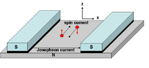
Figure 1: (Colour online) An SNS Josephson junction. The ac Josephson electric current flows in $x$-direction between two superconducting electrodes (blue) through normal 2DEG (gray). Black layers show tunneling barriers. In the presence of Rashba spin-orbit coupling the ac spin current of $z$-polarized electrons in $y$-direction is induced, with zero z-oriented spin density. A finite spin polarization in y-direction (not shown) is also induced .

The goal of the present study is to extend the theory of Ref.MalshukovSNS, to the case of the non-stationary Josephson effect. We will calculate the spin-Hall current and spin polarization created by a combined effects of the Josephson tunneling and SOI. It will be assumed that two singlet superconducting electrodes are under the dc electric voltage $V$. The normal layer is contacted to them through the low transparency tunneling barriers, as shown in Fig.1. This layer is taken thin enough, so that electrons are restricted to 2D motion, as, for example in a semiconductor quantum well. The spin-orbit coupling in the N-layer is given by the Rashba interaction RashbaSOI and we will ignore the spin-orbit effects in scattering of electrons from impurities. At the same time the spin-independent scattering will be taken into account within the Born approximation. The particle’s mean free path $l$ will be assumed smaller than all relevant parameters of length dimension, except the Fermi wavelength $k_{F}$, which in the semiclassical approximation is much smaller than $l$. Therefore, the electron transport within the N-layer is dominated by diffusion.

The outline of this paper is as follows. The general expressions for the spin-Hall current and spin density are derived in Sec. II. In Sec. III some numerical results are presented and discussed. Finally, Appendix A presents some details of analytical calculations within the Keldysh formalizm.

II Basic equations

Since we will focus on the basic characteristics of SHE, the simplest approach will be employed within the lowest-order perturbation theory with respect to transmission coefficients of interface barriers. It should be noted, however, that higher-order corrections to the electric Josephson current are not always small Feigelman , in particular in the range of temperatures $T$ larger than the Thouless energy $E_{Th}=D/L^{2}$, where $D$ is the diffusion constant and $L$ is the distance between contacts. We will assume the temperature or/and the transmission coefficient low enough to avoid such a situation. The tunneling is presented by the perturbation Hamiltonian

$$\hat{H}_{int}=\sum_{k,k^{\prime},\sigma}t_{k,k^{\prime}}\hat{a}^{{\dagger}}_{k^{\prime}\sigma}\tau_{3}\hat{c}_{k\sigma}+h.c.\,,$$ (1)

where $a_{k\sigma}$ and $c_{k\sigma}$ are electron destruction operators in the superconductor and N-layer, respectively, with $k$ denoting the wavevector and $\sigma$ the spin projection of the particles. The transmission coefficient will be assumed a slow varying function of wavevectors in the vicinity of the Fermi surface. Hamiltonian (1) is written in the Nambu representation, where destruction operators are defined as

$$\hat{c}_{k\sigma}=\left(\begin{array}[]{cc}c_{k\sigma}\\ c^{{\dagger}}_{-k\bar{\sigma}}\end{array}\right),$$ (2)

and $\tau_{1},\tau_{2},\tau_{3}$ are the Pauli matrices in the Nambu space. In its turn, the unperturbed Hamiltonian of the normal layer has the form

$$\hat{H}_{0} = \sum_{k,\sigma,\sigma^{\prime}}\hat{c}^{{\dagger}}_{k\sigma}\left(\frac{\delta_{\sigma\sigma^{\prime}}\hat{\tau_{3}}}{2m^{*}}k^{2}-\delta_{\sigma\sigma^{\prime}}\hat{\tau}_{3}\mu+\bm{\sigma}_{\sigma\sigma^{\prime}}\cdot\mathbf{h}_{\mathbf{k}}\right)\hat{c}_{k\sigma^{\prime}}+$$ (3)

$$\sum_{k,k^{\prime},\sigma}U_{k,k^{\prime}}\hat{c}^{{\dagger}}_{k^{\prime}\sigma}\tau_{3}\hat{c}_{k\sigma}+H_{c}\,,$$

where $\bm{\sigma}=(\sigma^{x},\sigma^{y},\sigma^{z})$ is the Pauli spin vector. The Rashba spin-orbit field $\mathbf{h}_{\mathbf{k}}$, which is the odd function of $\mathbf{k}$, is given by RashbaSOI $\hat{h}^{x}_{\mathbf{k}}=\alpha k_{y},\hat{h}^{y}_{\mathbf{k}}=-\alpha k_{x}$. The random impurity scattering potential is represented by its matrix elements $U_{k,k^{\prime}}$. This scattering determines the elastic mean free time $\tau$ of electrons. For a short-range scattering it is given by $1/\tau=2\pi N_{F}\langle|U_{k,k^{\prime}}|^{2}\rangle_{\text{imp}}=2\pi n_{i}N_{F}|U|^{2}$ , where $N_{F}$ is the state density at the Fermi level, $n_{i}$ is the impurity concentration and the subscript ”imp” denotes averaging over impurity positions. The Hamiltonian $H_{c}$ represents the Coulomb interaction of electrons. It will be treated within the random phase approximation to take into account screening effects associated with the dynamic charge imbalance, while its contribution to the self-energy and electron-electron correlations will be ignored.

We assume that SNS contact is unbounded in the $y$-direction. Hence, the Josephson current is in the $x$-direction, as shown in Fig. 1, and the spin-Hall current polarized parallel to the $z$-axis flows in the $y$-direction and depends on the $x$-coordinate. In the framework of the Keldysh formalism Landau it can be written as

$$J_{s}(x,t)=\frac{1}{4m^{*}}(\nabla_{y^{\prime}}-\nabla_{y})\mathrm{Tr}[\sigma^{z}\langle G^{K}_{11}(t,\mathbf{r};t,\mathbf{r}^{\prime})\rangle_{\text{imp}}]|_{\mathbf{r}\rightarrow\mathbf{r}^{\prime}}\,,$$ (4)

where $G^{K}_{11}(t,\mathbf{r};t,\mathbf{r}^{\prime})$ is a nondiagonal (Keldysh) component of the Green function, which is a 2$\times$2 matrix in the spin space, with subscript 11 denoting the corresponding projection in the Nambu space. Besides the spin current we will calculate also the spin polarization along the $y$-axis. In normal systems such a spin polarization is due to the electric spin orientation Edelstein . It is usually associated with SHE and takes place also at stationary Josephson tunneling conditions MalshukovSNS . This polarization can be expressed as

$$S_{y}(x,t)=-\frac{i}{2}\mathrm{Tr}[\sigma^{y}\langle G^{K}_{11}(t,\mathbf{r};t,\mathbf{r})\rangle_{\text{imp}}]$$ (5)

Expressions (4) and (5) have to be expanded up to the 4-th order with respect to the transmittance. The relevant diagrams are shown in Fig.2. Comparing them to a diagram representation of the charge Josephson current Aslamazov one can see that in the latter case diagrams are much simpler. That is because conservation of the Josephson current allows to reduce its calculation to calculation of the charge time derivative in one of the superconducting terminals. Unlike the Josephson current, the spin current does not conserve and such a simplification is not possible. An additional problem is caused by time dependence of the charge transport. It results in an electric potential inside the N-layer. Therefore, one should take into account diagrams which explicitly take into account the Coulomb screening there. These diagrams are shown in Fig. 3. The calculations below will be restricted to the low temperature $T$ and small enough DC voltage $V$, both much less than the superconducting gap $\Delta$. In this regime the electron transport through the contact will be dominated by tunneling of Cooper pairs between two superconducting electrodes, while a dissipative transport due to electronic excitations will be exponentially suppressed. Henceforth, the Green functions of superconductor terminals are represented in Fig. 2 and Fig. 3 by corresponding anomalous functions. More details on calculation of Feynman diagrams in Figs. 2 and 3 can be found in Appendix A.

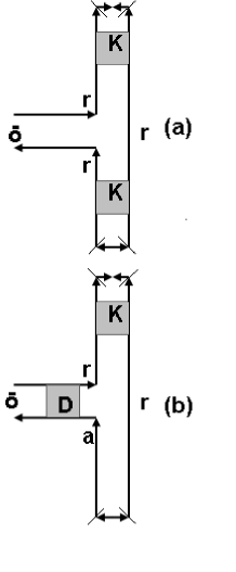
Figure 2: (Color online) Examples of Feynman diagrams for calculation of the spin current and spin polarization. The operator $\bar{\mathbf{O}}$ denotes the spin current, or spin density operators. Grey boxes are diffusion propagators. Boxes denoted by ”K” and ”D” relate to Cooperon and diffuson, respectively. ”r” and ”a” stand for retarded and advanced Green functions. Slashes denote the tunneling amplitude

The main building blocks of diagrams in Fig. 2 and Fig. 3 are unperturbed equilibrium Green functions averaged over impurity positions. For the normal layer these functions are determined by Hamiltonian (3) and are represented by their retarded ($r$), advanced ($a$) and Keldysh components

$$\hat{G}^{0r(a)}(\omega,\mathbf{k})=\left(\omega-\tau_{3}E_{k}-\bm{\sigma}\cdot\mathbf{h}_{\mathbf{k}}\pm i\Gamma\right)^{-1}\,,$$ (6)

where $E_{k}=(k^{2}/2m^{*})-\mu$ and $\Gamma=1/2\tau$,

$$\hat{G}^{0K}(\omega,\mathbf{k})=\tanh\frac{\omega}{2k_{B}T}\left(\hat{G}^{0r}(\omega,\mathbf{k})-\hat{G}^{0a}(\omega,\mathbf{k})\right)\,.$$ (7)

Important entries in Fig. 2 are the propagators $\mathrm{D}$ and $\mathrm{K}$ given by

$$D_{\alpha\beta\nu\mu}(\omega_{1}-\omega_{2})=$$

$$n_{i}|U|^{2}\langle G_{\alpha\mu;11}^{r}(\mathbf{r},\mathbf{r}^{\prime},\omega_{1})G_{\nu\beta;11}^{a}(\mathbf{r}^{\prime},\mathbf{r},\omega_{2})\rangle_{\text{imp}}$$ (8)

and

$$K_{\alpha\beta\nu\mu}^{r(a)}(\omega_{1}+\omega_{2})=$$

$$n_{i}|U|^{2}\langle G_{\alpha\mu;11}^{r(a)}(\mathbf{r},\mathbf{r}^{\prime},\omega_{1})G_{\nu\beta;22}^{r(a)}(\mathbf{r}^{\prime},\mathbf{r},\omega_{2})\rangle_{\text{imp}}.$$ (9)

The conjugated functions $\mathrm{K}^{{\dagger}}$ are defined by Eq. (II) with interchanged Nambu subscripts 11 and 22. Within the semiclassical approximation $\mathrm{D}$ and $\mathrm{K}$ can be represented by the ladder series. agd At small frequencies and large $|\mathbf{r}-\mathbf{r}^{\prime}|\gg l$ they satisfy a diffusion equation and are called ”diffuson” and ”Cooperon”, respectively. Altshuler Due to the time inversion symmetry these correlators are not independent. They can be expressed via each other.

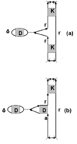
Figure 3: (Color online) Examples of Feynman diagrams for calculation of Coulomb screening effects on the spin current and spin polarization (see Fig. 2 for details). Dashed line denotes the screened Coulomb potential.

Depending on a combination of spin components, the diffuson and Cooperon describe either spin, or particle (charge) diffusion. Therefore, it is convenient to expand them in terms of Pauli matrices, according to

$$D_{\alpha\beta\nu\mu}=\frac{1}{2}D_{ij}\sigma^{i}_{\alpha\beta}\sigma^{j}_{\nu\mu}\,,$$ (10)

where $i,j=x,y,z,0$ and $\sigma^{0}$ denotes the 2$\times$2 unity matrix. Here and below a summation is assumed over the vector, or spinor indexes entering twice into an expression. Cooperon components can be represented in a way similar to (10). The tensor components $D_{ij}$ have a clear physical meaning. Namely, $D_{00}$ relates to the particle diffusion, while various components with $i,j=x,y,z$ are associated with the spin diffusion. Mixed terms, for example $D_{i0}$, are generally not zero in the presence of SOI. As follows from definitions (2) and (II), $z$-components of $\mathrm{K}$ are related to diffusion of singlet Cooper pairs, because they involve antisymmetric combinations of ”up” and ”down” spins in the particle-particle scattering process associated with the propagator $\mathrm{K}$. Other components, 0,x,y are related to triplet Cooperons. It is easy to see that the the 0-term gives a triplet with a 0 spin projection onto the $z$-axis, while $x$ and $y$ components are various combinations of $\pm 1$ triplets. A singlet-triplet mixing is associated with nondiagonal correlators $K_{zm},K_{mz}$, where $m=0,\pm 1$. As it will become clear below, the mixing terms are proportional to the small parameter $\alpha/v_{F}$, where $v_{F}$ is the Fermi velocity. Only linear in this parameter terms will be taken into account in the following calculations of the spin-Hall current and spin polarization.

Since $\mathrm{K}$ always enters together with the Green functions of superconducting terminals, it is convenient to introduce the pairing function

$$F^{r(a)}_{\alpha\beta}(\mathbf{r},\omega)=\int d^{2}r^{\prime}K^{r(a)}_{\alpha\beta\nu\mu}(\mathbf{r},\mathbf{r}^{\prime},2\omega)\sigma_{\mu\nu}^{z}f^{r(a)}(\mathbf{r}^{\prime},\omega)\,,$$ (11)

where $f^{r(a)}$ are determined by the anomalous superconductor Green functions $\tilde{G}^{r(a)}_{12}$, as well as by geometry of contacts and their transmittance. Similarly, the conjugated functions $F^{{\dagger}r(a)}$ are defined through $\mathrm{K}^{{\dagger}}$ and $f^{{\dagger}}$. We assume that the SNS junction is symmetric, with the electric potentials $\pm V/2$ applied to the left and right electrodes, respectively. These potentials result in the time dependent factors $\exp(\pm i\Omega(t+t^{\prime})/2)$ in superconductor functions $\tilde{G}^{0}_{12}(t,t^{\prime})$ and $\tilde{G}^{0}_{21}(t,t^{\prime})$, where $\Omega=\pm eV$. In this case, $f$ can be written in the form

$$f^{r(a)}=-ia\frac{\Delta\left[c(x-x_{L})\delta_{\Omega,eV}+c(x-x_{R})\delta_{\Omega,-eV}\right]}{\sqrt{(\omega\pm i\delta)^{2}-\Delta^{2}}}\,,$$ (12)

where $a$ can be expressed boundary through the resistance $R_{b}$ of the SN interface, as $a=1/4e^{2}N_{F}R_{b}$ and $c(x)$ is determined by a profile of the contact. For simplicity, assuming that the distance between contacts $L=x_{R}-x_{L}$ is much larger than the contact length, $c(x)$ will be approximated by the delta-function. Since for our choice of parameters $\Delta\gg\omega,\Omega$, the retarded and advanced anomalous functions $f$ coincide, we will skip the labels $r,a$ below. The functions $f^{{\dagger}}$ are obtained from Eq. (12) by the substitution $L\rightarrow R$.

Let us introduce the vertex function

$$j_{l}(\Omega,\mathbf{q})=n_{i}|U|^{2}\sum_{\mathbf{k}}G_{\alpha\beta;11}^{0a}(\omega,\mathbf{k})\frac{k_{y}\sigma^{z}_{\beta\gamma}}{m^{*}}\times$$

$$G^{0r}_{\gamma\rho;11}(\omega+\Omega,\mathbf{k}+\mathbf{q})D_{\rho\alpha\nu\mu}(\Omega,\mathbf{q})\sigma^{l}_{\mu\nu}\,.$$ (13)

Further, according to the diagram representation in Fig. 2 and Fig. 3 the spin-Hall current can be written as

$$J_{s}(x,t)=\sum_{q,q^{\prime},\Omega=\pm eV}\int\frac{d\omega}{2\pi}e^{i(q+q^{\prime})x}e^{-2i\Omega t}\times$$

$$[J_{1}+J_{2}-j_{0}(2\Omega,Q)\tilde{V}_{Q}\frac{i\Omega N_{F}}{\Gamma}(J_{1\text{scr}}+J_{2\text{scr}})]\,,$$ (14)

where $Q=q+q^{\prime}$, while $J_{1}$ and $J_{2}$ are given by diagrams (a) and (b) in Fig. 2, respectively. Other terms in the integrand take into account Coulomb screening, as depicted in Fig. 3. $\tilde{V}_{q}$ denotes the screened Coulomb potential

$$\tilde{V}_{q}=\frac{V_{q}}{\epsilon(2\Omega,q)}\,.$$ (15)

At small $\Omega\ll E_{F}$ and $q\ll k_{F}$ the dielectric function $\epsilon(2\Omega,q)$ is represented by the hydrodynamic expression (see e.g. Ref. Altshuler, ).

$$\epsilon(2\Omega,q)=1+V_{q}\frac{N_{F}}{\Gamma}Dq^{2}D_{00}(2\Omega,q)\,,$$ (16)

where the diffusion propagator $D_{00}(\omega,q)$ is given by Eq. (28). Taking into account that the two-dimensional Coulomb interaction $V_{q}=2\pi/\epsilon_{0}q$, it follows from Eqs. (16) and (28) that at small $\Omega$ and $q$ the second term in Eq. (16) dominates. Retaining in $\epsilon$ only this term we arrive to

$$\tilde{V}_{q}=\frac{V_{q}\Gamma}{\Gamma+V_{q}N_{F}Dq^{2}D_{00}(2\Omega,q)}\simeq\frac{\Gamma}{N_{F}Dq^{2}D_{00}(2\Omega,q)}$$ (17)

This approximation corresponds to a complete screening of charge within the length scale much larger than the screening length.

Using the above definitions of Green functions and correlators, various terms in the integrand of Eq. (II) can be expressed in the form

$$J_{1}=\frac{1}{2}b^{rrr}_{zij}F^{r}_{i,q}(\omega+\frac{\Omega}{2})F^{{\dagger}r}_{j,q^{\prime}}(\omega-\frac{\Omega}{2})\tanh\frac{\omega-\Omega}{2k_{B}T}-\frac{1}{2}b^{aaa}_{zij}F^{a}_{i,q}(\omega+\frac{\Omega}{2})F^{{\dagger}a}_{j,q^{\prime}}(\omega-\frac{\Omega}{2})\tanh\frac{\omega+\Omega}{2k_{B}T}\,,$$ (18)

where $F_{i,q}$ are spacial Fourier transforms of $x$-coordinate dependent functions $F_{i}$ defined as

$$F_{i}=\frac{1}{\sqrt{2}}Tr[\sigma^{i}F]\,.$$ (19)

and the coefficients $b_{lij}$ are given by

$$b^{\text{abc}}_{lij}(\mathbf{q},\mathbf{q}^{\prime})=\sum_{\mathbf{k}}\frac{k_{y}}{m^{*}}Tr[\Lambda^{\text{abc}}_{lij}(\mathbf{q},\mathbf{q}^{\prime})]$$ (20)

with $\Lambda$ defined by the expression

$$\Lambda^{\text{abc}}_{lij}(\mathbf{q},\mathbf{q}^{\prime})=-i\sum_{\mathbf{k}}G_{11}^{0\text{a}}(\omega-\Omega,\mathbf{k}-\mathbf{q}^{\prime})\times$$

$$\sigma_{l}G^{0\text{b}}_{11}(\omega+\Omega,\mathbf{k}+\mathbf{q})\sigma_{i}G^{0\text{c}}_{22}(\omega,\mathbf{k})\sigma_{j}\,.$$ (21)

Each of the symbols a,b,c take the values $r$, or $a$, while the subscripts $l,i,j$ ran through $0,x,y,z$. Introducing also the coefficients

$$c^{\text{abc}}_{lij}=\sum_{\mathbf{k}}Tr[\Lambda^{\text{abc}}_{lij}]\,,$$ (22)

other terms in Eq.(II) are expressed as

$$J_{2}=\frac{1}{4}j_{l}(2\Omega,\mathbf{q+q^{\prime}})c^{arr}_{liz}F^{r}_{i,q}(\omega+\frac{\Omega}{2})f^{{\dagger}}_{q^{\prime}}(\omega-\frac{\Omega}{2})\left(\tanh\frac{\omega}{2k_{B}T}-\tanh\frac{\omega-\Omega}{2k_{B}T}\right)+$$

$$\frac{1}{4}j_{l}(2\Omega,\mathbf{q+q^{\prime}})c^{ara}_{lzi}f_{q}(\omega+\frac{\Omega}{2})F^{{\dagger}a}_{i,q^{\prime}}(\omega-\frac{\Omega}{2})\left(\tanh\frac{\omega+\Omega}{2k_{B}T}-\tanh\frac{\omega}{2k_{B}T}\right)\,,$$ (23)

$$J_{1\text{scr}}=\frac{1}{2}c^{rrr}_{0ij}F^{r}_{i,q}(\omega+\frac{\Omega}{2})F^{{\dagger}r}_{j,q^{\prime}}(\omega-\frac{\Omega}{2})\tanh\frac{\omega-\Omega}{2k_{B}T}-\frac{1}{2}c^{aaa}_{0ij}F^{a}_{i,q}(\omega+\frac{\Omega}{2})F^{{\dagger}a}_{j,q^{\prime}}(\omega-\frac{\Omega}{2})\tanh\frac{\omega+\Omega}{2k_{B}T}$$ (24)

$$J_{2\text{scr}}=\frac{1}{2}D_{00}(2\Omega,\mathbf{q+q^{\prime}})c^{arr}_{0iz}F^{r}_{i,q}(\omega+\frac{\Omega}{2})f^{{\dagger}}_{q^{\prime}}(\omega-\frac{\Omega}{2})\left(\tanh\frac{\omega}{2k_{B}T}-\tanh\frac{\omega-\Omega}{2k_{B}T}\right)+$$

$$\frac{1}{2}D_{00}(2\Omega,\mathbf{q+q^{\prime}})c^{ara}_{0zi}f_{q}(\omega+\frac{\Omega}{2})F^{{\dagger}a}_{i,q^{\prime}}(\omega-\frac{\Omega}{2})\left(\tanh\frac{\omega+\Omega}{2k_{B}T}-\tanh\frac{\omega}{2k_{B}T}\right)\,,$$ (25)

The spin density given by Eq. (5) is calculated in a way similar to the spin current. The same equation as Eq. (II) can be used with the following changes: in Eq.(18) the factors $c_{yij}$ from Eq.(22) should be used instead of $b_{zij}$; in Eq. (II) one should substitute $2D_{yl}(2\Omega,q)$ instead of $j_{l}(2\Omega,q)$. Also, in Eq. (II) the vertex $j_{0}(2\Omega,q)$ should be substituted for $2D_{y0}(2\Omega,q)$.

Before proceeding with further calculation of the spin-Hall current and spin density, it is useful to discuss the physical meaning of Eqs. (18), (II) and (24)-(II). $J_{1}$ gives a ”bulk” contribution to the spin current (spin density). It is determined by diffusion of Cooper pairs from the left and right superconducting leads. Since for a chosen range of parameters the distances from the leads are much larger than the coherence length in the normal metal $\sqrt{D/\Delta}$, where $D$ is the diffusion constant, the penetration depth of Cooper pairs into the normal metal is determined by the diffusion length during the time much larger than $\Delta^{-1}$. Thus, the characteristic diffusion time of singlet pairs is of the order of min[$(k_{B}T)^{-1},(eV)^{-1}$], while in the case of triplets the spin relaxation time comes into play, if it is shorter than the diffusion time of singlets. Therefore, if the spin relaxation time is shorter than the Thouless time $E_{Th}^{-1}=L^{2}/D$, the triplet components $F_{i}$ ($i=0,x,y$) of the pairing function will be localized relatively close to the leads. At the same time, at $E_{Th}\gtrsim$ max[$k_{B}T,eV$] the singlets $F_{z}$ can propagate through entire junction. As it will be shown in the next section, $J_{1}$ is represented by a combination of a pure singlet term of the form $F_{z}F^{{\dagger}}_{z}$ and singlet-triplet interference contributions, like $F_{z}F^{{\dagger}}_{x}$. The former can penetrate over large distances, independent on the magnitude of the spin-relaxation rate associated with the spin-orbit coupling. Therefore, at low enough $T$ and $V$ the spin current represented by $J_{1}$ in Eq. (II) can be observed far from the contacts. At the same time, the spatial distribution of the current given by $J_{2}$ is determined by the spin density created by one-particle spin diffusion near one of the contacts. This diffusion is represented by the diffusion propagator $D$ in Fig. 2b. The diffusion in this case is restricted by the spin relaxation length. If this length is less than $L$ the corresponding spin current (spin density) will be distributed relatively close to contacts. So, it is of the ”surface” type. The remaining screening terms in Eq. (II) are determined by the long-range Coulomb interaction. Therefore, their contribution will be of the ”bulk” type.

III Results and discussion

In this section we will calculate the functions and coefficients entering into general expressions Eqs.(II)-(II) and present numerical results for spin transport parameters.

The matrix $D_{ij}$ can be found from the diffusion equation. In the SHE regime this equation has been derived in a number of works. Misch The Cooperon $K_{ij}$ can, in its turn, be expressed through $D_{ij}$. Since the latter depends only on the $x$-coordinate, the diffusion drift of particles occurs in the $x$-direction. Hence, the effective ”magnetic” field $\mathbf{h}_{\mathbf{k}}$ induced by the Rashba interaction is directed parallel to the $y$-axis. Therefore, electron spins precess in the $zx$ plane. This means that one has coupled equations for $D_{zj}$ and $D_{xj}$ , while $D_{yj}$-components are decoupled from them. They, however, stay coupled to the ”charge” diffuson $D_{0j}$ through the weak spin-charge coupling . For example, the mixed function $D_{y0}(\omega,x)$ satisfies the equation

$$-i\omega D_{y0}-D\nabla_{x}^{2}D_{y0}+\Gamma_{so}D_{y0}-2\Gamma\chi\nabla_{x}D_{00}=0\,,$$ (26)

where $\chi=-\alpha\Gamma_{so}/4\Gamma^{2}$ and the D’ykonov-Perel’ dp spin relaxation rate is $\Gamma_{so}=\alpha^{2}k_{F}^{2}/\Gamma$. The spin-charge coupling $\chi$ will be taken into account in the lowest order perturbation expansion. Hence, after Fourier transformation Eq.(26) gives

$$D_{y0}=iq\chi D_{yy}D_{00}\,,$$ (27)

where

$$D_{yy}=\frac{2\Gamma}{-i\omega+Dq^{2}+\Gamma_{so}}\,\,;\,\,D_{00}=\frac{2\Gamma}{-i\omega+Dq^{2}}\,.$$ (28)

When expressed through $D_{ij}$, the corresponding Cooperon components are

$$K^{r}_{xz}(\omega,q)=-K^{a}_{xz}(-\omega,q)=-iD_{y0}(\omega,q)$$ (29)

and $K_{xz}=K^{{\dagger}}_{xz}$. At the same time

$$K^{r}_{zz}(\omega,q)=K^{a}_{zz}(-\omega,q)=-D_{00}(\omega,q)$$ (30)

Further, keeping only the leading terms with respect to small parameters $\Omega\tau,\omega\tau,q\tau$ and $h_{k}\tau$, from Eqs. (20), (II) and (22) one can easy calculate the factors $b$ and $c$. The coefficients $c$ are given by

$$c^{rrr}_{yxz}=c^{aaa}_{yzx}=c^{arr}_{yzx}=c^{ara}_{yxz}=-i\frac{\pi N_{F}}{\Gamma^{2}}$$ (31)

$$c^{arr}_{0zz}=c^{ara}_{0zz}=-c^{rrr}_{0zz}=c^{aaa}_{0zz}=-\frac{\pi N_{F}}{\Gamma^{2}}\,.$$ (32)

In Eq. (31) these coefficients change their signs with each permutation of lowercase indexes. The factors $b$, in their turn, are defined by

$$b^{rrr}_{zxz}=b^{rrr}_{zzx}=b^{aaa}_{zxz}=b^{aaa}_{zzx}=-i\frac{\alpha k_{F}^{2}\pi N_{F}}{2m^{*}\Gamma^{3}}$$ (33)

$$b^{rrr}_{zzz}=-b^{aaa}_{zzz}=i(q+q^{\prime})\frac{\alpha^{2}k_{F}^{2}\pi N_{F}}{4m^{*}\Gamma^{4}}$$ (34)

and the vertex functions $j_{i}$ calculated from Eqs. (II) and (27) are given by

$$j_{0}(2\Omega,Q) = iQ\frac{\alpha^{2}k_{F}^{2}}{2m^{*}\Gamma^{2}}\left(1-\frac{\Gamma_{so}}{2\Gamma}D_{yy}(2\Omega,Q)\right)\times$$ (35)

$$D_{00}(2\Omega,Q)\,,$$

$$j_{y}(2\Omega,Q) = \frac{\alpha k_{F}^{2}}{m^{*}\Gamma}D_{yy}(2\Omega,Q)\,.$$ (36)

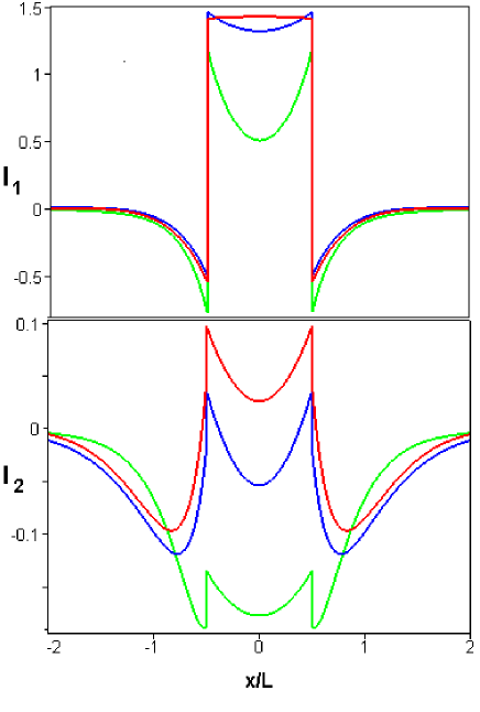
Figure 4: (Color online) Coordinate dependence of two phase shifted components of the spin-Hall current, as defined by Eqs. (37) and (41). $\Gamma_{so}/E_{Th}$=0.1 (red), 1 (blue),and 10 (green). The curves are calculated at $\pi k_{B}T/E_{Th}=0.5$ and $eV/E_{Th}=1$

.

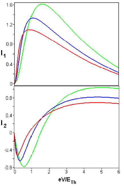
Figure 5: (Color online) Spin-Hall current as a function of the bias voltage at $\Gamma_{so}/E_{Th}=1$ and $x=0$. $\pi k_{B}T/E_{Th}$=0.25 (red), 0.5 (blue), and 1 (green).

A following important property of $J_{1},J_{2}$ and $J_{1\text{scr}},J_{2\text{scr}}$ calculated with functions and coefficients defined by Eqs. (27)-(36) takes place: all these partial contributions to the spin-Hall current, after initial increasing with the spin-orbit coupling $\alpha$, saturate when $\alpha\rightarrow\infty$. This behavior is already seen in $j_{0}(2\Omega,Q)$. Indeed, as follows from Eqs. (35) and (28), due to cancellation at $\Omega\rightarrow 0$ and $Q\rightarrow 0$ of two terms in brackets of (35) this function becomes constant at large $\Gamma_{so}\sim\alpha^{2}$. It can be checked that the same combination as in brackets of Eq.(35) enters into all terms contributing to the spin-Hall current. This sort of cancellation takes place also in normal systems and is inherent to all linear in $k$ SOI couplings. In normal systems it results in the vanishing stationary spin-Hall effect Engel . Indeed, there the spin current is driven by the stationary electric field which, due to charge screening, at the small screening length is homogeneous in samples of simple geometries. That guarantees $Q=0$ and, hence, the vanishing spin-Hall current. In contrast, in the considered here case of a nonstationary and inhomogeneous electron transport the spin-Hall current remains finite. The reason is that it is determined by the superconducting proximity effect, as it is discussed in the end of Section II. Consequently, a finite penetration range of Cooper pairs results in the finite $Q$. Moreover, there are also the ”surface” terms, like the $J_{2}$-term, localized near superconducting leads within the spin relaxation length $\sqrt{D/\Gamma_{so}}$. For these terms $DQ^{2}\sim\Gamma_{so}$. Therefore, they are not expected to saturate with larger SOI.

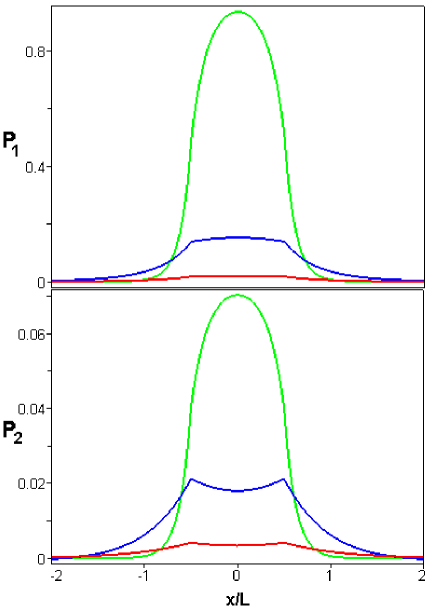
Figure 6: (Color online) Coordinate dependence of two phase shifted components of the spin polarization, as defined by Eqs. (39) and (42). $\Gamma_{so}/E_{Th}$=0.1 (red), 1 (blue),and 10 (green). The curves are calculated at $\pi k_{B}T/E_{Th}=0.5$ and $eV/E_{Th}=1$

.

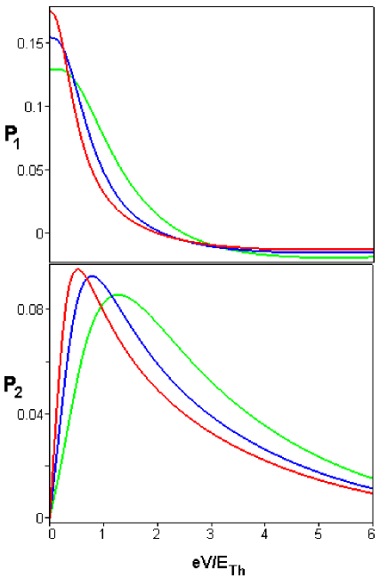
Figure 7: (Color online) Spin polarization as a function of the bias voltage at $\Gamma_{so}/E_{Th}=1$ and $x=0$. $\pi k_{B}T/E_{Th}$=1 (green), 0.5 (blue), and 0.1 (red).

We will normalize the spin-Hall current density according to

$$J_{s}=\frac{J_{c}}{e}\frac{m^{*}\alpha^{2}}{2\Gamma}I\,,$$ (37)

where $J_{c}$ is the critical Josephson current density defined by the sum over Matsubara frequencies $\omega=\pi k_{B}T(2n+1)$ as Aslamazov

$$J_{c}=\frac{e4\pi N_{F}k_{B}Ta^{2}}{\Gamma}\sum_{\omega\geqslant 0}\frac{|\Delta|^{2}}{|\Delta|^{2}+\omega^{2}}D_{00}(2i\omega,L)\,,$$ (38)

The diffuson in this equation is obtained as a Fourier transform from (28) and has the form $D_{00}(2i\omega,L)=\Gamma\exp(-\kappa L)/D\kappa$, with $\kappa=\sqrt{2\omega/D}$. The so defined dimensionless factor $I$ is of the order of 1. We note that although $\alpha$ can be quite large in narrow gap semiconductors Nitta , as well as in some metallic systems Ast , the parameter $m^{*}\alpha^{2}/\Gamma$ in Eq. 37 is small, because the diffusion approximation requires $k_{F}\alpha\ll\Gamma$.

The spin density is normalized as

$$S_{y}=S_{y0}P\,,$$ (39)

where $S_{y0}$ is the spin polarization induced by the critical Josephson current in the stationary case. This polarization is given by MalshukovSNS

$$S_{y0}=\frac{\alpha\tau}{2eD}J_{c}\,,$$ (40)

Since, according to (12), integrand in (II) contains terms proportional to $\delta_{\Omega,\pm eV}$, the normalized spin current and spin polarization can in general be represented as

$$I = -I_{1}\sin(2eVt)+I_{2}\cos(2eVt)$$ (41)

$$P = P_{1}\sin(2eVt)-P_{2}\cos(2eVt)\,.$$ (42)

The spatial distribution of $I_{1}$ and $I_{2}$ is shown in Fig. 4 at different values of the spin-orbit couplings. It is seen that the magnitude and direction of the spin-Hall current vary fast in the region of contacts. We recall in this connection that the contacts are assumed relatively narrow in Fig. 1 and are approximated by point-like sources placed at $x=\pm L/2$. At some moments of time the normalized spin current (42) changes its sign also as a function of $\Gamma_{so}$, as one can see from comparison of $I_{2}$ curves at $\Gamma_{so}=E_{Th}$ and $\Gamma_{so}=10E_{Th}$. Such changes are associated with discussed above cancellation of various contributions to the spin current at $eV$ and $k_{B}T\ll\Gamma_{so}$.

It have been pointed out that there are two types of terms, ”bulk” and ”surface” ones. At large $\Gamma_{so}$ the latter are localized near contacts, while the former penetrate deeper between and outside contacts. These qualitative features are clearly seen in Fig. 4. As expected, due to the spin-current saturation, the bulk contribution to the normalized current decreases with larger SOI. Indeed, $I_{1}$ is reduced in the middle of the junction at $\Gamma_{so}=10E_{Th}$ , while smaller changes are seen just near the contacts. At the same time, such a reduction is not so fast, as it was expected at first sight. At least, even at $\Gamma_{so}=10E_{Th}$ there is no considerable reduction of $I_{2}$ at $x=0$.

It is important to note that the spin current is not zero at $|x|>1/2$, while the Josephson current is absent there. In this region the former is driven by the time dependent potential, associated with the charge imbalance, rather than by a direct conversion of singlet Cooper pairs to triplet ones. In this spatial region the spin current is contributed by both ”surface” and ”bulk” terms. In Fig.4 it extends outside the junction over the range $\sim L$, because the both characteristic lengths $\sqrt{D/k_{B}T}$ and $\sqrt{D/eV}$ are taken of the order of $L$.

The voltage dependence of the spin-Hall current at $x=0$ and various temperatures is presented in Fig. 5. We note that both phase shifted components change sign at some voltages. At the same time, the behavior at the small bias is given by $I_{1}\sim V^{2}$ and $I_{2}\sim V$, as can also be checked analytically.

The coordinate dependence of the normalized spin polarization is shown in Fig. 6. In contrast to the considered previously stationary case MalshukovSNS , it is finite in the region $|x|>1/2$. Similar to the spin-Hall current, such a behavior can be explained by the charge imbalance effect. This effect becomes weaker at larger $\Gamma_{so}$. Indeed, at $\Gamma_{so}=10E_{Th}$ the magnitude of $P$ considerably increases inside the junction, while it becomes smaller outside it at $|x|>1/2$. This is opposite to the spin current trend observed in Fig.4. The reason is that the slow varying ”bulk” terms are not suppressed in $P$ at larger SOI, because in contrast to the spin current, there is no cancellation of the spin polarization at $DQ^{2}$ and $\Omega\ll\Gamma_{so}$.

A variation of the polarization with $V$ is presented in Fig. 7 for $\Gamma_{so}=E_{Th}$ . $P_{2}$ linearly turns to 0 at $V\rightarrow 0$, while $P_{1}$ reaches its maximum there. Our numerical results show also that the magnitude of $P_{1}$ at $V=0$ increases with $\Gamma_{so}\rightarrow\infty$, reaching 1, that can also be checked analytically. At the same time, the spatial dependence of $P_{1}$ takes the form of a step function, such that $P_{1}=1$ when $|x|<0.5L$ and $P_{1}=0$ at $|x|>0.5L$. Hence, as expected, in this limiting case the spin polarization coincides with polarization calculated in the regime of the stationary Josephson effect MalshukovSNS , after substitution in (42) of the phase factor $\sin(2eVt)$ by $\sin\phi$, where $\phi$ is the phase difference between superconductors.

In the considered here case the spin-Hall current carries the z-oriented time dependent spin polarization in the transverse (y) direction. Hence, the corresponding time dependent spin density can be accumulated at some distance near flanks of the junction, while in its bulk the y-polarization is finite between and outside contacts. The spin polarization might be detected by various methods employed in the case of the ordinary SHE Kato ; Valenzuela . Quite efficient is an all-electric method used in Ref. Valenzuela, . In this method a nonequilibrium spin polarization in the normal metal diffuses into an adjacent ferromagnet. On the other hand, it is well known Johnson , that the spin flux through a ferromagnet-normal metal interface induces a voltage difference across the interface, that can be measured. If we will try, however, to extend this method to the superconducting transport, we will face a problem of evaluating this voltage. It is well known how to calculate it in the case of a nonequilibrium flux of single particle spins. Much less, however, is known how to do this in our case, when triplet Cooper pairs contribute to this flux. Therefore, additional studies are necessary for a more complicated system than considered here.

This work has been supported by Taiwan NSC (Contract No. 96-2112-M-009-0038-MY3) and MOE-ATU grant.

Appendix A Derivation of basic equations

In this Abstract some explanations will be done of how Eqs. (II) and (18)-(II) have been derived within Keldysh diagrammatic technique. We start from definitions of Green functions entering into perturbation expansions. Each of the Green functions is the matrix in the Keldysh space Landau :

$$G=\left(\begin{array}[]{ccc}\hat{G}^{r}&\hat{G}^{K}\\ 0&\hat{G}^{a}\\ \end{array}\right)$$ (43)

The elements of this matrix are 2$\times$2 matrices in the Nambu space and 2$\times$2 matrices in the spin space. Besides, they depend on two time arguments and two wavevectors $\mathbf{k}$ and $\mathbf{k}^{\prime}$. These vectors are not equal, because there is no momentum conservation in the presence of impurity scattering. At the same time, the functions averaged over impurity positions become diagonal in the momentum space. Considering $G$ as matrices in $k$-space and also the tunneling amplitudes $t_{k,k^{\prime}}$ in Eq. (1) as elements of the matrix $\hat{t}$, one can write the expression for the spin current (4) in the fourth perturbation order with respect to the tunneling Hamiltonian (1) in the form

$$J_{s}(x,t)=\frac{1}{4}\int\prod_{i}dt_{i}\mathrm{Tr}[\sigma^{z}\langle\frac{\hat{k}}{m^{*}}\hat{G}_{11}(t-t_{1})\hat{t}\tilde{\hat{G}}_{12}(t_{1},t_{2})\hat{t}\hat{G}_{22}(t_{2}-t_{3})\hat{t}\tilde{\hat{G}}_{21}(t_{3},t_{4})\hat{t}\hat{G}_{11}(t_{4}-t)\rangle_{\text{imp}}]^{K}\,,$$ (44)

where $\tilde{\hat{G}}$ and $\hat{G}$ denote the Green function of the superconductor and the normal metal, respectively. The operator $\hat{k}=k_{y}\delta_{\mathbf{k},\mathbf{k}^{\prime}}$. We explicitly wrote the Nambu labels of functions, so that only the trace over spin and momentum variables must be taken in Eq. (44). Since only the Josephson tunneling is considered, in the perturbation expansion we take into account only anomalous $\tilde{\hat{G}}_{12}$ and $\tilde{\hat{G}}_{21}$ functions of superconducting leads, neglecting thus the usual stationary one-particle tunneling. These functions can be written in the form

$$\tilde{\hat{G}}_{12}(t,t^{\prime})=\hat{\cal{F}}(t-t^{\prime})\exp(\pm ieV(t+t^{\prime})/2)\,,$$ (45)

where the signs ”-” and ”+” relate to the left and right superconducting leads, respectively. $\tilde{\hat{G}}_{21}$ is obtained from this equation with the substitution $\cal{F}\rightarrow\cal{F}^{{\dagger}}$ and $V\rightarrow-V$. After Fourier transform of Green functions in Eq. (44), the time dependent exponential factors in $\tilde{\hat{G}}_{12}(t,t^{\prime})$ and $\tilde{\hat{G}}_{21}(t,t^{\prime})$ give the factors $\exp(\pm 2ieVt)$ in Eq. (II). It is important that the functions $\cal{F}$ and $\cal{F}^{{\dagger}}$ in Eq. (44) belong to different superconducting leads. Therefore, they are independently averaged over impurity positions and, hence, are diagonal in the momentum space. In the spin space they are proportional to the Pauli matrix $\sigma_{z}$, because, as it is discussed in Section II, these functions are associated with the singlet Cooper pairing.

It is easy to see that the Keldysh component of a product $ABCD...$ of matrices having the triangular form (43) can be written as the sum of products: $(A^{K}B^{a}C^{a}D^{a}...)+(A^{r}B^{K}C^{a}D^{a}...)+(A^{r}B^{r}C^{K}D^{a}...)+...$. In all these products the Keldysh function enters only once, while retarded and advanced functions are placed on the left and on the right from it, respectively. The time Fourier expansions of thermally equilibrium Keldysh functions $G$ and $\cal{F}$ can be expressed in terms of retarded and advanced functions as

$$\hat{G}^{K}(\omega)=\left(\hat{G}^{r}(\omega)-\hat{G}^{a}(\omega)\right)\tanh\frac{\omega}{2k_{B}T}\,.$$ (46)

We thus will apply the above expressions to the Keldysh component of the product in Eq.(44). This equation can be further simplified taking into account that $k_{B}T$, $eV\ll\Delta$ and distances of interest $\gg\sqrt{D/\Delta}$. Therefore, the main contribution to Eq.(44) is given by small frequencies $\omega\ll\Delta$. Since the difference of retarded and advanced anomalous functions $\cal{F}$ in Eq.(46) gives an expression proportional to $\delta\left(E^{2}_{k}+\Delta^{2}-\omega^{2}\right)$, the corresponding Keldysh component can be neglected for small $\omega$.

The next step is averaging over disorder. From Eqs. (44), (46), and taking into account that $\hat{\tilde{G}}\sim\sigma_{z}$ we get the following products to be averaged $\hat{G}^{r}_{11}\sigma_{z}\hat{G}^{r}_{22}\sigma_{z}\hat{G}^{r}_{11}$, $\hat{G}^{a}_{11}\sigma_{z}\hat{G}^{a}_{22}\sigma_{z}\hat{G}^{a}_{11}$, $\hat{G}^{r}_{11}\sigma_{z}\hat{G}^{a}_{22}\sigma_{z}\hat{G}^{a}_{11}$, and $\hat{G}^{r}_{11}\sigma_{z}\hat{G}^{r}_{22}\sigma_{z}\hat{G}^{a}_{11}$. In its turn, each of the Green functions is a sum of products $G_{k}U_{k,k_{1}}G_{k_{1}}U_{k_{1},k_{2}}...$, where $G_{k}$ are diagonal in $\mathbf{k}$ unperturbed functions and the number of impurity scattering amplitudes $U$ in each product is equal to the corresponding perturbation order. Calculation of such averages is described in many textbooks (for example, see Altshuler, ). Briefly, within the Born approximation, assuming random impurity positions the averages of $U_{k,k_{\prime}}$ products decouples into pair averages. In this way each pair enters as an effective two-particle interaction carrying a zero frequency. So, the average of a Green function can be expressed through the self-energy. In Eq. 6 this self-energy is given by $i\Gamma$. When a product of Green functions is averaged, a considerable simplification takes place in the semiclassical approximation when $\Gamma\ll E_{F}$. In this case a special class of the so called ”ladder” diagrams dominates in the perturbation expansion over disorder. Let us consider, for example the average $\langle\hat{G}^{r}_{11}\sigma_{z}\hat{G}^{r}_{22}\sigma_{z}\hat{G}^{r}_{11}\rangle_{\text{imp}}$. Combining in pairs $U$-s in $G^{r}_{22}$ with its neighbors on the left and on the right we obtain two ladder series. There are ”Cooperons”, according to definition (II). They are shown as gray boxes in Fig. 2a. At the same time, one can not build the ladder out of the pair $\hat{G}^{r}_{11}\bigotimes\hat{G}^{r}_{11}$. The reason is that the sum over $\mathbf{k}$ of a typical ladder element, the product $\hat{G}^{0r}_{\mathbf{k}11}\bigotimes\hat{G}^{0r}_{\mathbf{k}11}$, where $\hat{G}^{0r}$ is given by Eq. (6), turns to zero, because both functions have poles in the same semiplane of the complex variable $E_{k}$. On the same reason the ladders built of $\hat{G}^{r}_{22}\bigotimes\hat{G}^{a}_{11}$ also turn to zero, as follows from definition (6). Therefore, the average $\langle\hat{G}^{r}_{11}\sigma_{z}\hat{G}^{r}_{22}\sigma_{z}\hat{G}^{a}_{11}\rangle_{\text{imp}}$ contains only one Cooperon originating from the first two functions. Besides, the combination $\hat{G}^{r}_{11}\bigotimes\hat{G}^{a}_{11}$ entering into this product, results in a diffuson defined by Eq. (II). The corresponding Feynman diagram is shown in Fig. 2b.

In the same way, as the spin current, one may calculate the electric charge, substituting in Eq. (44) $\sigma^{z}k_{y}/2m^{*}$ for $e$. This charge is given by the sum of polygons in Figs. 3a and 3b. They represent $J_{1scr}$ and $J_{2scr}$, respectively. Further, the screening electric potential is calculated within the random phase approximation. This potential drives the spin-Hall effect in the same way as in normal systems. Engel

References

- (1) M. I. Dyakonov and V. I. Perel, Phys. Lett. A 35, 459 (1971); J. E. Hirsch, Phys. Rev. Lett. 83, 1834 (1999); S. Zhang, Phys. Rev. Lett. 85, 393(2000).
- (2) Y. K. Kato, R. C. Myers, A. C. Gossard, and D. D. Awschalom, Science 306, 1910 (2004)
- (3) J. Wunderlich, B. Kaestner, J. Sinova, and T. Jungwirth, Phys. Rev. Lett. 94, 047204 (2005)
- (4) S.O. Valenzuela and M. Tinkham, Nature 442, 176 (2006); E. Saitoh, M. Ueda, H. Miyajima, and G. Tatara, Appl. Phys. Lett 88, 182509 (2006); T. Seki, Yu Hasegawa, S. Mitani, S. Takahashi, H. Imamura, S. Maekawa, J. Nitta, K. Takanashi, Nature Mater. 7, 125 (2008); T. Kimura, Y. Otani, T. Sato, S. Takahashi, and S. Maekawa , Phys. Rev. Lett. 98, 156601 (2007).
- (5) H.-A. Engel, E. I. Rashba, and B. I. Halperin, in Handbook of Magnetism and Advanced Magnetic Materials, ed. by H. Kronmüller and S. Parkin (Wiley, Chichester, UK, 2007).
- (6) J. Makhlin, G. Schön, A. Shnirman, Rev. Mod. Phys. 73, 357 (2001)
- (7) D. I. Schuster et. al., Phys. Rev. Lett. 105, 140501 (2010); H. Wu, R. E. George, J. H. Wesenberg, K. Molmer, D. I. Schuster, R. J. Schoelkopf, K. M. Itoh, A. Ardavan, J. J. L. Morton, and G. A. D. Briggs, Phys. Rev. Lett. 105, 140503 (2010); Y. Kubo et. al., Phys. Rev. Lett. 105, 140502 (2010)
- (8) A. G. Mal’shukov and C. S. Chu, Phys. Rev. B 78, 104503 (2008)
- (9) L. P. Gor’kov and E. I. Rashba, Phys. Rev. Lett. 87, 037004 (2001)
- (10) H. Kontani, J. Goryo, and D. S. Hirashima, Phys. Rev. Lett. 102, 086602 (2009).
- (11) A. G. Mal’shukov, Severin Sadjina, and Arne Brataas Phys. Rev. B 81, 060502 (2010)
- (12) Yu. A. Bychkov and E. I. Rashba, J. Phys. C 17, 6039 (1984)
- (13) K. S. Tikhonov, Feigel’man, JETP Letters 89, 230 (2008); N. Argaman, Superlattices Microstruc. 25, 861 (1999)
- (14) E. M. Lifshitz and L. P. Pitaevskii, Physical Kinetics (Pergamon, New York, 1981).
- (15) V.M. Edelstein, Solid State Commun., 73, 233 (1990); F. T. Vas’ko and N. A. Prima, Sov. Phys. Solid State 21, 994 (1979); L. S. Levitov et al., Zh. Eksp. Teor. Fiz. 88, 229 (1985)[Sov. Phys. JETP 61, 133 (1985)]; A. G. Aronov and Yu. B. Lyanda-Geller, Pis’ma Zh. Eksp. Teor. Fiz. 50, 398 (1989) [JETP Lett. 50, 431 (1989)].
- (16) L. G. Aslamazov, A. I. Larkin, and Yu. N. Ovchinnikov, Zh. Eksp. Teor. Fiz. 55, 323 (1968),[Sov. Phys. JETP 28, 171 (1968)].
- (17) A.A. Abrikosov, L.P. Gor’kov, and I.E. Dzyaloshinskii, Methods of Quantum Field Theory in Statistical Physics, (Dover, New York, 1975)
- (18) B. L. Altshuler and A. G. Aronov, in Electron-Electron Interactions in Disordered Systems, edited by A. L. Efros and M. Pollak sNorth-Holland, Amsterdam, 1985.
- (19) M. Yu. Kupriyanov and V. F. Lukichev, Zh. Eksp. Teor. Fiz. 94, 139 (1988) [Sov. Phys. JETP 67, 1163 (1988).
- (20) E. G. Mishchenko, A. V. Shytov, and B. I. Halperin, Phys. Rev. Lett. 93, 226602 (2004); A. A. Burkov, A. S. Nunez, and A. H. MacDonald, Phys. Rev. B 70, 155308 (2004); A. G. Mal’shukov, L. Y. Wang, C. S. Chu and K. A. Chao, Phys. Rev.Lett. 95, 146601 (2005).
- (21) M. I. D’yakonov and V. I. Perel’, Sov. Phys. JETP 33, 1053 (1971) [Zh. Eksp. Teor. Fiz. 60, 1954 (1971)].
- (22) J. Nitta, T. Akazaki, and H. Takayanagi, Phys. Rev. Lett. 78, 1335 (1997) ; G. Engels, J. Lange, Th. Schäpers, and H. Lüth, Phys. Rev. B 55 , R1958 (1997); D. Grundler, Phys. Rev. Lett. 84, 6074 (2000).
- (23) C. R. Ast, J. Henk, A. Ernst, L. Moreschini, M. C. Falub, D. Pacile, P. Bruno, K. Kern, and M. Grioni, Phys. Rev. Lett. 98, 186807 (2007); I. Gierz, T. Suzuki, E. Frantzeskakis, S. Pons, S. Ostanin, A. Ernst, J. Henk, M. Grioni, K. Kern, C. R. Ast, Phys. Rev. Lett. 103, 046803 (2009)
- (24) M. Johnson and R. H. Silsbee, Phys. Rev. B 35, 4959 (1987); 37, 5312 (1988).