Strange nonchaotic attractors in quasiperiodically forced circle maps: Diophantine forcing

Abstract

We study parameter families of quasiperiodically forced (qpf) circle maps with Diophantine frequency. Under certain ${\cal C}^{1}$-open conditions concerning their geometry, we prove that these families exhibit nonuniformly hyperbolic behaviour, often referred to as the existence of strange nonchaotic attractors, on parameter sets of positive measure. This provides a nonlinear version of results by Young on quasiperiodic $\textrm{SL}(2,\mathbb{R})$-cocycles and complements previous results in this direction which hold for sets of frequencies of positive measure, but did not allow for an explicit characterisation of these frequencies. As an application, we study a qpf version of the Arnold circle map and show that the Arnold tongue corresponding to rotation number $1/2$ collapses on an open set of parameters.

The proof requires to perform a parameter exclusion with respect to some twist parameter and is based on the multiscale analysis of the dynamics on certain dynamically defined critical sets. A crucial ingredient is to obtain good control on the parameter-dependence of the critical sets. Apart from the presented results, we believe that this step will be important for obtaining further information on the behaviour of parameter families like the qpf Arnold circle map.

1 Introduction

After the discovery of strange chaotic attractors in two-dimensional dynamical systems like the Hénon map [1], a natural question that occurred was to determine the simplest type of smooth systems that exhibit ‘strange’ attractors. In particular, it was not clear whether chaos was a necessary prerequisite for the existence of such objects. Understanding ‘strange’ in a broad sense as ‘having a complicated structure and geometry’ (compare [2]), Grebogi et al gave a negative answer to this by showing that strange non-chaotic attractors (SNA) can appear in quasiperiodically forced (qpf) monotone interval maps [3]. Their argument was heuristic, but later made rigorous by Keller [4]. These findings prompted further investigations on qpf 1D maps, which have, despite their simple structure, surprisingly rich dynamics and appear as natural models for physical systems subject to the influence of two or more external periodic factors with incommensurate frequencies [5, 6, 7].

For quite a while, studies on the topic were mainly numerical and rigorous results remained rare. The only exception, apart from the very particular type of examples in [3, 4], is the rich theory of quasiperiodic (qp) $\textrm{SL}(2,\mathbb{R})$-cocycles and their associated linear-projective actions. For these systems, the existence of SNA had already been proved prior to the work of Grebogi et al by Millions̆c̆ikov [8], Vinograd [9] and, in a more general way, Herman [10]. In this context, the phenomenon is referred to as the non-uniform hyperbolicity of the cocycle. Due to close relations to the spectral properties of 1D Schrödinger operators with quasiperiodic potential (see, for example, [11, 12]), there have been intense efforts to understand the dynamics of qp $\textrm{SL}(2,\mathbb{R})$-cocycles during the last three decades (see [13, 14, 15, 16] for some recent advances). Unfortunately, most methods from this theory cannot simply be carried over to more general ‘non-linear’ qpf systems, since they strongly depend on the linear structure and, in many cases, on the close relations to spectral theory. At the same time, it is also difficult to compare SNA with the strange attractors appearing in Hénon-like maps, since on a formal level these are quite different objects. Nevertheless, the methods used by Benedicks and Carleson’s in their seminal work on the Hénon map [1] turned out to be equally fruitful for the description of SNA. Furthermore, the required inductive schemes are easier to implement in this context, such that one can reasonably hope to elaborate these techniques further in order to obtain additional insights about the behaviour and dynamics of parameter families of qpf circle maps. We will come back to this point at the end of the introduction.

In the context of qpf systems, multiscale analysis and parameter exclusion in the spirit of Benedicks and Carleson were introduced by Young in [17], where she described non-uniformly hyperbolic dynamics in certain parameter families of qp $\textrm{SL}(2,\mathbb{R})$-cocycles. The methods were then applied to qp Schrödinger cocycles by Bjerklöv [18], who also extended them to show the minimality of the dynamics. These results were so far restricted to linear-projective systems, but since the original setting in [1] is nonlinear it is not too surprising that it was eventually possible to adapt the techniques to qpf nonlinear models [19]. This allowed to prove the existence of SNA under rather general conditions. In [18, 19], the parameter exclusion was performed with respect to the forcing frequency. As a result, one obtains a set of frequencies of positive measure such that the considered system forced with these frequencies exhibits nonuniformly hyperbolic dynamics. The drawback is that this does not yield any statement about a fixed frequency like the golden mean, which is used in most of the numerical studies on the topic. Our aim here is to close this gap. This is achieved by performing a parameter exclusion with respect to some other suitable system parameter. We thus obtain a nonlinear version of the respective results in [17], augmented by the minimality of the dynamics. Using a particular symmetry, we further show that the Arnold tongue corresponding to rotation number $1/2$ collapses on an open set of parameters. While the collapse of tongues has already been described in [19], the robustness of this phenomenon seems to be new.

In order to state a qualitative version of our main result, we let ${\cal F}:=\{f\in\textrm{Diff}^{1}(\mathbb{T}^{2})\mid\pi_{1}\circ f=\pi_{1}\}$, where $\textrm{Diff}^{1}(\mathbb{T}^{2})$ denotes the group of diffeomorphisms of the two-torus $\mathbb{T}^{2}$ and $\pi_{1}$ is the projection to the first coordinate. Note that for $F\in{\cal F}$ we have $F(\theta,x)=(\theta,f_{\theta}(x))$ where $f_{\theta}(\cdot)=\pi_{2}\circ F(\theta,\cdot)$, such that we can view $F$ as a collection of fibre maps $(f_{\theta})_{\theta\in\mathbb{T}^{1}}$. Further, we let

$${\cal P}\ =\ \left\{(F_{\tau})_{\tau\in[0,1]}\mid F_{\tau}\in{\cal F}\ \forall\tau\in[0,1]\ \textrm{and}\ (\tau,\theta,x)\mapsto F_{\tau}(\theta,x)\textrm{ is }{\cal C}^{1}\right\}\$$

be the set of differentiable parameter families in ${\cal F}$. The fibre maps of $F_{\tau}$ are denoted by $f_{\tau,\theta}$, that is, $F_{\tau}(\theta,x)=(\theta,f_{\tau,\theta}(x))$. Finally, we let ${\cal D}(\sigma,\nu)$ be the set of frequencies $\omega\in\mathbb{T}^{1}$ that satisfy the Diophantine condition $d(n\omega,0)>\sigma\cdot|n|^{-\nu}\ \forall n\in\mathbb{Z}\setminus\{0\}$.

Theorem 1.1.

Given any constants $\sigma,\nu>0$, there exists a non-empty set ${\cal U}={\cal U}(\sigma,\nu)\subseteq{\cal P}$, open with respect to the induced ${\cal C}^{1}$-topology, with the following property:

For all $(F_{\tau})_{\tau\in[0,1]}\in{\cal U}$ and all $\omega\in{\cal D}(\sigma,\nu)$ there exists a set $\Lambda_{\infty}(\omega)\subseteq[0,1]$ of positive measure such that for all $\tau\in\Lambda_{\infty}(\omega)$ the qpf circle diffeomorphism

$$f_{\tau}\ :\ (\theta,x)\mapsto(\theta+\omega,f_{\tau,\theta}(x))$$

has a unique strange non-chaotic attractor (see Definition 2.1) which supports the unique physical measure of the system. Furthermore, the dynamics are minimal.

As in [19], we will provide two different quantitative versions of Theorem 1.1 which characterise the set ${\cal U}$ in terms of explicit ${\cal C}^{1}$-estimates. Since these conditions are somewhat technical, we postpone the precise statements to Section 3 and concentrate on two explicit examples.

The first quantitative result, Theorem 3.1 below, applies to the family

(1.1) $$f_{a,\tau}(\theta,x)\ =\ \left(\theta+\omega,\frac{1}{\pi}\arctan\left(a^{2}\tan(\pi x)\right)+g(\theta)+\tau\right)\$$

where $g:\mathbb{T}^{1}\to\mathbb{T}^{1}$ is a differentiable function that satisfies some non-degeneracy condition stated below. For example, one could take $g(\theta)=\sin(2\pi\theta)$. If we denote by $R_{\phi}$ the rotation matrix with angle $2\pi\phi$, then $f_{a,\tau}$ is the is the projective action of the qp $\textrm{SL}(2,\mathbb{R})$-cocycle given by

(1.2) $$A(\theta)\ =\ R_{g(\theta)+\tau}\cdot\left(\begin{array}[]{cc}a&0\\ 0&1/a\end{array}\right)\ .$$

For this particular system, we obtain the following statement.

Corollary 1.2 (to Theorem 3.1 below).

Suppose $g:\mathbb{T}^{1}\to\mathbb{T}^{1}$ is a differentiable function and there exists a finite set $\Omega_{0}$ such that for all $\tau\in\mathbb{T}^{1}\setminus\Omega_{0}$ the set $Z(\tau)=\{\theta\in\mathbb{T}^{1}\mid g(\theta)+\tau=\frac{1}{2}\}$ is finite and $g^{\prime}$ takes distinct and non-zero values at different points of $Z(\tau)$.

Then for all $\sigma,\nu>0$ there exists $a_{*}=a_{*}(g,\sigma,\nu)>0$ with the following property: for all $\omega\in{\cal D}(\sigma,\nu)$ and all $a\geq a_{*}$ there exists a set $\Lambda_{\infty}(a,\omega)\subseteq\mathbb{T}^{1}$ of positive measure such that for all $\tau\in\Lambda_{\infty}(a,\omega)$ the map $f_{a,\tau}$ given by (1.1) has a unique SNA and minimal dynamics. Further $\mathrm{Leb}_{\mathbb{T}^{1}}(\Lambda_{\infty}(a,\omega))$ goes to $1$ as $a\to\infty$.

The same result applies to any sufficiently small ${\cal C}^{1}$-perturbation of the parameter family (1.2).

This statement follows from Theorem 3.1 by some standard estimates. Since our main focus lies on the qpf Arnold circle map, we refer the reader to [19, Section 3.8] for details. We also note that the existence of an SNA for (1.1) is equivalent to the non-uniform hyperbolicity of the cocycle (1.2) [12, 20]. Hence, the result can be viewed as a perturbation-persistent version of [17, Theorem 2].

The second quantitative version of Theorem 1.1, stated as Theorem 3.2 below, is tailor-made for the application to the qpf Arnold circle map

(1.3) $$f_{a,b,\tau}(\theta,x)\ =\ \left(\theta+\omega,x+\tau+\frac{a}{2\pi}\sin(2\pi x)+g_{b}(\theta)\right)$$

with forcing function $g_{b}$ depending on some additional parameter $b$. The geometry of (1.3) is quite different to that of the previous example, since unlike in (1.1) the hyperbolicity on the single fibres is limited (the slope of the fibre maps $f_{a,b,\tau,\theta}$ remains bounded by $2$ in the invertible regime $|a|\leq 1$). In order to make up for this, the forcing function $g_{b}$ must have a particular shape that can be pushed to some extreme by adjusting the parameter $b$. General conditions for the family $g_{b}$ can be deduced from Theorem 3.2. (See also Remark 5.4.) Here, we concentrate again on an explicit example.

Corollary 1.3 (to Theorem 3.2 below).

Let

(1.4) $$g_{b}(\theta)\ =\ \arctan(b\sin(2\pi\theta))/\pi\qquad(b\in\mathbb{R})\ .$$

Then for all $\sigma,\nu>0$ and all $a>0$ there exists $b_{*}=b_{*}(\sigma,\nu,a)>0$ with the following property:

For all $\omega\in{\cal D}(\sigma,\nu)$ and all $b\geq b_{*}$ there exists a set $\Lambda_{\infty}(a,b,\omega)\subseteq\mathbb{T}^{1}$ of positive measure such that for all $\tau\in\Lambda_{\infty}(a,b,\omega)$ the map $f_{a,b,\tau}$ given by (1.3) has a unique SNA and minimal dynamics.

Apart from the restrictions on the forcing function coming from the lack of hyperbolicity, a further reason for the particular choice of $g_{b}$ in (1.4) is a special symmetry which appears at $\tau=\frac{1}{2}$. On the one hand, the lift $F$ of the map $f_{a,b,\frac{1}{2}}$ satisfies the relation

(1.5) $$F_{\theta}(-x)\ =\ 1-F_{\theta+1/2}(x)\ ,$$

and it can be easily seen that this forces the rotation number $\rho(f_{a,b,\frac{1}{2}})$ to be exactly $\frac{1}{2}$. On the other hand, the map $g_{b}+\frac{1}{2}$ takes values close to $\frac{1}{2}$ only on two intervals $I_{0}$ and $I_{0}+\frac{1}{2}$ around $0$ and $\frac{1}{2}$, respectively. These two intervals play a special role in the multiscale analysis, since they define the critical sets on the first level of the inductive scheme. Furthermore, as a consequence of (1.5) the fact that the $n$-th critical region consists of exactly two intervals $I_{n}$ and $I_{n}+\frac{1}{2}$ will remain true on all levels of the induction. This allows to control the return times of the critical regions directly by using only the Diophantine condition, and no parameters have to be excluded in order to avoid fast returns. In other words, in this particular situation the multiscale analysis can be performed without any parameter exclusion. As a consequence, we obtain the following.

Corollary 1.4 (to Theorem 3.2 below).

Suppose $g_{b}$ is chosen as in (1.4). Then for all $\sigma,\nu>0$ and $a>0$ there exists $b_{*}=b_{*}(\sigma,\nu,a)$ such that for all $\omega\in{\cal D}(\sigma,\nu)$ and $b>b_{*}$ the map $f_{a,b,\frac{1}{2}}$ has a unique SNA and minimal dynamics. $b_{*}(\sigma,\nu,\textbf{.})$ can be chosen constant on compact subsets of $(0,1)$.

This result has further consequences for the structure of the Arnold tongues

(1.6) $$A_{\rho}\ =\ \left\{(a,b,\tau)\in[0,1]\times\mathbb{R}\times[0,1]\mid\rho(f_{a,b,\tau})=\rho\right\}\$$

and the associated mode-locking plateaus

(1.7) $$P_{a,b,\rho}\ =\ \{\tau\in[0,1]\mid\rho(f_{a,b,\tau})=\rho\}\ ,$$

where $\rho(f_{a,b,\tau})$ denotes the fibred rotation number of $f_{a,b,\tau}$. We say a mode-locking plateau $P_{a,b,\rho}$ is collapsed if it consists of a single point. It is known that $P_{a,b,\rho}$ is collapsed for all $\rho\notin\mathbb{Q}+\mathbb{Q}\omega$ [21], and we implicitly assume that $\rho$ belongs to the module $\mathbb{Q}+\mathbb{Q}\omega$ whenever we speak of collapsed or non-collapsed plateaus. A tongue $A_{\rho}$ is said to be collapsed at $(a,b)$ if $P_{a,b,\rho}$ is collapsed. Minimal dynamics imply the collapse of a tongue, in the sense that whenever $f_{a,b,\tau}$ is minimal the tongue $A_{\rho}$ with $\rho=\rho(f_{a,b,\tau})$ is collapsed at $(a,b)$ (see Proposition 2.4). Hence, the tongue corresponding to rotation number $\frac{1}{2}$ is collapsed for all the parameters satisfying the assertions of Corollary 1.4.

Corollary 1.5.

Suppose $g_{b}$ is chosen as in (1.4). Then for all $\sigma,\nu>0$ there exists an open set $B(\sigma,\nu)\subseteq(0,1)\times\mathbb{R}^{+}$ such that for $\omega\in D(\sigma,\nu)$ and forcing function $g_{b}$ as in (1.4) the Arnold tongue $A_{\frac{1}{2}}$ is collapsed at all $(a,b)\in B(\sigma,\nu)$.

In [19], it was shown in a similar way that $A_{0}$ collapses on sets of parameters $(a,b)$ of positive measure, and the methods employed there would yield the same result for $A_{\frac{1}{2}}$. Hence, the new point here is the robustness of this phenomenon, that is, the openness of the set $B$ in Corollary 1.5.

As mentioned above, there are many further open problems concerning the behaviour of parameter families like (1.1) or (1.3). Probably the most prominent one is the question whether the rotation number as a function of the twist parameter is a ‘devils staircase’, meaning that the union of non-collapsed mode-locking plateaus is dense in the parameter interval. This is true for the unforced Arnold circle map. For qpf systems, existing results are again restricted to qp $\textrm{SL}(2,\mathbb{R})$-cocycles. A particular case is the projective action of the Schrödinger cocycle associated to the so-called almost-Mathieu operator, for which the question became known as the ‘Ten Martini Problem’. Recently it has been answered positively in full generality, meaning for all parameters and all irrational forcing frequencies, by Avila and Jitomirskaya [14] (after previous contributions by Béllisard and Simon [22] and Puig [13]). For the qpf Arnold circle map, still no rigorous results exist. Moreover the numerical findings are ambiguous. On the one hand, a devils staircase has been reported for some parameters regions in [6]. On the other hand the authors of [23] numerically detect parameters for which the 0-tongue is collapsed (a fact which is backed up by rigorous results in [19] and, replacing $0$ by $\frac{1}{2}$, also by Corollary 1.5) and report that for these parameters the mode-locking plateaus vanish and the rotation number strictly increases over a whole interval. In contrast to this, we believe that a further elaboration of the presented techniques should allow to prove the following.

Conjecture 1.6.

The set $\Lambda_{\infty}$ in Corollary 1.3 can be chosen such that it is contained in the closure of the union of non-collapsed mode-locking plateaus. The same is true for the parameter $\tau=\frac{1}{2}$ in the situation of Corollary 1.3.

In fact, what should be true is that all parameters $\tau$ for which the ‘slow-recurrence conditions’ $({\cal X^{\prime}})_{n}$ and $({\cal Y^{\prime}})_{n}$ introduced in the multiscale analysis scheme below are satisfied can be approximated by non-collapsed mode-locking plateaus. While this would not formally disprove the conjecture made in [23] (since our methods do not apply to the forcing function considered there), it would provide strong evidence for the fact that the observation is a numerical artifact. Furthermore, it could be a first step towards proving the existence of a devils staircase. Apart from the intrinsic interest of the above results, the hope to make further progress in this direction is one of the main motivations for the presented work.

Concerning the proofs, we will be able to rely to a great extent on the previous construction in [19]. In particular, the core part of the proof, which is the multiscale analysis for the dynamics of a fixed map under some non-recurrence conditions on certain dynamically defined critical sets, remains valid and can be used for our purpose without any modifications. We will therefore be able to concentrate almost exclusively on those aspects of the proof which differ from the previous one. The only drawback of this is that the present paper is not self-contained, but depends on a number of statements and estimates in [19]. However, as redoing all arguments would only result in an undue length of the paper and render the decisive differences in comparison to the previous construction less visible, this seems to be the appropriate way to proceed. In order not to leave the reader without any guidance, we will briefly motivate the used statements on a heuristic level.

Acknowledgements. I would like to thank Hakan Eliasson for inspiring discussions on the subject. This work was carried out in the Emmy-Noether-Group ’Low-dimensional and non-autonomous Dynamics’, which is supported by the Grant Ja 1721/2-1 of the German Research Council (DFG).

2 Notation and Preliminaries

2.1 Notation.

Given $a,b\in\mathbb{T}^{1}$, we denote by $[a,b]$ the positively oriented arc from $a$ to $b$. The same notation is used for open and half-open intervals. We write $b-a$ for the length of $[a,b]$, whereas the Euclidean distance between $a$ and $b$ will be denoted by $d(a,b)$. The derivative with respect to a variable $\xi$ will be denoted by $\partial_{\xi}$. On any product space, $\pi_{i}$ will denote the projection to the $i$-th coordinate. Quotient maps like the canonical projections $\mathbb{R}\to\mathbb{T}^{1}=\mathbb{R}/\mathbb{Z}$, $\mathbb{R}^{2}\to\mathbb{T}^{2}=\mathbb{R}^{2}/\mathbb{Z}^{2}$ or $\mathbb{T}^{1}\times\mathbb{R}\to\mathbb{T}^{2}$ will all be denoted by $\pi$.

If $I(\tau)=(a(\tau),b(\tau))$ is an interval that depends on some parameter $\tau\in\mathbb{R}$, then we say $I$ is differentiable in $\tau$ if this is true for both endpoints $a$ and $b$. In this case we write

$$|\partial_{\tau}I(\tau)|\ =\ \max\{|\partial_{\tau}a(\tau)|,|\partial_{\tau}b(\tau)|\}\ .$$

If $I^{\iota}(\tau)=(a^{\iota}(\tau),b^{\iota}(\tau))$ and $I^{\kappa}(\tau)=(a^{\kappa}(\tau),b^{\kappa}(\tau))$ are two disjoint intervals depending both on $\tau$, then we write

$$D_{\tau}(I^{\iota}(\tau),I^{\kappa}(\tau))\ >\ \eta$$

if there holds $\partial_{\tau}(y(\tau)-x(\tau))>\eta$ for all possible choices $x(\tau)=a^{\iota}(\tau),b^{\iota}(\tau)$ and $y(\tau)=a^{\kappa}(\tau),b^{\kappa}(\tau)$. We write

$$|D_{\tau}(I^{\iota}(\tau),I^{\kappa}(\tau))|\ >\ \eta$$

if either $D_{\tau}(I^{\iota}(\tau),I^{\kappa}(\tau))>\eta$ or $D_{\tau}(I^{\kappa}(\tau),I^{\iota}(\tau))>\eta$. In other words, $|D_{\tau}(I^{\iota}(\tau),I^{\kappa}(\tau))|>\eta$ means that the two intervals move with speed $>\eta$ relative to each other.

2.2 SNA in qpf systems.

We say a continuous map $f:\mathbb{T}^{2}\to\mathbb{T}^{2}$ is a qpf circle homeomorphism if it has skew product structure of the form

(2.1) $$f(\theta,x)\ =\ (\theta+\omega,f_{\theta}(x))$$

with irrational $\omega\in\mathbb{T}^{1}$. The maps $f_{\theta}(x)=\pi_{2}\circ f(\theta,x)$ are called fibre maps and we write $f^{n}_{\theta}(x)=\pi_{2}\circ f^{n}(\theta,x)$ for the fibre maps of the iterates. An invariant graph of $f$ is a measurable function $\varphi:\mathbb{T}^{1}\to\mathbb{T}^{1}$ that satisfies

(2.2) $$f_{\theta}(\varphi(\theta))\ =\ \varphi(\theta+\omega)\ .$$

The corresponding point set $\Phi=\{(\theta,\varphi(\theta))\mid\theta\in\mathbb{T}^{1}\}$ will equally be called an invariant graph. We note that in general multi-valued invariant graphs have to be taken into account as well. However, since in the situation we consider only single-valued invariant graphs occur, we restrict to this simple case. (The general definitions can be found in [19].)

To any invariant graph, an $f$-invariant ergodic measure $\mu_{\varphi}$ can be assigned by

(2.3) $$\mu_{\varphi}(A)\ =\ \mathrm{Leb}_{\mathbb{T}^{1}}\left(\pi_{1}(A\cap\Phi)\right)\ .$$

If all fibre maps are ${\cal C}^{1}$ and the derivative $f_{\theta}^{\prime}(x)$ is strictly positive and depends continuously on $(\theta,x)$, we speak of a qpf circle diffeomorphism. In this case, the (vertical) Lyapunov exponent of an invariant graph is defined as

(2.4) $$\lambda(\varphi)\ =\ \int_{\mathbb{T}^{1}}\log|\partial_{x}f_{\theta}(\varphi(\theta))|\ d\theta\ ,$$

In the particular context of qpf systems, SNA are now defined as follows.

Definition 2.1.

A non-continuous invariant graph with negative Lyapunov exponent is called a strange nonchaotic attractor (SNA). A non-continuous invariant graph with positive Lyapunov exponent is called a strange nonchaotic repeller (SNR).

Remark 2.2.

It should be said at this point that it it difficult to match this very specific definition of SNA with a general concept of strange attractors, as discussed for example in [2]. For instance, an attractor is usually understood to be a compact invariant set, but the point set associated to an SNA in the above sense is non-compact due to the non-continuity of the invariant graph. One could consider the closure of this set instead, but in the situations we describe this will be the whole two-torus, which cannot reasonably be called a ‘strange’ object. However, although the terminology might therefore be considered somewhat unfortunate, it has already been used for almost three decades in most of the vast physics literature on the topic. We therefore prefer to keep with it, simply taking it as a technical term specific to the theory qpf systems.

We also note that due to the negative Lyapunov exponent an SNA attracts a positive measure set of initial conditions and therefore carries a physical measure.

A convenient criterion for the existence of SNA involves pointwise Lyapunov exponents, forwards and backwards in time. These are given by

(2.5) $$\lambda^{\pm}(\theta,x)\ =\ \limsup_{n\to\infty}\frac{1}{n}|\log\partial_{x}f^{\pm n}_{\theta}(x)|\ .$$

The orbit of a point $(\theta,x)\in\mathbb{T}^{2}$ with $\lambda^{\pm}(\theta,x)>0$ is called a sink-source-orbit. The existence of such orbits implies the existence of SNA.

Proposition 2.3 ([19]).

Suppose $f$ is a quasiperiodically forced circle diffeomorphism which has a sink-source-orbit. Then $f$ has both a SNA and a SNR.

In the particular case of the Harper map, the existence of a sink-source-orbit is equivalent to Anderson localisation for the corresponding almost-Mathieu operator (see, for example, [12] or [20, Section 1.3]).

2.3 The fibred rotation number and mode-locking.

If a qpf circle homeomorphism $f$ is homotopic to the identity on $\mathbb{T}^{2}$, it has a continuous lift $F:\mathbb{T}^{1}\times\mathbb{R}\to\mathbb{T}^{1}\times\mathbb{R}$ of the form $F(\theta,x)=(\theta+\omega,F_{\theta}(x))$. In this case, the limit

(2.6) $$\rho(F)=\lim_{n\rightarrow\infty}(F^{n}_{\theta}(x)-x)/n$$

exists and is independent of $(\theta,x)$ [10, Section 5.3]. $\rho(f):=\rho(F)\bmod 1$ is called the (fibred) rotation number of $f$. If the rotation number remains constant under all sufficiently small ${\cal C}^{0}$-perturbations, we speak of mode-locking. The mechanism for mode-locking has been clarified in [21]. For our purposes we need the following two consequences.

Proposition 2.4 ([21, 19]).

Suppose $f$ is a qpf circle homeomorphism and let $f_{\epsilon}=R_{\epsilon}\circ f$, where $R_{\epsilon}(\theta,x)=(\theta,x+\epsilon)$. Then the following holds.

• If $\rho(f)\notin\mathbb{Q}+\mathbb{Q}\omega$ then $\epsilon\mapsto\rho(f_{\epsilon})$ is strictly increasing in $\epsilon=0$.

• If $f$ is minimal then $\epsilon\mapsto\rho(f_{\epsilon})$ is strictly increasing in $\epsilon=0$.

In other words, mode-locking cannot occur in situations (a) and (b).

3 Statement of the main results

The explicit ${\cal C}^{1}$-open conditions characterising the set ${\cal U}$ in Theorem 1.1 are not too complicated if each one is considered by itself, but altogether they form a rather long list. We therefore prefer not to include them in Theorem 3.1, but to state them separately before. We also note that conditions (${\cal A}1$)–(${\cal A}6$) below are precisely those used in [19], whereas the Diophantine condition (${\cal A}0$) and the assumptions (${\cal A}8$)–(${\cal A}10$) on the dependence on the twist parameter are new. Let $\Lambda\subseteq[0,1]$ be an open interval.

I. Diophantine condition. First, recall that $\omega\in{\cal D}(\sigma,\nu)$ just means that

($${\cal A}0 d(n\omega,0)\ >\ \sigma\cdot|n|^{-\nu}\quad\forall n\in\mathbb{Z}\setminus\{0\}\ .$$)

II. Critical regions. Let $E=[e^{-},e^{+}]$ and $C=[c^{-},c^{+}]$ be two non-empty, compact and disjoint subintervals of $\mathbb{T}^{1}$. We will assume that for all $\tau\in\Lambda$ there exists a finite union ${\cal I}_{0}(\tau)\subseteq\mathbb{T}^{1}$ of ${\cal N}$ disjoint open intervals $I_{0}^{1}(\tau),\ldots,I_{0}^{\cal N}(\tau)$ (the ‘critical regions’) such that

($${\cal A}1 f_{\tau,\theta}(\mbox{cl}(\mathbb{T}^{1}\setminus E))\ \subseteq\ \mbox{int}(C)\ \ \ \ \ \forall\theta\notin{\cal I}_{0}(\tau)\ .$$)

Note that this implies

($${\cal A}1^{\prime} f_{\tau,\theta}^{-1}(\mbox{cl}(\mathbb{T}^{1}\setminus C))\ \subseteq\ \mbox{int}(E)\ \ \ \ \ \forall\theta\notin{\cal I}_{0}(\tau)+\omega\ .$$)

III. Bounds on the derivatives. Concerning the derivatives of the fibre maps $f_{\tau,\theta}$, we will assume that for given $\alpha>1$ and $p\in\mathbb{N}$ we have

($${\cal A}2 \alpha^{-p}\ <\ \partial_{x}f_{\tau,\theta}(x)\ <\ \alpha^{p}\hskip 20.00003pt\quad\forall(\theta,x)\in\mathbb{T}^{2}\ ;$$)

($${\cal A}3 \hskip 30.00005pt\partial_{x}f_{\tau,\theta}(x)\ >\ \alpha^{2/p}\hskip 41.00012pt\quad\forall(\theta,x)\in\mathbb{T}^{1}\times E\ ;$$)

($${\cal A}4 \hskip 30.00005pt\partial_{x}f_{\tau,\theta}(x)\ <\ \alpha^{-2/p}\hskip 41.00012pt\quad\forall(\theta,x)\in\mathbb{T}^{1}\times C\ .$$)

Further, we fix $S>0$ such that

($${\cal A}5 |\partial_{\theta}f_{\tau,\theta}(x)|\ <\ S\ \ \ \ \ \forall(\theta,x)\in\mathbb{T}^{2}\ .$$)

IV. Transversal Intersections. The significance of the critical region ${\cal I}_{0}(\tau)$ is the fact that due to (${\cal A}1$) this is the only place where the attracting and the repelling region can ‘mix up’. In order to ensure that the intersections of $f_{\tau}({\cal I}_{0}(\tau)\times C)$ and $({\cal I}_{0}(\tau)+\omega)\times E$ are ‘nice’ (transversal in an appropriate sense), we will assume that

($${\cal A}6 \begin{array}[]{l}\exists!\theta_{\iota}^{1}\in I_{0}^{\iota}(\tau)\textrm{ with }f_{\tau,\theta_{\iota}^{1}}(c^{+})=e^{-}\textrm{ \ and }\\ \exists!\theta_{\iota}^{2}\in I_{0}^{\iota}(\tau)\textrm{ with }f_{\tau,\theta_{\iota}^{2}}(c^{-})=e^{+}\ .\end{array}$$)

This ensures that the image of $I_{0}^{\iota}(\tau)\times C$ crosses the strip $(I^{\iota}_{0}(\tau)+\omega)\times E$ exactly once and not several times. In order to control the slope of these strips, we will assume that

($${\cal A}7 |\partial_{\theta}f_{\tau,\theta}(x)|\ >\ s\ \ \ \ \ \forall(\theta,x)\in{\cal I}_{0}(\tau)\times\mathbb{T}^{1}\$$)

for some constant $s$ with $0<s<S$.

V. Dependence on $\tau$. First, we fix an upper bound $L$ on $|\partial_{\tau}f_{\tau,\theta}(x)|$, that is,

($${\cal A}8 |\partial_{\tau}f_{\tau,\theta}(x)|\ <\ L\ \ \ \ \ \forall(\theta,x)\in\mathbb{T}^{2}\ .$$)

Secondly, we assume that all connected components $I^{\iota}_{0}(\tau)=(a^{\iota}_{0}(\tau),b^{\iota}_{0}(\tau))$ of ${\cal I}_{0}(\tau)$ are differentiable with respect to $\tau$ and that for some constant $\eta>0$ we have

($${\cal A}9 |D_{\tau}(I^{\iota}_{0}(\tau),I^{\kappa}_{0}(\tau))|\ >\ \eta/2\quad\forall\iota\neq\kappa\in[1,\cal N]\ .$$)

Finally we will need an assumption which ensures that condition (${\cal A}9$) holds in a similar way for the higher order critical regions ${\cal I}^{\iota}_{n}$ defined later on. This is actually the crucial point of the construction, which allows to adapt the parameter exclusion scheme from [18, 19] to the considered problem. For any $\iota\in[1,{\cal N}]$ we let

$$Q^{\iota}(\tau)\ :=\ \left\{\partial_{\tau}f_{\tau,\theta}(x)/\partial_{\theta}f_{\tau,\theta}(x)\left|\ (\theta,x)\in I^{\iota}_{0}\times\mathbb{T}^{1}\right.\right\}\ .$$

Then we assume that there holds

($${\cal A}10 d(Q^{\iota}(\tau),Q^{\kappa}(\tau))\ >\ \eta\quad\forall\iota\neq\kappa\in[1,\cal N]\ .$$)

Theorem 3.1.

Let $\omega\in{\cal D}(\sigma,\nu)$ and $\delta>0$. Suppose that $\Lambda\subseteq[0,1]$ is an open interval and $(F_{\tau})_{\tau\in[0,1]}\in{\cal P}$ is such that conditions (${\cal A}1$)–(${\cal A}10$) are satisfied on $\Lambda$. Let $\epsilon_{0}:=\sup_{\iota\in[1,{\cal N}],\tau\in\Lambda}|I^{\iota}_{0}(\tau)|$. Then there exist constants $\alpha_{*}=\alpha_{*}(\sigma,\nu,{\cal N},p,S,s,L,\eta,\delta)$ and $\epsilon_{*}=\epsilon_{*}(\sigma,\nu,{\cal N},p,S,s,L,\eta,\delta)$ such that the following holds.

If $\alpha>\alpha_{*}$ and $\epsilon_{0}<\epsilon_{*}$, then there exists a set $\Lambda_{\infty}=\Lambda_{\infty}(\omega)\subseteq\Lambda$ of measure $\mathrm{Leb}(\Lambda_{\infty})>\mathrm{Leb}(\Lambda)-\delta$ such that for all $\tau\in\Lambda_{\infty}$ the qpf circle diffeomorphism

(3.1) $$f_{\tau}\ :\ (\theta,x)\mapsto(\theta+\omega,f_{\tau,\theta}(x))$$

satisfies

$$(*) \left\{\begin{array}[]{cl}(*1)&f_{\tau}\textrm{ has a SNA }\varphi^{-}\textrm{ and a SNR }\varphi^{+};\vspace{1ex}\\ \vspace{1ex}(*2)&\varphi^{-}\textrm{ and }\varphi^{+}\textrm{ are one-valued and the only invariant graphs of }f;\\ (*3)&f_{\tau}\textrm{ is minimal.}\end{array}\right.$$

Further, if $f_{\tau_{0}}$ satisfies

(3.2) $$f_{\tau_{0},\theta+\frac{1}{2}}(-x)\ =\ -f_{\tau_{0},\theta}(x)\qquad\forall(\theta,x)\in\mathbb{T}^{2}$$

then $\tau_{0}\in\Lambda_{\infty}$.

The proof is given in Section 4.

VI. Modified assumptions. As mentioned in the introduction, it is not possible to apply this result to the qpf Arnold circle map due to the bounded slope of the fibre maps. In order to make up for this lack of hyperbolicity, a particular geometry and symmetry of the forcing has to be used. For the twist parameter exclusion carried out here, this is slightly more subtle than for the frequency exclusion in [19] and stronger conditions on the forcing are required (see also Remark 5.4). First, we have to restrict to the case of two critical regions with fixed distance $1/2$.

($${\cal A}7^{\prime} \textstyle{\cal N}=2\ \textrm{ and there holds }\ I^{1}_{0}(\tau)=I^{2}_{0}(\tau)+\frac{1}{2}\ .$$)

Secondly, the slope on the two critical regions must have opposite sign.

($${\cal A}8^{\prime} \partial_{\theta}f_{\tau,\theta}(x)>s\ \textrm{ on }\ I^{1}_{0}\times\mathbb{T}^{1}\ \textrm{ and }\partial_{\theta}f_{\tau,\theta}(x)<-s\ \textrm{ on }I^{2}_{0}\times\mathbb{T}^{1}\ .$$)

Thirdly, as in [19] we need to ensure that away from the critical regions the $\theta$-dependence is small. To that end, we suppose ${\cal I}_{0}^{\prime}\subseteq\mathbb{T}^{1}$ is the disjoint union of two open intervals $I^{1^{\prime}}_{0}$ and $I^{2^{\prime}}_{0}=I^{1^{\prime}}_{0}+\frac{1}{2}$ with $I^{k}_{0}\subseteq I^{k^{\prime}}_{0}$ $(k=1,2)$ and for some $s^{\prime}\in(0,s)$ there holds

($${\cal A}9^{\prime} |\partial_{\theta}f_{\theta}(x)|\ <\ s^{\prime}\ \ \forall(\theta,x)\in(\mathbb{T}^{1}\setminus{\cal I}_{0}^{\prime})\times C\ .$$)

Finally, we need constants $\gamma,L>0$ which provide uniform upper and lower bounds for the dependence on the twist parameter $\tau$.

($${\cal A}10^{\prime} \gamma\ <\ \partial_{\tau}f_{\tau,\theta}(x)\ <\ L\qquad$$)

Theorem 3.2.

Let $\omega\in{\cal D}(\sigma,\nu)$ and $\delta>0$. Suppose that $\Lambda\subseteq[0,1]$ is an open interval and $(F_{\tau})_{\Lambda\in[0,1]}\in{\cal P}$ is such that conditions (${\cal A}0$)–(${\cal A}6$) and (${\cal A}7^{\prime}$)–(${\cal A}10^{\prime}$) are satisfied on $\Lambda$. Let $\epsilon_{0}:=\sup_{\iota\in[1,{\cal N}],\tau\in\Lambda}|I^{\iota}_{0}(\tau)|$. Further, assume there exist constants $A,d>1$ such that

(3.3) $$S < A\cdot d\ ,$$

(3.4) $$s > d/A\ ,$$

(3.5) $$\epsilon_{0} < A/\sqrt{d}\ ,$$

(3.6) $$s^{\prime} < A\ .$$

Then there exist a constant $d_{*}=d_{*}(\sigma,\nu,{\cal N},\alpha,p,L,\gamma,A,\delta)>0$ with the following property.

If $d>d_{*}$, then there exists a set $\Lambda_{\infty}=\Lambda_{\infty}(\omega)\subseteq\Lambda$ of measure $\mathrm{Leb}(\Lambda_{\infty})>\mathrm{Leb}(\Lambda)-\delta$ such that for all $\tau\in\Lambda_{\infty}$ the qpf circle diffeomorphism

(3.7) $$f_{\tau}\ :\ (\theta,x)\mapsto(\theta+\omega,f_{\tau,\theta}(x))$$

satisfies $(*)$ ‣ 3.1. Further, if $f_{\tau_{0}}$ satisfies (3.2) then $\tau_{0}\in\Lambda_{\infty}$.

The proof is given in Section 5. We note that the precise form of the $d$-dependence in (3.3)–(3.6) is to some extent arbitrary and could be stated in a more general way, but we refrain from introducing even more parameters and refer to Section 5.2 for details. The estimates required to deduce Corollaries 1.3–1.5 from this statement will be carried out in Section 5.3.

4 The basic version of the twist parameter exclusion

4.1 Critical sets and critical regions.

In this section, we will briefly recall the construction from [19] and collect the key statements needed for the proof of Theorem 3.1. The parameter $\tau$, and consequently the map $f_{\tau}$, will be fixed. Nevertheless we keep the dependence on $\tau$ explicit for the sake of consistency with the later sections. The description of the dynamics of a suitable qpf circle diffeomorphism $f$ in [19] is based on the analysis of certain critical sets ${\cal C}_{0},{\cal C}_{1},{\cal C}_{2},\ldots$ and critical regions ${\cal I}_{0},{\cal I}_{1},{\cal I}_{2},\ldots$, which are given as follows.

Given a union ${\cal I}_{0}(\tau)$ of ${\cal N}$ disjoint open intervals $I^{1}_{0}(\tau)\ldots I^{\cal N}_{0}(\tau)$ and a monotonically increasing sequence of integers $(M_{n})_{n\in\mathbb{N}_{0}}$ with $M_{0}\geq 2$, we recursively define

$${\cal A}_{n} := \{(\theta,x)\mid\theta\in{\cal I}_{n}(\tau)-(M_{n}-1)\omega,\ x\in C\}\ ,$$

$${\cal B}_{n} := \{(\theta,x)\mid\theta\in{\cal I}_{n}(\tau)+(M_{n}+1)\omega,\ x\in E\}\ ,$$

$${\cal C}_{n} := f_{\tau}^{M_{n}-1}({\cal A}_{n})\cap f^{-M_{n}-1}({\cal B}_{n})\quad\textrm{and }$$

$${\cal I}_{n+1}(\tau) := \mathrm{int}(\pi_{1}({\cal C}_{n}))\ .$$

The crucial observation is the fact that certain ‘slow recurrence’ assumptions on the critical regions ${\cal I}_{n}$ are already sufficient to guarantee the nonuniform hyperbolicity of $f_{\tau}$. In order to state them, suppose $(K_{n})_{n\in\mathbb{N}_{0}}$ is a monotonically increasing sequence of positive integers and $(\epsilon_{n})_{n\in\mathbb{N}_{0}}$ is a non-increasing sequence of positive real numbers which satisfy $\epsilon_{0}\leq 1$ and $\epsilon_{n}\geq 9\epsilon_{n+1}\ \forall n\in\mathbb{N}_{0}$. Let

$${\cal X}_{n}\ :=\ \bigcup_{k=1}^{2K_{n}M_{n}}({\cal I}_{n}+k\omega)\ \ \textrm{ and }\ \ {\cal Y}_{n}\ :=\ \bigcup_{j=0}^{n}\bigcup_{k=-M_{j}+1}^{M_{j}+1}({\cal I}_{j}+k\omega)\ .$$

Then the required assumptions on the critical regions are the following.

$$({\cal X})_{n} d({\cal I}_{j},{\cal X}_{j})\ >\ 3\epsilon_{j}\ \ \ \ \ \forall j=0,\ldots,n\ ,$$

$$({\cal Y})_{n} d(({\cal I}_{j}-(M_{j}-1)\omega)\cup({\cal I}_{j}+(M_{j}+1)\omega),{\cal Y}_{j-1})\ >\ 0\ \ \ \ \ \forall j=1,\ldots,n\ .$$

Let $\beta_{0}=1$, $\beta_{n}=\prod_{j=0}^{n-1}\left(1-\frac{1}{K_{j}}\right)$ and $\beta=\lim_{n\rightarrow\infty}\beta_{n}$. Further, define

(4.1) $$\alpha_{\infty}\ =\ \alpha^{2\beta/p-(1-\beta)p}\ .$$

Proposition 4.1 (Propositions 3.10 in [19]).

If (${\cal A}1$)–(${\cal A}7$) hold, $\alpha_{\infty}>\alpha_{1}$ and for all $n\in\mathbb{N}_{0}$ conditions $({\cal X})_{n}$ and $({\cal Y})_{n}$ are satisfied and ${\cal I}_{n+1}(\tau)=\pi_{1}({\cal C}_{n})\neq\emptyset$, then $f_{\tau}$ has a sink-source orbit and consequently an SNA and an SNR.

We will also use the following slightly stronger versions of the above conditions.

$$({\cal X^{\prime}})_{n} d({\cal I}_{j},{\cal X}_{j})\ >\ 9\epsilon_{j}\ \ \ \ \ \forall j=0,\ldots,n\ ,$$

$$({\cal Y^{\prime}})_{n} d(({\cal I}_{j}-(M_{j}-1)\omega)\cup({\cal I}_{j}+(M_{j}+1)\omega),{\cal Y}_{j-1})\ >\ 2\epsilon_{j}\ \ \ \ \ \forall j=1,\ldots,n\ .$$

Remark 4.2.

In the proof of Theorems 3.1 and 3.2, we will show that for all $\tau\in\Lambda_{\infty}$ conditions $({\cal X^{\prime}})_{n}$ and $({\cal Y^{\prime}})_{n}$ hold. In fact, for our purposes here the weaker conditions $({\cal X})_{n}$ and $({\cal Y})_{n}$ would be sufficient, since we only need them for the application of Proposition 4.1. The reason for using the stronger versions $({\cal X^{\prime}})_{n}$ and $({\cal Y^{\prime}})_{n}$ is that we believe these to be crucial in a current approach to the proof of Conjecture 1.6, and that at the same time this inflicts no extra costs whatsoever.

Let us briefly review the construction in [19] that leads to the statement of Proposition 4.1 and provide some more details that will be used later. Given any point $(\theta_{0},x_{0})\in\mathbb{T}^{2}$, we denote its iterates by $(\theta_{k},x_{k})=f_{\tau}^{k}(\theta_{0},x_{0}),\ k\in\mathbb{Z}$. Now, (${\cal A}1$) implies that whenever $\theta_{0}\notin{\cal I}_{0}(\tau)$ and $x_{0}\in C$, the forward orbit remains ‘trapped’ in the contracting region $\mathbb{T}^{1}\times C$ until $\theta_{k}$ enters ${\cal I}_{0}(\tau)$ for the first time. However, even if $\theta_{k}\in{\cal I}_{0}(\tau)$ and the orbit enters the expanding region at time $k$, that is $x_{k+1}\in E$, it will leave $\mathbb{T}^{1}\times E$ again after $M_{0}$ further iterates unless $\theta_{k}$ is also contained in the smaller set ${\cal I}_{1}(\tau)$. (This is a straightforward consequence of the definition of ${\cal C}_{0}$ and ${\cal I}_{1}(\tau)$.) Following this idea it is possible, via a purely combinatorial inductive construction, to control the behaviour of an orbit $(\theta_{k},x_{k})$ starting in ${\cal A}_{n}$ up to the first time $\hat{k}\in\mathbb{N}$ at which $\theta_{k}$ enters the $(n+1)$-th critical region ${\cal I}_{n+1}(\tau)$, provided that the ‘slow recurrence’ assumptions $({\cal X})_{n}$ and $({\cal Y})_{n}$ hold [19, Lemma 3.4]. In this case, the finite trajectory will remain in $\mathbb{T}^{1}\times C$ most of the time and the fraction of time spent outside this set is at most $1-\beta_{n}$ [19, Lemma 3.8].

As a consequence, since $M_{n}\leq\hat{k}$ by $({\cal X})_{n}$, it is possible to control the forward orbit of these points up to time $M_{n}$, or equivalently the backward orbit of points in $f_{\tau}^{M_{n}}({\cal A}_{n})\supseteq{\cal C}_{n}$, which remain trapped in the contracting region most of the time. Similar findings hold for the forwards orbits of points in $f^{-M_{n}}_{\tau}({\cal B}_{n})\supseteq{\cal C}_{n}$, which remain in the expanding region most of the time. Combining the combinatorial information about the behaviour of the orbits with the estimates on the derivatives provided by (${\cal A}2$)–(${\cal A}4$) one obtains the following statement.

Lemma 4.3 (Corollaries 3.7 and 3.9 in [19]).

Suppose (${\cal A}1$)–(${\cal A}4$), $({\cal X})_{n}$ and $({\cal Y})_{n}$ hold and $(\theta,x)\in\mathrm{cl}(f_{\tau}({\cal C}_{n}))$. Then for all $k\in[0,M_{n}]$ we have

(4.2) $$\partial_{x}f_{\tau,\theta}^{-k}(x)\geq\alpha_{\infty}^{k}\quad\textrm{and}\quad\partial f_{\tau,\theta}^{k}(x)\geq\alpha_{\infty}^{k}\ .$$

Furthermore, there holds ${\cal C}_{0}\supseteq{\cal C}_{1}\supseteq\ldots\supseteq{\cal C}_{n+1}$ and

(4.3) $$(\theta,x)\in({\cal I}_{n}(\tau)+\omega)\times E\quad,\quad f_{\tau}^{-1}(\theta,x)\in{\cal I}_{n}(\tau)\times C\ .$$

This statement rather easily entails Proposition 4.1 (respectively [19, Proposition 3.10]): When $({\cal X})_{n}$ and $({\cal Y})_{n}$ hold for all $n\in\mathbb{N}$ and $(\theta,x)\in\bigcap_{n\in\mathbb{N}}\mathrm{cl}\left(f_{\tau}({\cal C}_{n})\right)$, then it follows directly from (4.2) that the point $(\theta,x)$ has a positive vertical Lyapunov exponent both for $f_{\tau}$ and for its inverse $f^{-1}_{\tau}$. Hence, there exist a sink-source-orbit and thus an SNA by Proposition 2.3.

Due to Proposition 4.1, the validity of the slow recurrence conditions $({\cal X})_{n}$ and $({\cal Y})_{n}$ together with ${\cal I}_{n}(\tau)\neq\emptyset$ provides a rigorous criterion for the existence of SNA. The remaining task is to find a positive measure set of parameters (frequencies $\omega$ in [19], parameters $\tau$ in our setting) for which these assumptions are satisfied for all $n\in\mathbb{N}$. At this point, a detailed analysis of the geometry of the critical sets, or more precisely of the sets $f^{M_{n}}_{\tau}({\cal A}_{n})$ and $f^{-M_{n}}_{\tau}({\cal B}_{n})$ whose intersection equals $f_{\tau}({\cal C}_{n})$, comes into play. The outcome is that the size of the connected components of the critical regions ${\cal I}_{n}(\tau)$ decays super-exponentially with $n$ and that these components depend ‘nicely’ on the parameter. This will be made precise in Proposition 4.3 and Lemma 4.5 below.

The main idea behind this geometric analysis is again the fact that for any connected component $I^{\iota}_{n}(\tau)$ of ${\cal I}_{n}(\tau)$ the first $M_{n}-1$ forward iterates of the set $A^{\iota}_{n}=(I^{\iota}_{n}(\tau)-(M_{n}-1)\omega)\times C$ remain in the contracting region most of the time. Consequently $f_{\tau}^{M_{n}-1}(A^{\iota}_{n})$ will be a very thin strip, which will moreover be almost horizontal since the strong contraction ‘kills’ any dependence on $\theta$. Due to (${\cal A}7$) the image $f_{\tau}^{M_{n}}(A^{\iota}_{n})$ will then have slope $\geq s/2$. It therefore intersects the image $f_{\tau}^{-M_{n}}(B^{\iota}_{n})$ of $B^{\iota}_{n}=(I^{\iota}_{n}(\tau)+(M_{n}+1)\omega)\times E$ in a transversal way, since this set is a very thin horizontal strip by the same reasoning as for $f_{\tau}^{M_{n}-1}(A^{\iota}_{n})$. (Note that the expanding region $\mathbb{T}^{1}\times E$ is contracted by the inverse $f^{-1}$.) Consequently the resulting intersection $f_{\tau}^{M_{n}}(A^{\iota}_{n})\cap f_{\tau}^{-M_{n}}(B^{\iota}_{n})$ always has the geometry depicted in Figure 4.1 and projects to a very small interval $I^{\iota}_{n+1}(\tau)+\omega$.

In order to give a more detailed quantitative version of this heuristic description, we first define the ‘bounding graphs’ of the sets $f_{\tau}^{M_{n}}(A^{\iota}_{n})$ and $f_{\tau}^{-M_{n}}(B^{\iota}_{n})$. For $\theta\in I^{\iota}_{n}(\tau)+\omega$, let

(4.4) $$\varphi_{\iota,n}^{\pm}(\theta,\tau)\ :=\ f_{\tau,\theta-M_{n}\omega}^{M_{n}}(c^{\pm})\quad\textrm{ and }\quad\psi_{\iota,n}^{\pm}(\theta,\tau)\ :=\ f_{\tau,\theta+M_{n}\omega}^{-M_{n}}(e^{\pm})\ .$$

Note that we have

(4.5) $$f_{\tau}^{M_{n}}(A^{\iota}_{n}) = \{(\theta,x)\mid\theta\in I_{n}^{\iota}(\tau)+\omega,\ x\in[\varphi_{\iota,n}^{-}(\theta,\tau),\varphi_{\iota,n}^{+}(\theta,\tau)]\}\ ,$$

(4.6) $$f_{\tau}^{-M_{n}}(B^{\iota}_{n}) = \{(\theta,x)\mid\theta\in I_{n}(\tau)+\omega,\ x\in[\psi_{\iota,n}^{-}(\theta,\tau),\psi_{\iota,n}^{+}(\theta,\tau)]\}\ .$$

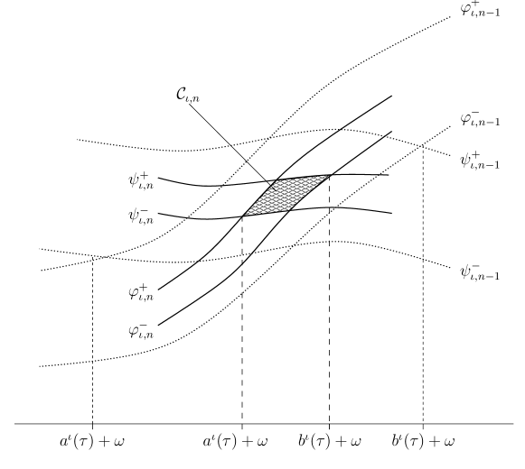
Figure 4.1: The two ‘strips’ $f^{M_{n}}(A^{\iota}_{n})$ and $f^{-M_{n}}(B^{\iota}_{n})$ intersect each other in a transversal way, producing a connected component of ${\cal C}_{n}$.

Using this notation, we can now restate the following estimates from [19].

Proposition 4.4 (Proposition 3.11 and Lemma 3.14 in [19]).

Suppose (${\cal A}1$)–(${\cal A}7$) hold and $({\cal X})_{n}$ and $({\cal Y})_{n}$ are satisfied. Then there exists a constant $\alpha_{1}=\alpha_{1}(s,S)$ such that the following holds: If $\alpha_{\infty}>\alpha_{1}$ then

• ${\cal I}_{n}(\tau)$ and ${\cal I}_{n+1}(\tau)$ consist of exactly ${\cal N}$ connected components and each component of ${\cal I}_{n}(\tau)$ contains exactly one component of ${\cal I}_{n+1}(\tau)$.

• For all connected components of $I^{\iota}_{n+1}(\tau)$ of ${\cal I}_{n+1}(\tau)$ there holds

  (4.7) $$|I^{\iota}_{n+1}(\tau)|\ \leq\ 2\alpha_{\infty}^{-M_{n}}/s\ .$$

• Either

  (4.8) $$\inf_{\theta\in{\cal I}_{n}(\tau)+\omega}\partial_{\theta}\varphi^{\xi}_{\iota,n}(\theta,\tau)-\partial_{\theta}\psi^{\zeta}_{\iota,n}(\theta,\tau)\ > 0 \quad\forall\xi,\zeta\in\{+,-\}\qquad\textrm{or}$$

  (4.9) $$\sup_{\theta\in{\cal I}_{n}(\tau)+\omega}\partial_{\theta}\varphi^{\xi}_{\iota,n}(\theta,\tau)-\partial_{\theta}\psi^{\zeta}_{\iota,n}(\theta,\tau) < 0\quad\forall\xi,\zeta\in\{+,-\}\ .$$

We note that part (iii) can be seen justification for the picture in Figure 4.1, insofar as (4.8), respectively (4.9) ensures that each of the pairs of curves $\varphi^{\xi}_{\iota,n}$ and $\psi^{\zeta}_{\iota,n}$ intersect in exactly one point and $f_{\tau}^{M_{n}}(A^{\iota}_{n})$ crosses $f^{-M_{n}}(B^{\iota}_{n})$ either upwards (as depicted) or downwards.

It remains to obtain a good control on the dependence of the critical regions ${\cal I}_{n}(\tau)$ on $\tau$. This will be the content of the next section. On the technical level, this is the crucial difference in comparison to the construction in [19].

4.2 Dependence of the critical regions on $\tau$.

In order to perform the parameter exclusion with respect to $\tau$, we need to show that different connected components of ${\cal I}_{n}(\tau)$ move with different speed as the parameter $\tau$ changes. This is ensured by the following lemma.

Lemma 4.5.

Suppose (${\cal A}1$)–(${\cal A}10$) hold and $({\cal X})_{n}$ and $({\cal Y})_{n}$ are satisfied. Then there exists a constant $\alpha_{2}=\alpha_{2}(s,S,L,\eta)$ such that the following holds:

If $\alpha_{\infty}>\alpha_{2}$ then all connected components of ${\cal I}_{n+1}(\tau)$ are differentiable in $\tau$. Further,

(4.10) $$|\partial_{\tau}I^{\iota}_{n+1}(\tau)| < 2L/s\qquad\forall\iota\in\{1,\ldots,{\cal N}\}\qquad\textrm{ and }$$

(4.11) $$|D_{\tau}(I^{\iota}_{n+1}(\tau),I^{\kappa}_{n+1}(\tau))| > \frac{\eta}{2}\qquad\qquad\forall\iota\neq\kappa\in\{1,\ldots,{\cal N}\}\ .$$

Proof. We write $I_{n+1}^{\iota}(\tau)=(a^{\iota}(\tau),b^{\iota}(\tau)$ and show that

(4.12) $$\partial_{\tau}a^{\iota}(\tau),\ \partial_{\tau}b^{\iota}(\tau)\ \in\ B_{\Delta}(Q^{\iota}(\tau))\quad\forall\iota\in[1,{\cal N}])$$

where $\Delta:=\min\{\eta/4,L/s\}$. Due to (${\cal A}10$) this immediately implies (4.11). Further, since $Q^{\iota}(\tau)\subseteq[-L/s,L/s]$ by (${\cal A}7$) and (${\cal A}8$) we also obtain (4.10).

We carry out the proof only for $\partial_{\tau}a^{\iota}(\tau)$ since the other endpoint can be treated in the same way. Similarly, we assume that the crossing between $f^{M_{n}}_{\tau}(A^{\iota}_{n})$ and $f^{-M_{n}}_{\tau}(B^{\iota}_{n})$ is upwards, that is, case (4.8) in Proposition 4.4(iii) holds. Again, the other case can be treated similarly. Then, as can be seen from the picture in Figure 4.1, $a^{\iota}(\tau)$ is characterized by the equality

$$\varphi^{+}_{\iota,n}(a^{\iota}(\tau)+\omega,\tau)-\psi^{-}_{\iota,n}(a^{\iota}(\tau)+\omega,\tau)\ =\ 0\ .$$

Application of the Implicit Function Theorem therefore yields

(4.13) $$\partial_{\tau}a^{\iota}(\tau)\ =\ -\ \frac{\partial_{\tau}\left(\varphi^{+}_{\iota,n}-\psi^{-}_{\iota,n}\right)(a(\tau)+\omega,\tau)}{\partial_{\theta}\left(\varphi^{+}_{\iota,n}-\psi^{-}_{\iota,n}\right)(a(\tau)+\omega,\tau)}\ .$$

We start by deriving an estimate on the numerator. Let $\theta:=a^{\iota}(\tau)+\omega$ and $x:=\varphi^{+}_{\iota,n}(\theta,\tau)=f^{M_{n}}_{\tau,\theta-M_{n}\omega}(c^{+})$. Let $\theta_{0}=\theta-M_{n}\omega$ and $\theta_{k}=\theta_{0}+k\omega$. Further, let $x_{0}=c^{+}$ and $x_{k}=f^{k}_{\tau,\theta_{0}}(x_{0})$. Note that thus $(\theta,x)=(\theta_{M_{n}},x_{M_{n}})$. Differentiating with respect to $\tau$ we obtain

(4.14) $$\partial_{\tau}\varphi^{+}_{\iota,n}(\theta,\tau)\ =\ \partial_{\tau}f_{\tau,\theta_{M_{n}-1}}(x_{M_{n}-1})\ +\ \ \underbrace{\sum_{k=1}^{M_{n}-1}\partial_{x}f^{M_{n}-k}_{\tau,\theta_{k}}(x_{k})\cdot\partial_{\tau}f_{\tau,\theta_{k-1}}(x_{k-1})}_{=:r_{1}^{\iota}}\ .$$

Since $\partial_{x}f^{M_{n}-k}_{\tau,\theta_{k}}(x_{k})=\left(\partial_{x}f_{\tau,\theta}^{-M_{n}+k}(x)\right)^{-1}$ and $(\theta,x)\in\mathrm{cl}\left(f_{\tau}({\cal C}_{n})\right)$, the estimate (4.2) in Lemma 4.3 yields $\partial_{x}f^{M_{n}-k}_{\tau,\theta_{k}}(x_{k})\leq\alpha_{\infty}^{-k}$. Together with the upper bound $L$ on the derivative with respect to $\tau$ provided by (${\cal A}8$) we obtain $|r_{1}^{\iota}|\ \leq\ L\cdot\sum_{k=1}^{\infty}\alpha_{\infty}^{-k}$.

Now let $\theta=a^{\iota}(\tau)+\omega$ as before, $\xi=\psi^{-}_{\iota,n}(\theta,\tau)$, $\vartheta_{0}=\theta+M_{n}\omega$, $\vartheta_{k}=\vartheta_{0}+k\omega$,$\xi_{0}=e^{-}$ and $\xi_{k}=f^{k}_{\tau,\vartheta_{0}}(\xi_{0})$. Note that $(\vartheta_{-M_{n}},xi_{-M_{n}})=(\theta,\xi)$. Differentiating with respect to $\tau$ yields

$$r^{\iota}_{2} := \partial_{\tau}\psi^{-}_{\iota,n}(\theta,\tau)\ =\ \sum_{k=1}^{M_{n}}\partial_{x}f_{\tau,\vartheta_{-k}}^{-M_{n}+k}(\xi_{-k})\cdot\partial_{\tau}f^{-1}_{\tau,\vartheta_{-k+1}}(\xi_{-k+1})$$

$$= -\ \sum_{k=1}^{M_{n}}\left(\partial_{x}f^{M_{n}-k}_{\tau,\vartheta_{-M_{n}}}(\xi_{-M_{n}})\right)^{-1}\cdot\left(\partial_{x}f_{\tau,\vartheta_{-k}}(\xi_{-k})\right)^{-1}\cdot\partial_{\tau}f_{\tau,\vartheta_{-k}}(\xi_{-k})$$

$$= -\ \sum_{k=1}^{M_{n}}\left(\partial_{x}f^{M_{n}-k+1}_{\tau,\vartheta_{-M_{n}}}(\xi_{-M_{n}})\right)^{-1}\cdot\partial_{\tau}f_{\tau,\vartheta_{-k}}(\xi_{-k})\ .$$

Using (${\cal A}8$) and (4.2) again we obtain $|r^{\iota}_{2}|\leq L\cdot\sum_{k=1}^{\infty}\alpha_{\infty}^{-k}$. If we let $r^{\iota}=r^{\iota}_{1}-r^{\iota}_{2}$ and use that $\theta_{M_{n}-1}=\theta-\omega$ and $x_{M_{n}-1}=f_{\tau,\theta}^{-1}(x)$ then

(4.16) $$\partial_{\tau}\left(\varphi^{+}_{\iota,n}-\psi^{-}_{\iota,n}\right)(\theta,\tau) = \partial_{\tau}f_{\tau,\theta-\omega}\left(f_{\tau,\theta}^{-1}(x)\right)\ +\ r^{\iota}$$

(4.17) $$\textrm{with }\quad|r^{\iota}| \leq 2L/(\alpha_{\infty}-1)\ .$$

If we replace $\partial_{\tau}$ by $\partial_{\theta}$ in these computations and use (${\cal A}5$) instead of (${\cal A}8$), then we obtain in exactly the same way that

(4.18) $$\partial_{\theta}\left(\varphi^{+}_{\iota,n}-\psi^{-}_{\iota,n}\right)(\theta,\tau) = \partial_{\theta}f_{\tau,\theta-\omega}\left(f_{\tau,\theta}^{-1}(x)\right)\ +\ q^{\iota}$$

(4.19) $$\textrm{with }\quad|q^{\iota}| \leq 2S/(\alpha_{\infty}-1)\ .$$

Now $\theta-\omega\in{\cal I}_{n}\subseteq{\cal I}_{0}$, such that $\left|\partial_{\theta}f_{\tau,\theta-\omega}\left(f_{\tau,\theta}^{-1}(x)\right)\right|>s$ by (${\cal A}7$) and

$$\partial_{\tau}f_{\tau,\theta-\omega}\left(f_{\tau,\theta}^{-1}(x)\right)/\partial_{\theta}f_{\tau,\theta-\omega}\left(f_{\tau,\theta}^{-1}(x)\right)\ \in\ Q^{\iota}(\tau)$$

by the definition of $Q^{\iota}(\tau)$. Furthermore, it follows from the above estimates that $|r^{\iota}|$ and $|q^{\iota}|$ go to zero as $\alpha_{\infty}\to\infty$. Hence, for sufficiently large $\alpha_{\infty}$ we have

(4.20) $$\partial_{\tau}a^{\iota}(\tau)\ =\ -\ \frac{\partial_{\tau}f_{\tau,\theta-\omega}\left(f_{\tau,\theta}^{-1}(x)\right)+r^{\iota}}{\partial_{\theta}f_{\tau,\theta-\omega}\left(f_{\tau,\theta}^{-1}(x)\right)+q^{\iota}}\ \in\ B_{\Delta}(Q^{\iota}(\tau))\ .$$

Furthermore, it can be seen from the above estimates that the largeness condition on $\alpha_{\infty}$ only depends on the constants $s,S,L$ and $\eta$. ∎

4.3 Preliminaries for the parameter exclusion

We now collect some preliminary statements for the parameter exclusion. The setting is an abstract one that does not depend on the previous dynamical construction. We first fix an integer ${\cal N}$ and sequences $(K_{n})_{n\in\mathbb{N}_{0}}$ and $(\epsilon_{n})_{n\in\mathbb{N}_{0}}$ with the same properties as in Section 4.1 and a sequence $(N_{n})_{n\in\mathbb{N}_{0}}$ of positive integers that satisfy

($${\cal N}1 N_{0}\geq 3\quad\textrm{and}\quad N_{n+1}\geq 2K_{n}N_{n}\ \forall n\in\mathbb{N}_{0}\ .$$)

We denote by ${\cal S}(\mathbb{T}^{1})$ the set of all subsets of $\mathbb{T}^{1}$. Let $\Lambda\subseteq[0,1]$ be an open interval. Then we simply assume that we are given a sequence of mappings

$${\cal I}_{n}\ :\quad\Lambda\times\mathbb{N}^{n}\to{\cal S}(\mathbb{T}^{1})\ ,\quad(\tau,M_{0},\ldots,M_{n-1})\ \mapsto\ {\cal I}_{n}(\tau)={\cal I}_{n}(\tau,M_{0},\ldots,M_{n-1})\$$

The dependence of ${\cal I}_{n}(\tau)$ on $M_{0},\ldots,M_{n-1}$ will be kept implicit. We let

$${\cal P}_{n}={\cal P}_{n}(M_{0},\ldots,M_{n})\ :=\ \{\tau\in\Lambda\mid({\cal X^{\prime}})_{n}\textrm{ and }({\cal Y^{\prime}})_{n}\textrm{ hold}\}\ .$$

Here $({\cal X^{\prime}})_{n}$ and $({\cal Y^{\prime}})_{n}$ are understood as conditions on the sets ${\cal I}_{j}(\tau)$ ($j\in[0,n]$) for fixed $\omega\in\mathbb{T}^{1}$. Furthermore, we assume that the following conditions are satisfied.

($$\cal P \left\{\quad\begin{array}[]{l}\textrm{Suppose }M_{0},\ldots,M_{n}\textrm{ with }M_{i}\in[N_{i},2K_{i}N_{i})\ \forall i=[0,n]\textrm{ are fixed.}\\ \textrm{Then for all }\tau\in{\cal P}_{n}(M_{0},\ldots,M_{n})\textrm{ and }j\in[0,n+1]\textrm{ there holds }\\ \\ \begin{array}[]{cl}({\cal P}1)&{\cal I}_{j}(\tau)\textrm{ is open and consists of exactly }{\cal N}\textrm{ connected components }\\ &I^{1}_{j}(\tau),\ldots,I^{\cal N}_{j}(\tau).\textrm{ If }j\leq n\textrm{ then }I^{\iota}_{j+1}(\tau)\subseteq I^{\iota}_{j}(\tau)\ \forall\iota\in[1,{\cal N}].\\ \\ ({\cal P}2)&\textrm{The set }{\cal P}_{j}(M_{0},\ldots,M_{j})\textrm{ is open and all }I^{\iota}_{j}\textrm{ with }j\in[1,{\cal N}]\\ &\textrm{ are differentiable w.r.t.\ }\tau\textrm{ on }{\cal P}_{j}(M_{0},\ldots,M_{j});\\ \\ ({\cal P}3)&|I^{\iota}_{j}(\tau)|\leq\epsilon_{j}\quad\forall\iota\in[1,{\cal N}]\ ;\\ \\ ({\cal P}4)&|\partial_{\tau}I^{\iota}_{j}(\tau)|\leq 2L/s\quad\forall\iota\in[1,{\cal N}]\ ;\\ \\ ({\cal P}5)&|D_{\tau}(I^{\iota}_{j}(\tau),I^{\kappa}_{j}(\tau))|\geq\eta/2\quad\forall\iota\neq\kappa\in[1,{\cal N}]\ ;\end{array}\end{array}\right.$$)

Remark 4.6.

Note that if (${\cal A}1$)–(${\cal A}10$) are satisfied and $\alpha_{\infty}$ is sufficiently large, then the fact that ($\cal P$) holds for the sets ${\cal I}_{j}(\tau)$ defined by (4.1) is exactly the content of the previous sections. $({\cal P}1)$ follows by induction from Proposition 4.4. Lemma 4.5 implies that the connected components of ${\cal I}_{j}$ are differentiable with respect to $\tau$, which in turn yields the openness of the conditions $({\cal X}^{\prime})_{j}$ and $({\cal Y^{\prime}})_{j}$ and hence of ${\cal P}_{j}(M_{0},\ldots,M_{j})$, such that $({\cal P}2)$ holds as well. $({\cal P}3)$ follows from Proposition 4.4 and finally $({\cal P}4)$ and $({\cal P}5)$ are again a consequence of Lemma 4.5.

In each step of the parameter exclusion we will have to ensure that the set ${\cal P}_{n}\setminus{\cal P}_{n+1}$ of excluded parameters is small. In other words, we have to show that for most $\tau\in{\cal P}_{n}$ the conditions $({\cal X}^{\prime})_{n+1}$ and $({\cal Y}^{\prime})_{n+1}$ are satisfied for a suitable $M_{n+1}$ (that we allow to depend on $\tau$). This is greatly simplified by the fact that $({\cal Y})_{n+1}$ ‘comes for free’.

Lemma 4.7 (Lemma 3.16 in [19]).

Suppose that $M_{0},\ldots,M_{n}$ with $M_{j}\in[N_{j},2N_{j})\ \forall j\in[0,n]$ are fixed. Further, assume that (${\cal N}1$), $({\cal P}1)$ and $({\cal P}3)$ hold and

($${\cal K} \sum_{j=0}^{\infty}\frac{1}{K_{j}}\ <\ \frac{1}{6{\cal N}^{2}}\ .$$)

Then for all $\tau\in{\cal P}_{n}(M_{0},\ldots,M_{n})$ there exists an integer $M(\tau)\in[N_{n+1},2N_{n+1})$ such that

(4.21) $$d\left(({\cal I}_{n+1}(\tau)-(M(\tau)-1)\omega)\cup({\cal I}_{n+1}+(M(\tau)+1)\omega)\ ,\ {\cal Y}_{n}\right)\ >\ 3\epsilon_{n}\ .$$

We remark that the version of this lemma in [19] actually contains some additional assumptions, but these are not used in the proof. (For the sake of brevity, the standard hypothesis were assumed throughout the respective section in [19].) In order to obtain an estimate on the set of $\tau\in{\cal P}_{n}$ that do not satisfy $({\cal X})_{n+1}$, the following lemma is needed.

Lemma 4.8.

Suppose $\Lambda\subseteq[0,1]$ is an interval and ${\cal I}:\Lambda\to{\cal S}(\mathbb{T}^{1})$ is such that for all $\tau\in\Lambda$ the set ${\cal I}(\tau)\subseteq\mathbb{T}^{1}$ consists of ${\cal N}$ connected components $I^{1}(\tau),\ldots,I^{\cal N}(\tau)$ of length $|I^{\iota}(\tau)|\leq\delta$ which satisfy

(4.22) $$|D_{\tau}(I^{\iota}(\tau),I^{\kappa}(\tau))|\geq\eta/2\quad\forall\iota\neq\kappa\in[1,{\cal N}]\ .$$

Further, assume that

(4.23) $$d(I^{\iota}(\tau),I^{\iota}(\tau)+n\omega)\ >\ \epsilon\quad\forall\tau\in\Lambda,\ n\in[1,M],\ \iota\in[1,{\cal N}]\ .$$

Then the set

$$\Upsilon\ :=\ \left\{\tau\in\Lambda\ \left|\ d\left({\cal I}(\tau),\bigcup_{j=1}^{M}{\cal I}(\tau)+n\omega\right)\leq\epsilon\right.\right\}$$

has measure $\leq 8{\cal N}^{2}M\frac{\delta+\epsilon}{\eta}$ and consists of at most $2{\cal N}^{2}M-1$ connected components.

Proof. Fix $\iota\neq\kappa\in[1,{\cal N}]$ and $n\in[1,M]$. As $I^{\iota}(\tau)$ and $I^{\kappa}(\tau)$ are disjoint for all $\tau\in\Lambda$ and due to (4.22), the set of $\tau$ with $d\left(I^{\iota}(\tau),(I^{\kappa}(\tau)+n\omega)\right)\leq\epsilon$ consists of at most two intervals of length $\leq 4(\delta+\epsilon)/\eta$. Summing up over all $\iota,\kappa$ and $n$ yields the statement. ∎

For any $n\geq 1$, let

(4.24) $$v_{n} = \ 32{\cal N}^{2}K_{n+1}N_{n+1}\cdot\frac{L}{s\epsilon_{n-1}}\quad\textrm{and}$$

(4.25) $$u_{n} = 1280{\cal N}^{2}K_{n+1}N_{n+1}\cdot\frac{L}{s\eta}\cdot\frac{\epsilon_{n}}{\epsilon_{n-1}}\ .$$

Further, let $v_{0}=8{\cal N}^{2}K_{0}N_{0}$ and $u_{0}=320{\cal N}^{2}K_{0}N_{0}\epsilon_{0}/\eta$.

Lemma 4.9.

Suppose $\omega\in{\cal D}(\sigma,\nu)$, (${\cal N}1$), (${\cal K}$) and ($\cal P$) hold and

($${\cal N}2 10\epsilon_{n}\ <\ \sigma\cdot(4K_{n}N_{n})^{-\nu}\quad\forall n\in\mathbb{N}_{0}\ .$$)

Further, assume that $M_{0},\ldots,M_{n}$ with $M_{j}\in[N_{j},2N_{j})\ \forall j\in[0,n]$ are fixed and $\Gamma\subseteq{\cal P}_{n}(M_{0},\ldots,M_{n})$ is an interval. Then for some $r\leq v_{n+1}$ there exist disjoint intervals $\Gamma_{1},\ldots,\Gamma_{r}\subseteq\Gamma$ and numbers $M^{k}\in[N_{n+1},2N_{n+1}),\ k\in[1,r]$ such that

(4.26) $$\Gamma^{k} \subseteq {\cal P}_{n+1}(M_{0},\ldots,M_{n},M^{k})\quad\textrm{and}$$

(4.27) $$\quad\sum_{k=1}^{r}\mathrm{Leb}(\Gamma^{k}) \geq \mathrm{Leb}(\Gamma)-u_{n+1}\ .$$

Proof. Divide $\Gamma$ into at most $\frac{4L}{s\epsilon_{n}}$ intervals $\Omega_{i}$ of length of length $\leq\frac{s\epsilon_{n}}{2L}$. Denote the midpoint of $\Omega_{i}$ by $\tau_{i}$ and choose $\tilde{M}^{i}=M(\tau_{i})$ according to Lemma 4.7 such that (4.21) holds for $\tau_{i}$. Then due to $({\cal P}4)$ we obtain that $({\cal Y})_{n+1}$ holds for all $\tau\in\Omega^{i}$. Application of Lemma 4.8 with $M=2K_{n+1}\tilde{M}^{i}<4K_{n+1}N_{n+1}$, $\delta=\epsilon_{n+1}$ and $\epsilon=9\epsilon_{n+1}$ yields the existence of a set $\tilde{\Omega}_{i}\subseteq{\cal P}_{n+1}(M_{0},\ldots,M_{n},\tilde{M}^{i})$ of measure $\geq\mathrm{Leb}(\Omega_{i})-320{\cal N}^{2}K_{n+1}N_{n+1}\cdot\frac{\epsilon_{n+1}}{\eta}$ and with at most $8{\cal N}^{2}K_{n+1}N_{n+1}$ connected components. Note that the fact that (4.23) holds follows from the Diophantine condition on $\omega$ together with (${\cal N}2$) and $({\cal P}3)$. Relabelling the connected components of the sets $\tilde{\Omega}_{i}$ and summing up over all $i$ yields the statement. ∎

Let $V_{-1}=1$ and $V_{n}\ =\ \prod_{j=0}^{n}v_{j}$ for $n\geq 0$.

Proposition 4.10.

Suppose $\omega\in{\cal D}(\sigma,\nu)$, $({\cal N}1$-$2)$, (${\cal K}$) and ($\cal P$) hold and

(4.28) $$m\ :=\ \mathrm{Leb}(\Lambda)-\sum_{n=0}^{\infty}V_{n-1}u_{n}.$$

• Then there exists a set $\Lambda_{\infty}\subseteq\Lambda$ of measure $\geq m$ with the following property: For all $\tau\in\Lambda_{\infty}$ there exists a sequence $(M_{n}(\tau))_{n\in\mathbb{N}_{0}}$ with $M_{n}(\tau)\in[N_{n},2N_{n})\ \forall n\in\mathbb{N}$ such that $\tau\in\bigcap_{n\in\mathbb{N}}{\cal P}_{n}(M_{0}(\tau),\ldots,M_{n}(\tau))$.

• If there exists $M_{0}\in[N_{0},2N_{0})$ with ${\cal P}_{0}(N_{0})=\Lambda$, then $\Lambda_{\infty}$ can be chosen with measure $\geq m+u_{0}$.

Proof. We construct a nested sequence of sets $\Lambda_{n}$ with the following properties:

• $\Lambda_{n}$ consists of $\rho_{n}\leq V_{n}$ disjoint intervals $\Lambda^{1}_{n},\ldots,\Lambda^{\rho_{n}}_{n}$;

• $\mathrm{Leb}(\Lambda_{n})\geq\mathrm{Leb}(\Lambda)-\sum_{i=0}^{n}V_{n-1}u_{n}$;

• For each $i\in[1,\rho_{n}]$ there exist numbers $M_{0}^{n,i},\ldots,M_{n}^{n,i}$ such that $\Lambda_{n}^{i}\subseteq{\cal P}_{n}(M_{0}^{n,i},\ldots,M_{n}^{n,i})$;

• For each $k\leq n$ and each $i\in[1,\rho_{n}]$ there exists a unique $\kappa\in[1,\rho_{k}]$ such that $\Lambda^{i}_{n}\subseteq\Lambda^{\kappa}_{k}$ and $M^{n,i}_{j}=M^{k,\kappa}_{j}\ \forall j\in[0,k]$.

The set $\Lambda_{\infty}=\bigcap_{n\in\mathbb{N}_{0}}\Lambda_{n}$ then clearly has the properties required in (a), and for (b) it suffices to note that if ${\cal P}(M_{0})=\Lambda$, then obviously a measure of $u_{0}$ is gained in the first step of the construction.

For $n=0$ we choose $M_{0}\in[N_{0},2N_{0})$ arbitrarily and let $\Lambda_{0}={\cal P}_{0}(M_{0})$. The fact that it has the required properties follows directly from Lemma 4.8. Now suppose that $\Lambda_{0},\ldots,\Lambda_{n}$ with the above properties exist. Then for each $i\in[1,\rho_{n}]$ we can apply Lemma 4.9 and obtain a union of at most $v_{n+1}$ intervals with overall measure $\geq\mathrm{Leb}(\Lambda_{n}^{i})-u_{n+1}$. Doing this for the at most $V_{n}$ components of $\Lambda_{n}$ yields the required set $\Lambda_{n+1}$. ∎

4.4 Minimality and the uniqueness of SNA.

As a first step in the proof of Theorem 3.1 below, we will define the set $\Lambda_{\infty}$ and show that for all $\tau\in\Lambda_{\infty}$ the slow-recurrence conditions $({\cal X^{\prime}})_{n}$ and $({\cal Y^{\prime}})_{n}$ hold. Once this is accomplished, the parameter dependence on $\tau$ does not play a role anymore and we can consider the map $f_{\tau}$ as being fixed. The existence of an SNA and an SNR then follows from Proposition 4.1, and it remains to prove the uniqueness and one-valuedness of the invariant graphs and the minimality of $f$. However, this second step has already been carried out in [19] and the proof given there literally remains true in our setting. Instead of repeating it here, we just give a precise formulation of the formal statement that can be deduced from [19].

Proposition 4.11.

Suppose $f_{\tau}$ satisfies (${\cal A}1$)–(${\cal A}7$), $({\cal X})_{n}$ and $({\cal Y})_{n}$ hold for all $n\in\mathbb{N}$ and

(4.29) $$\mathrm{Leb}\left(\bigcup_{n=0}^{\infty}\bigcup_{k=-M_{n}-1}^{M_{n}+1}{\cal I}_{n}-k\omega\right)\ <\ \frac{1}{4+4p^{2}}\ .$$

Then $f_{\tau}$ has a unique SNA and SNR which are both one-valued. Further the dynamics are minimal.

Proof. See Sections 3.6 and 3.7 in [19]. ∎

4.5 Proof of Theorem 3.1.

Fix an integer $t\geq 4$ such that $2^{-t+2}/{\cal N}^{2}\leq\log((p^{2}+2)/(p^{2}+1))$ and let $K_{n}=2^{n+t}{\cal N}^{2}$. Then it is easy to check that (${\cal K}$) is verified and furthermore $\beta$ in (4.1) is larger than $(p^{2}+1)/(p^{2}+2)$. This in turn implies that $\alpha_{\infty}$ defined by (4.1) is larger than $\alpha^{1/p}$. Suppose that (${\cal A}1$)–(${\cal A}10$) hold and $\alpha^{1/p}>\max\{\alpha_{1},\alpha_{2}\}$, where $\alpha_{1}$ and $\alpha_{2}$ are the constants from Proposition 4.4 and Lemma 4.5. Then as mentioned in Remark 4.6, the critical regions ${\cal I}_{n}$ defined dynamically by (4.1) satisfy ($\cal P$) when viewed as mappings ${\cal I}_{n}:\Lambda\times\mathbb{N}^{n}\to{\cal S}(\mathbb{T}^{1})$. In order to determine the set $\Lambda_{\infty}$ by applying Proposition 4.10, it only remains to show that by an appropriate choice of the sequences $(\epsilon_{n})_{n\in\mathbb{N}_{0}}$ and $(N_{n})_{n\in\mathbb{N}_{0}}$ we can ensure that (${\cal N}1$) and (${\cal N}2$) hold and that the sum $\sum_{n=0}^{\infty}V_{n-1}u_{n}$ in (4.28) is smaller than $\delta$.

In order to do so, we let $N_{0}=3$ and $N_{n+1}=\alpha^{N_{n}/qp}$, where $q=\max\{8,2\nu\}$. Further, we let $\epsilon_{0}=\sup_{\iota\in[1,{\cal N}],\tau\in\Lambda}|I^{\iota}_{0}(\tau)|$ and $\epsilon_{n+1}=\frac{2}{s}\cdot\alpha^{-N_{n}/p}$. Note that these sequences grow, respectively decay, super-exponentially. Therefore it is easy to see that with this choice (${\cal N}1$) and (${\cal N}2$) are satisfied for sufficiently large $\alpha$ and sufficiently small $\epsilon_{0}$. In the following estimates we assume that $\alpha$ is chosen sufficiently large and indicate the steps in which this fact is used by placing $(\alpha)$ over the respective inequality signs. For any $n\in\mathbb{N}_{0}$ we have

$$v_{n+1} = 32{\cal N}^{2}K_{n+1}N_{n+1}\cdot\frac{L}{s\epsilon_{n}}$$

$$= 16\cdot 2^{n+t}{\cal N}^{2}L\cdot\alpha^{N_{n}/qp+N_{n-1}/p}\ \stackrel{{\scriptstyle(\alpha)}}{{\leq}}\ \alpha^{N_{n}/4}\quad\textrm{and}$$

$$u_{n+1} = 1280{\cal N}^{2}K_{n+1}N_{n+1}\cdot\frac{L}{s\eta}\cdot\frac{\epsilon_{n+1}}{\epsilon_{n}}$$

$$= 1280\cdot 2^{n+t}{\cal N}^{2}\cdot\frac{L}{s\eta}\cdot\alpha^{N_{n}/qp+N_{n-1}/p-N_{n}/p}\ \stackrel{{\scriptstyle(\alpha)}}{{\leq}}\ \alpha^{-3N_{n}/4p}\ .$$

By induction, we obtain that $V_{n}=\prod_{j=0}^{n}v_{j}\stackrel{{\scriptstyle(\alpha)}}{{\leq}}\alpha^{N_{n}/4}$ (note that $v_{0}=8{\cal N}^{2}K_{0}N_{0}\stackrel{{\scriptstyle(\alpha)}}{{\leq}}\alpha^{N_{0}/4}$). Altogether, this yields that $m$ in Proposition 4.10 satisfies $m\geq\mathrm{Leb}(\Lambda)-u_{0}-\sum_{n=0}^{\infty}\alpha^{-N_{n}/2p}$. As $u_{0}=320{\cal N}^{2}K_{0}N_{0}\epsilon_{0}/\eta$, this lower bound goes to $\mathrm{Leb}(\Lambda)$ as $\epsilon_{0}\to 0$ and $\alpha\to\infty$.

Hence, Proposition 4.10 yields the existence of a set $\Lambda_{\infty}\subseteq\Lambda$ of measure $\mathrm{Leb}(\Lambda_{\infty})>\mathrm{Leb}(\Lambda)-\delta$ such that for all $\tau\in\Lambda_{\infty}$ the conditions $({\cal X^{\prime}})_{n}$ and $({\cal Y^{\prime}})_{n}$ are satisfied. Fix $\tau\in\Lambda_{\infty}$. As $\alpha_{\infty}>1$ and ${\cal I}_{n}(\tau)\neq\emptyset\ \forall n\in\mathbb{N}$ due to $({\cal P}1)$, Proposition 4.1 yields the existence of an SNA and an SNR. Further, we have

$$\mathrm{Leb}\left(\bigcup_{n=0}^{\infty}\bigcup_{k=-M_{n}-1}^{M_{n}+1}{\cal I}_{n}-k\omega\right) \leq \sum_{n=0}^{\infty}4N_{n}\epsilon_{n}\ \leq\ \epsilon_{0}N_{0}+\sum_{n=1}^{\infty}\alpha^{-N_{n}/2p}\ .$$

Again, the right side goes to $\mathrm{Leb}(\Lambda)$ as $\epsilon_{0}\to 0$ and $\alpha\to\infty$, such that (4.29) will be satisfied for small $\epsilon_{0}$ and large $\alpha$. Consequently, we can apply Proposition 4.11 to obtain $(*)$ ‣ 3.1 for all $\tau\in\Lambda_{\infty}$.

Finally, suppose that for some $\tau_{0}$ the symmetry condition (3.2) holds. In this situation it follows by induction that the critical regions ${\cal I}_{n}=I^{1}_{n}\cup I^{2}_{n}$ defined recursively by (4.1) satisfy

(4.30) $$I_{n}^{2}\ =\ I^{1}_{n}+\frac{1}{2}\qquad\forall n\in\mathbb{N}\ .$$

We show that in this case, for all sufficiently large $\alpha$, there exists a sequence of integers $M_{n}\in[N_{n},2N_{n})$ such that the $({\cal X^{\prime}})_{n}$ and $({\cal Y^{\prime}})_{n}$ hold for all $n\in\mathbb{N}$. As before, Proposition 4.1 and Proposition then imply $(*)$ ‣ 3.1, such that $\tau\in\Lambda_{\infty}$.

$({\cal X}^{\prime})_{0}$ with $M_{0}=N_{0}=3$ holds for small $\epsilon_{0}$ due to the Diophantine condition and $({\cal Y}^{\prime})_{0}$ is void. Suppose $M_{0},\ldots,M_{n}$ are chosen such that $({\cal X^{\prime}})_{n}$ and $({\cal Y^{\prime}})_{n}$ hold, such that $\tau\in{\cal P}_{n}(M_{0},\ldots,M_{n})$. Then due to Lemma 4.7 there exists $M_{n+1}\in[N_{n+1},2N_{n+1})$ such that $({\cal Y}^{\prime})_{n+1}$ holds. Furthermore $|I^{\iota}_{n+1}(\tau)|\leq\epsilon_{n+1}$ for $\iota=1,2$ due to $({\cal P}3)$. Now suppose that $({\cal X}^{\prime})_{n+1}$ is not satisfied, such that $I^{\iota}_{n+1}(\tau)\cap(I^{\kappa}_{n+1}(\tau)+n\omega)\neq\emptyset$ for some $\iota,\kappa\in\{1,2\}$ and $|n|\leq 2K_{n+1}M_{n+1}$. Due to (4.30) this implies $d(2n\omega,0)\leq 2\epsilon_{n+1}$, which contradicts the Diophantine condition (${\cal A}0$) when $\alpha$ is large. Consequently, when $\epsilon_{0}$ is sufficiently small and $\alpha$ is sufficiently large conditions $({\cal X^{\prime}})_{n}$ and $({\cal Y^{\prime}})_{n}$ hold for all $n\in\mathbb{N}$ and we can apply Proposition 4.11 to deduce that $f_{\tau_{0}}$ satisfies $(*)$ ‣ 3.1. Hence, $\tau_{0}$ can be included in $\Lambda_{\infty}$. ∎

5 The refined version of the twist parameter exclusion

The aim of this section is to prove Theorem 3.2. To that end, we have to improve some of the estimates from the previous section by taking into account the stronger assumptions on $\partial_{\theta}f_{\theta}$ in (${\cal A}8^{\prime}$) and (${\cal A}9^{\prime}$). As before, we can rely to some extent on the respective results from [19].

5.1 Estimates on the critical sets and critical regions.

Parts (i) and (ii) of Proposition 4.4 are replaced by the following statements, which can again be taken from [19].

Proposition 5.1 (Proposition 4.3 in [19]).

Suppose (${\cal A}1$)–(${\cal A}7$), (${\cal A}9^{\prime}$) and (3.3)–(3.6) hold, $({\cal X})_{n}$ and $({\cal Y})_{n}$ are satisfied, $\alpha_{\infty}>1$ and $M_{0}\geq d^{1/4}$. Then there exist a constant $d_{1}=d_{1}(\alpha_{\infty})>0$ such that the following holds: If $d>d_{1}$ then

• ${\cal I}_{n}(\tau)$ and ${\cal I}_{n+1}(\tau)$ consist of exactly ${\cal N}$ connected components and each component of ${\cal I}_{n}(\tau)$ contains exactly one component of ${\cal I}_{n+1}(\tau)$.

• For all connected components of $I^{\iota}_{n+1}(\tau)$ of ${\cal I}_{n+1}(\tau)$ there holds $|I^{\iota}_{n+1}(\tau)|\leq 2\alpha_{\infty}^{-M_{n}}/s$.

In contrast to this, the required version of Proposition 4.4(iii) has to take into account the fact that due to (${\cal A}7^{\prime}$) only two critical regions exist. This assumption is not considered in [19], such that we cannot use the respective estimates there. Instead, we use the following statement.

Lemma 5.2.

Suppose (${\cal A}1$)–(${\cal A}6$), (${\cal A}7^{\prime}$)–(${\cal A}9^{\prime}$) and (3.3)–(3.6) hold, $({\cal X})_{n}$ and $({\cal Y})_{n}$ are satisfied, $\alpha_{\infty}>1$ and $M_{0}\geq d^{1/4}$. Then there exist a constant $d_{2}=d_{2}(\alpha_{\infty})>0$ such that the following holds. If $d>d_{2}$ then

(5.1) $$s/2 \leq \partial_{\theta}(\varphi_{1,n}^{\pm}-\psi_{1,n}^{\mp})\ \leq\ 2S\qquad\ \ \textrm{ on }I^{1}_{n}(\tau)+\omega\ \textrm{ and }$$

(5.2) $$-2S \leq \partial_{\theta}(\varphi_{2,n}^{\pm}-\psi_{2,n}^{\mp})\ \leq\ -s/2\qquad\textrm{ on }I^{2}_{n}(\tau)+\omega\ .$$

Proof. As in the proof of Lemma 4.5 and with the notation introduced there, we have

(5.3) $$\partial_{\theta}\varphi^{\pm}_{\iota,n}(\theta,\tau)\ =\ \partial_{\theta}f_{\tau,\theta_{M_{n}-1}}(x_{M_{n}-1})+\underbrace{\sum_{k=1}^{M_{n}-1}\partial_{x}f^{M_{n}-k}_{\tau,\theta_{k}}(x_{k})\cdot\partial_{\theta}f_{\tau,\theta_{k-1}}(x_{k-1})}_{=:q^{\iota}_{1}}\ .$$

As $(\theta_{M_{n}},x_{M_{n}})=(\theta,\varphi^{\pm}_{\iota,n}(\theta,\tau))\in{\cal I}_{0}+\omega$, we can use (${\cal A}9^{\prime}$) together with (4.2) and (${\cal A}5$) to obtain

(5.4) $$|q_{1}^{\iota}|\ \leq\ \frac{s^{\prime}+\alpha_{\infty}^{-M_{0}}S}{\alpha_{\infty}-1}\ .$$

For $q^{\iota}_{2}:=\partial_{\theta}\psi^{\mp}_{\iota,n}(\theta,\tau)$ we obtain in a similar way

(5.5) $$|q^{\iota}_{2}|\ \leq\ \frac{s^{\prime}+\alpha_{\infty}^{-M_{0}}S}{\alpha_{\infty}-1}\ .$$

Since $M_{0}\geq d^{1/4}$ we obtain that $|q^{\iota}_{1}|$ and $|q^{\iota}_{2}|$ are small compared to $s$ and $S$ if $d$ is sufficiently large and $\frac{s^{\prime}}{s}$ is sufficiently small. As $\theta_{M_{n}-1}\in{\cal I}_{0}$, the statement follows from (${\cal A}5$) and (${\cal A}8^{\prime}$). ∎

In order to control the parameter dependence of the critical sets we replace Lemma 4.5 by

Lemma 5.3.

Suppose (${\cal A}1$)–(${\cal A}6$), (${\cal A}7^{\prime}$)–(${\cal A}9^{\prime}$) and (3.3)–(3.5) hold and $({\cal X})_{n}$ and $({\cal Y})_{n}$ are satisfied. Further, let $d_{2}$ be chosen as in Lemma 5.2 and assume that $d>d_{2}$. Then

(5.6) $$\partial_{\tau}I_{n+1}^{1}(\tau)\ \leq\ \frac{-\gamma}{2S} \ ,\ \partial_{\tau}I^{2}_{n+1}(\tau)\ \geq\ \frac{\gamma}{2S}$$

(5.7) $$\textrm{ and }\quad|\partial_{\tau}I^{\iota}_{n+1}(\tau)| \leq \frac{4L}{s(1-1/\alpha_{\infty})}\quad(\iota=1,2)\ .$$

Proof. Similar to the proof of Lemma 4.5 we let $I^{\iota}_{n+1}(\tau)=(a^{\iota}(\tau),b^{\iota}(\tau))$ and show that

(5.8) $$-4L/s(1-1/\alpha_{\infty})\ \leq\ \partial_{\tau}a^{1}(\tau)\ \leq-\gamma/2S\ .$$

The required estimates on $\partial_{\tau}b^{1}(\tau),\ \partial_{\tau}a^{2}(\tau)$ and $\partial_{\tau}b^{2}(\tau)$ can then be treated in the same way. Note that (5.1) in Lemma 5.2 implies that $f^{M_{n}}(A^{1}_{n})$ crosses $f^{-M_{n}}(B^{1}_{n})$ upwards.

We define $r^{\iota}_{1}$ and $r^{\iota}_{2}$ as in (4.14) and (4.2). From (4.14) and (${\cal A}8^{\prime}$) we obtain that

(5.9) $$\partial_{\tau}\varphi^{+}_{\iota,n}(\theta,\tau)\ =\ \partial_{\tau}f_{\tau,\theta_{M_{n}-1}}(x_{M_{n}-1})+r^{\iota}_{1}\ \geq\ \partial_{\tau}f_{\tau,\theta_{M_{n}-1}}(x_{M_{n}-1})\ \geq\ \gamma\ .$$

Note that $r^{1}_{1}\geq 0$ since all terms in the sum in (4.14) are non-negative. Similarly $r^{1}_{2}\leq 0$, such that

(5.10) $$\partial_{\tau}(\varphi^{+}_{1,n}-\psi^{-}_{1,n})(a^{1}(\tau)+\omega,\tau)\ \geq\ \gamma\ .$$

Using (4.13) and Lemma 5.2 gives $\partial_{\tau}a^{1}(\tau)\leq-\gamma/2S$ as required.

For the upper bound on $|\partial_{\tau}a^{1}(\tau)|$, note that using (${\cal A}8^{\prime}$) and Lemma 4.3 to estimate the sums defining $r^{1}_{1}$ and $r^{2}_{1}$ in (4.14) and (4.2) yields

(5.11) $$\partial_{\tau}(\varphi^{+}_{1,n}-\psi^{-}_{1,n})(a^{1}(\tau)+\omega,\tau)\ \leq\ 2L/(1-1/\alpha_{\infty})\ .$$

Together with Lemma 5.2, this provides the required bound $|\partial_{\tau}a^{1}(\tau)|\leq 4L/s(1-1/\alpha_{\infty})$. ∎

Remark 5.4.

The proof of Lemma 5.3 demonstrates well the restrictions which the need for controlling the relative speed of the critical intervals inflicts on the geormetry of the forcing. Considering the case of only two critical intervals with opposite sign of the slope of $\partial_{\theta}f_{\theta}$, as we do here, is not the only possibility to achive this. For instance, one could treat a multitude of critical intervals, as in Theorem 3.1, by requiring that the twist $\partial_{\tau}f_{\theta}(x)$ almost vanishes outside of the critical regions (similar to the use of (${\cal A}9^{\prime}$) in the proof of Lemma 5.2). However, we see no way of treating more than two critical intervals if the twist is uniform as in (1.3). The reason is that the lack of strong hyperbolicity does not allow to control the influence of the twist far from the critical region ${\cal I}_{0}(\tau)$ on the relative speed of the critical intervals. This could result in critical intervals moving at the same speed, in which case parameter exclusion would not work anymore.

5.2 Proof of Theorem 3.2.

We choose $t$ and $K_{n}=2^{n+t}/{\cal N}^{2}$ as in the proof of Theorem 3.1, such that $\alpha_{\infty}\geq\alpha^{1/p}>1$. Further, we suppose that $d$ satisfies $d\geq\max\{d_{1},d_{2}\}$, where $d_{1}$ and $d_{2}$ are the constants from Proposition 5.1 and Lemma 5.2. Then the mapping ${\cal I}_{n}:\Lambda\times\mathbb{N}\to{\cal S}(\mathbb{T}^{1})$ satisfies ($\cal P$), with $L$ replaced by $4L/(1-1/\alpha_{\infty})$ due to the weaker estimate on $|\partial_{\tau}I^{\iota}_{n}(\tau)|$ in (5.6) (compare Remark 4.6).

Fix $k>2\nu$ and let $N_{0}$ be the first integer $\geq d^{1/k}$. As before, we let $q=\max\{8,2\nu\}$ and define the sequences $N_{n}$ and $\epsilon_{n}$ recursively by $N_{n+1}=\alpha^{N_{n}/qp}$ and $\epsilon_{n+1}=\frac{2}{s}\cdot\alpha^{-N_{n}/p}$. Then using the dependencies (3.3)–(3.6) it is easy to check that all estimates on the quantities $v_{n},\ u_{n}$ and $V_{n}$ made in the proof of Theorem 3.1 remain valid if the largeness assumption on $\alpha$ used there is replaced by a largeness condition on $d$ that depends on the constants $\alpha,p,L,\gamma,A$ and $\delta$. Consequently, the constant $m$ in Proposition 4.10 satisfies

(5.12) $$m\ \geq\ \mathrm{Leb}(\Lambda)-u_{0}-\sum_{n=0}^{\infty}\alpha^{-N_{n}/2p}\ .$$

Furthermore, since $I^{1}_{0}(\tau)=I^{2}_{0}(\tau)+\frac{1}{2}$, $|I_{0}^{\iota}(\tau)|\leq\epsilon_{0}\leq A/\sqrt{d}$ by (3.5) and $N_{0}\leq d^{1/k}+1$, the Diophantine condition implies that for sufficiently large $d$ condition $({\cal X}^{\prime})_{0}$ holds for all $\tau\in\Lambda$ (that is, ${\cal I}_{0}(\tau)$ is disjoint from its first $2K_{0}N_{0}$ iterates). This means that ${\cal P}(N_{0})=\Lambda$ and we can therefore apply Proposition 4.10(b), which yields a set $\Lambda_{\infty}$ of measure

$$\mathrm{Leb}(\Lambda_{\infty})\ \geq\ \mathrm{Leb}(\Lambda)-\sum_{n=0}^{\infty}\alpha^{-N_{n}/2p}\$$

on which the slow-recurrence conditions $({\cal X^{\prime}})_{n}$ and $({\cal Y^{\prime}})_{n}$ hold for all $n\in\mathbb{N}$. Consequently, for all $\tau\in\Lambda_{\infty}$ the existence of an SNA and an SNR follows from Proposition 4.1. Further, we have

$$\mathrm{Leb}\left(\bigcup_{n=0}^{\infty}\bigcup_{k=-M_{n}-1}^{M_{n}+1}{\cal I}_{n}-k\omega\right) \leq \sum_{n=0}^{\infty}2N_{n}\epsilon_{n}\ \leq\ \epsilon_{0}N_{0}+\frac{2}{s}\cdot\sum_{n=1}^{\infty}\alpha^{-N_{n}/2p}\ .$$

Due to (3.5) and the choice of $N_{0}$ in $[d^{1/k},d^{1/k}+1]$ the sum on the right goes to zero as $d\to\infty$, and we can apply Proposition 4.11 to obtain $(*)$ ‣ 3.1. Finally, the symmetry statement is shown in the same way as in the proof of Theorem 3.1. ∎

5.3 Proof of Corollaries 1.3 and 1.4.

Recall that we consider the parameter family

$$f_{a,b,\tau}(\theta,x)\ =\ \left(\theta+\omega,x+\tau+\frac{a}{2\pi}\sin(2\pi x)+g_{b}(\theta)\right)\$$

with $g_{b}(\theta)=\arctan(b\sin(2\pi\theta))/\pi$. We suppose that $\omega$ is Diophantine with constants $\sigma,\nu$, such that (${\cal A}0$) holds. Let $h_{a}(x)=x+\frac{a}{2\pi}\sin(2\pi x)$. Then there exist constants $0<e<c<\frac{1}{2}$ $\alpha>1,\ p\in\mathbb{N}$ and $0<t<\frac{1}{2}-c$ such that there holds

(5.13) $$h_{a}\left([e,-e]\right) \subseteq (c+t,-c-t)\ ,$$

(5.14) $$h_{a}^{\prime}(x) < \alpha^{-2/p}\qquad\forall x\in C:=[c,-c]\ ,$$

(5.15) $$h_{a}^{\prime}(x) > \alpha^{2/p}\qquad\forall x\in E:=[-e,e]\quad\textrm{and}$$

(5.16) $$\alpha^{-p} < h_{a}^{\prime}(x)\ <\ \alpha^{p}\qquad\forall x\in\mathbb{T}^{1}\ .$$

Let $\Lambda:=\left(\frac{1}{2}-\frac{t}{2},\frac{1}{2}+\frac{t}{2}\right)$ and $\gamma_{0}:=\frac{1}{4}\tan(\pi(\frac{1}{2}-\frac{t}{2}))$. Further, define $I^{1}_{0}:=\left(-\gamma_{0}/b,\gamma_{0}/b\right)$ and $I^{2}_{0}:=I^{1}_{0}+\frac{1}{2}$. Then for $\theta\notin{\cal I}_{0}=I^{1}_{0}\cup I^{2}_{0}$ and $\tau\in\Lambda$ we obtain

$$\textstyle d(g_{b}(\theta)+\tau,0)\ \leq\ \frac{t}{2}+d(g_{b}(\theta),\frac{1}{2})\ <t\ .$$

Consequently $f_{a,b,\tau}$ satisfies (${\cal A}1$)–(${\cal A}4$) for all $\tau\in\Lambda$. Further, we have

$$\partial_{\theta}f_{\theta}(x) = \partial_{\theta}g_{b}(\theta)\ =\ \frac{2}{1+b^{2}\sin^{2}(2\pi\theta)}\cdot b\cos(2\pi\theta)\ \leq\ 2b\qquad\forall(\theta,x)\in\mathbb{T}^{2}\quad\textrm{and}$$

$$|\partial_{\theta}f_{\theta}(x)| \geq \frac{b}{1+(2\pi\gamma_{0})^{2}}\qquad\forall(\theta,x)\in{\cal I}_{0}\times\mathbb{T}^{1}\ .$$

This allows to see that (${\cal A}5$), (${\cal A}6$), (${\cal A}7^{\prime}$) and (${\cal A}8^{\prime}$) are satisfied with $S=2b$ and $s=\frac{b}{1+(2\pi\gamma_{0})^{2}}$. If we let $I^{1^{\prime}}_{0}=[-\gamma_{0}/\sqrt{b},\gamma/\sqrt{b}]$, $I^{2}_{0}=I^{1^{\prime}}_{0}+\frac{1}{2}$ and ${\cal I}_{0}^{\prime}=I^{1^{\prime}}_{0}\cup I^{2^{\prime}}_{0}$ then

$$|\partial_{\theta}f_{\theta}(x)|\ \leq\ 2\gamma_{0}^{-2}\qquad\forall(\theta,x)\in(\mathbb{T}^{1}\setminus{\cal I}_{0}^{\prime})\times\mathbb{T}^{1}\ ,$$

such that (${\cal A}9^{\prime}$) holds with $s^{\prime}=2\gamma_{0}^{-2}$. Finally, since $\partial_{\tau}f_{\theta}(x)=1$, we may choose $\gamma=\frac{1}{2}$ and $L=2$ in (${\cal A}10^{\prime}$). Altogether, this implies that all assumptions of Theorem 3.2 are satisfied for a suitable constant $A$ and $d=b$. The conclusions of the corollaries follow. ∎

References

- [1] M. Benedicks and L. Carleson. The dynamics of the Hénon map. Ann. Math. (2), 133(1):73–169, 1991.
- [2] J. Milnor. On the concept of attractor. Commun. Math. Phys., 99:177–195, 1985.
- [3] C. Grebogi, E. Ott, S. Pelikan, and J.A. Yorke. Strange attractors that are not chaotic. Physica D, 13:261–268, 1984.
- [4] G. Keller. A note on strange nonchaotic attractors. Fundam. Math., 151(2):139–148, 1996.
- [5] F.J. Romeiras, A. Bondeson, E. Ott, T.M. Antonsen Jr., and C. Grebogi. Quasiperiodically forced dynamical systems with strange nonchaotic attractors. Physica D, 26:277–294, 1987.
- [6] M. Ding, C. Grebogi, and E. Ott. Evolution of attractors in quasiperiodically forced systems: From quasiperiodic to strange nonchaotic to chaotic. Phys. Rev. A, 39(5):2593–2598, 1989.
- [7] U. Feudel, J. Kurths, and A. Pikovsky. Strange nonchaotic attractor in a quasiperiodically forced circle map. Physica D, 88:176–186, 1995.
- [8] V.M. Millions̆c̆ikov. Proof of the existence of irregular systems of linear differential equations with quasi periodic coefficients. Differ. Uravn., 5(11):1979–1983, 1969.
- [9] R.E Vinograd. A problem suggested by N.R. Erugin. Differ. Uravn., 11(4):632–638, 1975.
- [10] M. Herman. Une méthode pour minorer les exposants de Lyapunov et quelques exemples montrant le caractère local d’un théorème d’Arnold et de Moser sur le tore de dimension 2. Comment. Math. Helv., 58:453–502, 1983.
- [11] A. Avila and R. Krikorian. Reducibility or non-uniform hyperbolicity for quasiperiodic Schrödinger cocycles. Ann. Math. (2), 164:911–940, 2006.
- [12] A. Haro and J. Puig. Strange non-chaotic attractors in Harper maps. Chaos, 16, 2006.
- [13] J. Puig. Cantor spectrum for the almost Mathieu operator. Comm. Math. Phys., 244(2):297–309, 2004.
- [14] A. Avila and S. Jitomirskaya. The Ten Martini Problem. Ann. Math. (2), 170(1):303–342, 2009.
- [15] A. Avila and S. Jitomirskaya. Almost localization and almost deducibility. J. Eur. Math. Soc., 12(1):93–131, 2010.
- [16] A. Avila. Global theory of one-frequency Schrödinger operators I and II. Preprints 2010.
- [17] L.-S. Young. Lyapunov exponents for some quasi-periodic cocycles. Ergodic Theory Dyn. Syst., 17:483–504, 1997.
- [18] K. Bjerklöv. Positive Lyapunov exponent and minimality for a class of one-dimensional quasi-periodic Schrödinger equations. Ergodic Theory Dyn. Syst., 25:1015–1045, 2005.
- [19] T. Jäger. Strange non-chaotic attractors in quasiperiodically forced circle maps. Comm. Math. Phys., 289(1):253–289, 2009.
- [20] T. Jäger. The creation of strange non-chaotic attractors in non-smooth saddle-node bifurcations. Mem. Am. Math. Soc., 945:1–106, 2009.
- [21] K. Bjerklöv and T. Jäger. Rotation numbers for quasiperiodically forced circle maps – Mode-locking vs strict monotonicity. J. Am. Math. Soc., 22(2):353–362, 2009.
- [22] J. B\a’ellissard and B. Simon. Cantor spectrum for the almost Mathieu equation. J. Funct. Anal., 48(3):408–419, 1982.
- [23] J. Stark, U. Feudel, P. Glendinning, and A. Pikovsky. Rotation numbers for quasi-periodically forced monotone circle maps. Dyn. Syst., 17(1):1–28, 2002.