Energy spectrum and broken spin-surface locking in topological insulator quantum dots

Abstract

We consider the energy spectrum and the spin-parity structure of the eigenstates for a quantum dot made of a strong topological insulator. Using the effective low-energy theory in a finite-length cylinder geometry, numerical calculations show that even at the lowest energy scales, the spin direction in a topologically protected surface mode is not locked to the surface. We find “zero-momentum” modes, and subgap states localized near the “caps” of the dot. Both the energy spectrum and the spin texture of the eigenstates are basically reproduced from an analytical surface Dirac fermion description. Our results are compared to microscopic calculations using a tight-binding model for a strong topological insulator in a finite-length nanowire geometry.

I Introduction

The theoretical prediction and subsequent experimental verification of the conducting surface state of a strong topological insulator (TI) continues to generate a lot of excitement in physics; for reviews, see Refs. hasan, ; qi, ; joel, . In a TI, strong spin-orbit couplings and band inversion conspire to produce a time-reversal invariant topological state different from a conventional band insulator. Using Bi₂Se₃ as a weakly correlated reference TI material with rather large bulk gap $\Delta_{b}\approx 0.3$ meV, surface probe experiments have provided strong evidence for the topologically protected gapless surface state.xia The measured spin texture of the surface state is consistent with predictions obtained for two-dimensional (2D) massless Dirac fermions. Under this “relativistic” description, the spin direction is locked to the surface, and the surface state is stable against the effects of weak disorder and weak interactions (topological protection).hasan ; qi ; joel It is thus useful to first study the simplest case of a noninteracting disorder-free model, which is the case investigated below.

Because of the residual bulk conductivity of the presently available (nominally insulating) TI samples, it has been difficult to experimentally extract the surface contribution to the electrical conductivity. One attempt to improve the situation is to consider mesoscopic samples, where the surface-to-volume ratio is more advantageous. In particular, thin-film geometriesqu ; checkelsky and quasi-1D nanowires (“ribbons”)peng ; cha ; zuev ; tang have been studied experimentally. Signatures for Aharonov-Bohm interference effects associated with the topological surface state in Bi₂Se₃ nanowires were reported,peng cf. also related experiments for Sb₂Te₃ nanowires.zuev For infinitely long and circulary symmetric topological nanowires, band structure calculations predict a multi-channel waveguide where all surface modes are gapped because of spin-surface locking.ashv0 ; egger ; piet ; ashvin With $k$ denoting the conserved momentum along the wire axis (taken along the $z$ direction), and $j$ the half-integer total angular momentum, the dispersion relation of these modes is

$$E_{j,\pm}(k)=\pm\sqrt{(v_{1}k)^{2}+(jv_{2}/R)^{2}},$$ (1)

where $\hbar=1$ throughout and $\pm$ for conduction and valence band, respectively. The Fermi velocities $v_{1}$ and $v_{2}$ differ because the bulk dispersion relation is anisotropic, see below, and the nanowire radius is $R$. Note that there is a minimal gap $\Delta_{s}=v_{2}/R$ for the surface modes since $j$ is half-integer. For reasonable values of $R$, we have $\Delta_{s}\ll\Delta_{b}$.

Experiments probing quantum dot physics in finite-length TI nanowires are expected to yield new insights into the exciting physics of TIs, in close analogy to semiconductor nanowires and carbon nanotubes where such experiments have been highly successful.nano1 ; nano2 To prepare the ground, we here consider the band structure for TI quantum dots with a finite-length nanowire geometry. For a spherical TI dot, the band structure was worked out before.dhlee ; paco ; malkova However, we draw attention to several features that only arise when the surface contains sharp edges, i.e., non-differentiable parts, as is the case for the cylinder. We employ three different and independent approaches to understand TI quantum dot energy levels and their spin texture: (1) For a cylindrical TI nanowire of length $L$ and radius $R$ closed by flat caps, we have performed detailed numerical calculations for the energy spectrum and the spin texture of the eigenstates based on the effective low-energy theory of Zhang et al.;zhang1 ; zhang2 material parameters were chosen for Bi₂Se₃ as quoted in Ref. zhang2, . (2) An analytical approach starting from a surface Dirac fermion description has been developed for the same geometry. Most of our numerical results can thereby be quantitatively reproduced within an analytical theory. (3) We have also studied a microscopic tight-binding model for a strong TI in the finite-size nanowire geometry and find qualitatively similar results.

The main conclusions reached from these three approaches are as follows: First, longitudinal momentum quantization implies a discrete sequence of energy levels which can (roughly) be approximated by letting $k\to k_{n}=n\pi/L$ ($n\in\mathbb{N}$) in Eq. (1). Remarkably, in addition we find unconventional “zero-momentum” states (where, formally, $k_{n}=0$). In such a state, the charge and spin densities are almost homogeneous along the $z$-direction. Furthermore, there are subgap states energetically located within the surface mode gap ($\Delta_{s}$). These states are localized near both caps and show interesting spin texture. Second, we observe significant out-of-surface components for the spin density associated with all energy eigenstates. Note that an out-of-plane spin texture is only expected when trigonal warping effects are important,fu ; yazyev see also very recent experimental results reporting such features.trig1 ; trig2 However, to lowest order in momentum (around the $\Gamma$ point), trigonal warping can be neglected, while we persistently find broken spin-surface locking also at the lowest energy scales. Our observations are instead related to the presence of non-differentiable sections of the surface, where the wavefunctions in the “trunk” and “cap” regions of the cylinder have to be matched. Such non-differentiable surface parts also appear in the samples studied in Refs. peng, ; cha, , and therefore surface probe experiments for these devices could directly test our prediction of broken spin-surface locking. For differentiable closed surfaces, we expect spin-surface locking to stay intact. In fact, the explicit solution of the problem in a spherical geometry exhibits spin-surface locking.dhlee ; paco We note in passing that for a flat TI surface, a time-dependent out-of-plane spin component can also be generated by elastic disorder. However, this component will precess around the momentum-dependent spin-orbit axis (which lies in the plane) and averages to zero on time scales corresponding to the inverse Fermi energy.burkov

The structure of the remainder of this paper is as follows. In Sec. II, we describe the results of our numerical calculations for cylindrical TI nanowire dots based on the effective low-energy theory. In Sec. III, an analytical approach based on the surface Dirac fermion picture is described for the same geometry. The spectrum and the spin density profile for the resulting eigenstates will be derived, and the results are compared to the numerical findings in Sec. II. In Sec. IV, we turn to the tight-binding calculation and compare those computations to the previous results. Finally, we conclude in Sec. V. Appendix A contains a derivation of the surface Dirac fermion Hamiltonian for an infinitely long nanowire using the approach of Ref. paco, .

II Effective low-energy description

II.1 Model and numerical approach

In this section, we compute the band structure of a cylindrical nanowire of length $L$ and radius $R$ from the effective low-energy theory of Zhang et al.zhang1 ; zhang2 using parameters for Bi₂Se₃. Up to terms of order ${\bm{k}}^{2}$ with ${\bm{k}}=(k_{x},k_{y},k)$, the low-energy bulk Hamiltonian employing the four bands energetically closest to the $\Gamma$ point is zhang2

$$H_{b}=\epsilon_{\bm{k}}\sigma_{0}\tau_{0}+M_{\bm{k}}\sigma_{0}\tau_{z}+[A_{0}(k_{x}\sigma_{x}+k_{y}\sigma_{y})+B_{0}k\sigma_{z}]\tau_{x},$$ (2)

where $\epsilon_{\bm{k}}=C_{0}+C_{1}k^{2}+C_{2}k_{\perp}^{2}$ and $M_{\bm{k}}=M_{0}+M_{1}k^{2}+M_{2}k_{\perp}^{2}$, with $k_{\perp}^{2}=k_{x}^{2}+k_{y}^{2}$. This also defines the Fermi velocities $v_{1}=B_{0}/\hbar$ (in $z$ direction) and $v_{2}=A_{0}/\hbar$ (in the $xy$ plane), see Eq. (1). The basis states encoding the spin-parity structure, where Pauli matrices $\sigma_{i}$ ($\tau_{i}$) act in spin (parity) space and $\sigma_{0}$ ($\tau_{0}$) denotes the respective unit matrix, are explicitly given in Ref. zhang2, . This work also describes the extension of Eq. (2) to the case of eight bands or towards including trigonal warping. Using the parameters in Ref. zhang2, , listed for convenience also in Table 1, the criterion for a TI phasehasan is satisfied. One therefore must have an odd number of conducting surface modes when boundaries are present.

$A_{0}$ (eVÅ)	$B_{0}$ (eVÅ)	$C_{0}$ (eV)	$C_{1}$ (eVÅ2)	$C_{2}$ (eVÅ2)	$M_{0}$ (eV)	$M_{1}$ (eVÅ2)	$M_{2}$ (eVÅ2)
3.33	2.26	-0.0083	5.74	30.4	-0.28	6.86	44.5

Table 1: Parameter values in Eq. (2) appropriate for Bi₂Se₃ (taken from Ref. zhang2, ).

Our aim is to describe the band structure of a finite-length cylindrical nanowire with axis along the $z$ direction. Due to rotational symmetry in the $xy$ plane, it is useful to switch to cylindrical coordinates $(r,\phi,z)$. The “cylindrical” Pauli matrices ($\sigma_{r},\sigma_{\phi},\sigma_{z}$) then represent the physical spin operator,zhang1 ; zhang2

$$\sigma_{r,\phi}=e^{-i\sigma_{z}\phi/2}\sigma_{x,y}e^{i\sigma_{z}\phi/2},$$ (3)

and we refer to their local expectation values as “spin densities” below. The conserved total angular momentum operator is

$$\hat{J}=e^{-i\sigma_{z}\phi/2}\left(-i\partial_{\phi}\right)e^{i\sigma_{z}\phi/2}=-i\partial_{\phi}+\sigma_{z}/2.$$ (4)

For the finite-length cylinder we then construct the eigenfunctions to the Hamiltonian (2) with Dirichlet boundary conditions, $\Psi({\bm{r}})=0$, on the surface, i.e., for $|z|<L/2$ with $r=R$ (cylinder trunk) and for $|z|=L/2$ with $r<R$ (caps). This is automatically achieved by expanding states in a complete orthonormal basis, $\{\psi_{a}(r,\phi,z)\}$, that satisfies these boundary conditions. The quantum numbers $a=(j,\nu,n,\sigma)$ include the half-integer angular momentum $j$, a radial index $\nu\in\mathbb{N}$, the longitudinal quantum number $n\in\mathbb{N}$, and the spin index $\sigma=\pm$. Explicitly, see also Ref. egger, , for $r\leq R$ and $|z|\leq L/2$, the basis is chosen in the form

$$\psi_{a}(r,\phi,z)=\sqrt{\frac{2}{V}}\sin[\pi n(z/L-1/2)]e^{im\phi}\frac{J_{m}(\gamma_{m\nu}r/R)}{J_{m+1}(\gamma_{m\nu})},$$ (5)

where $m\equiv j-\sigma/2$, $V=\pi R^{2}L$ is the cylinder volume, and $\gamma_{m\nu}$ denotes the $\nu$th zero of the Bessel function $J_{m}$. The basis set (5) satisfies the orthonormality relation $\int_{V}d^{3}{\bm{r}}\ \psi_{a}^{\ast}({\bm{r}})\psi_{a^{\prime}}({\bm{r}})=\delta_{aa^{\prime}}.$ In addition, the basis states acquire a spinor structure in parity space not shown explicitly in Eq. (5).

Expanding the Hamiltonian $H_{b}$ [Eq. (2)] in this basis, we obtain a matrix representation that allows for numerical calculations in a truncated basis set. Upon increasing the basis set, numerical results for the spectrum turn out to converge rather slowly. We have performed a lattice regularization as in Ref. koenig, in order to obtain manageable matrix dimensions. Typically, we achieve convergence with $\approx 8000$ basis states for given $j$. The solution of the eigenvalue problem then yields the discrete energy spectrum of such a quantum dot, $E=E_{j,s,\pm}$, where $s\in\mathbb{N}$ labels the different states for the conduction or valence ($\pm$) band with given angular momentum $j$. Taking averages with respect to the corresponding eigenvector $|\Psi_{j,s,\pm}\rangle$ then yields the spatially dependent charge density profile for this state, $\langle\rho\rangle(r,z)$. In addition, one obtains the local spin densities, $\langle\sigma_{\alpha}\rangle(r,z)$ with $\alpha=r,\phi,z$, and the local parity densities, $\langle\tau_{\beta}\rangle(r,z)$ with $\beta=x,y,z$. Rotational symmetry implies that all these averages are independent of the angular variable $\phi$.

II.2 Numerical results

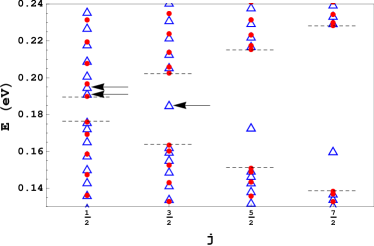
Figure 1: (Color online) Energy spectrum $E_{j,s,\pm}$ from numerical diagonalization of Eq. (2) for a cylindrical TI quantum dot with $R=20$ nm and $L=44$ nm. Open blue triangles correspond to the numerical results, while filled red circles show the analytical prediction in Eq. (35). Dashed lines indicate the surface gap for the respective angular momentum ($j$) mode in an infinitely long nanowire. The spin texture for the zero-momentum state with $j=1/2$ indicated by the lower left arrow is shown in Fig. 2. The spin texture for the next higher state (higher left arrow) is shown in Fig. 3. The example of a subgap state (for $j=3/2$, right arrow) is addressed in Fig. 4.

We now present the results of our numerical calculations. The discrete energy spectrum for a TI nanowire dot with $R=20$ nm and $L=44$ nm is shown in Fig. 1. The Kramers degeneracy results in an identical spectrum for $j\to-j$ but with reversed spin and parity ($\tau_{y}$) directions. We therefore show only the $j>0$ solutions in Fig. 1. Moreover, we focus on the topologically protected surface fermion modes inside the bulk gap $\Delta_{b}$.

There are several noteworthy points about Fig. 1. First, comparison with our analytical results, see Eq. (35) and Sec. III below, shows that most levels are approximately recovered from the bulk dispersion relation [Eq. (1)] by simply imposing the standard quantization condition $k_{n}=n\pi/L$ with $n\in\mathbb{N}$ on the longitudinal momentum $k$. However, here additional states corresponding to $n=0$ emerge. These zero-momentum states are absent for Schrödinger fermions in a box. Note that for each $j$, there is precisely one $n=0$ state for the conduction band and one for the valence band. Inspection of the density profiles for these states reveals almost homogeneous charge, spin, and parity densities as a function of the $z$ coordinate. Second, for $j>1/2$, we find a pair of nearly degenerate subgap states inside the surface gap $\Delta_{s}$. (The near-degeneracy is not visible in Fig. 1.) Such a subgap state is localized with equal occupation probability at both caps. Furthermore, electron-hole symmetry is broken under the Zhang model $H_{b}$, in contrast to the analytical model in Sec. III. This is the main reason for the existing discrepancies between Eq. (35) and the numerical results, see Fig. 1. In fact, we have also carried out additional numerical calculations for an electron-hole symmetric version of Eq. (2), where the corresponding results fit almost perfectly to the analytical results in Sec. III. In particular, all subgap states then disappear.

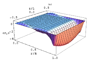
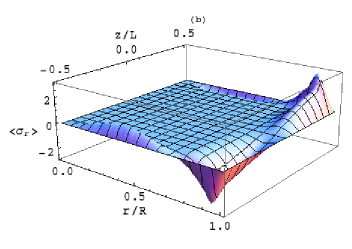
Figure 2: (Color online) Spin density components $\langle\sigma_{z}\rangle$ [(a)] and $\langle\sigma_{r}\rangle$ [(b)] in the $rz$ plane, for the zero-momentum state with $j=1/2$ indicated by the lower left arrow in Fig. 1.

Inspection of the spin densities, $\langle\sigma_{\alpha}\rangle(r,z)$, and parity densities, $\langle\tau_{\beta}\rangle(r,z)$, for a given eigenstate $(j,s,\pm)$ yields

$$\langle\sigma_{\phi}\rangle(r,z)=\langle\tau_{x}\rangle(r,z)=0,$$ (6)

i.e., spin is never oriented in the circumferential direction. In addition, there is now a finite radial spin component within the trunk region ($|z|<L/2$) and a finite $z$-component within the caps ($|z|=L/2$). Hence, in general, the spin direction for a surface state points out of the surface: spin-surface locking is broken in this geometry. This finding is in striking contrast to what happens in an infinite nanowireegger and for a sphere.dhlee Specifically, in the infinite cylinder case, the results corresponding to Fig. 2 show $\langle\sigma_{r}\rangle=0$ reflecting spin-surface locking.

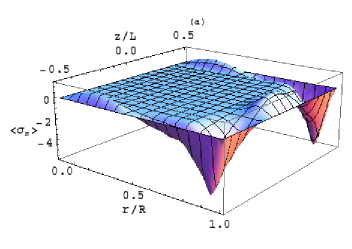
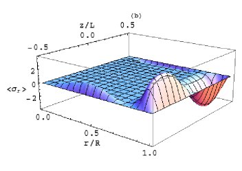
Figure 3: (Color online) Same as Fig. 2 but for the next higher energy level (upper left arrow in Fig. 1).

Figure 2 shows the spin density profile for the lowest-lying (“zero-momentum”) conduction band state with $j=1/2$, indicated by the lower left arrow in Fig. 1. We indeed find an almost homogeneous spin density profile along the trunk, where spin is mostly aligned along the (negative) $z$-direction, see Fig. 2(a). Also the charge density is practically homogeneous along the $z$-direction (data not shown). However, there is also a finite radial spin component breaking spin-surface locking, see Fig. 2(b). For the cap region, spin is mostly aligned along the radial direction, but again an out-of-plane component, now oriented along the $z$-axis, is clearly visible. For comparison, Fig. 3 shows the respective results for the next higher energy level (upper left arrow in Fig. 1). Again we observe that spin-surface locking is violated, while in the infinite cylinder case one finds $\langle\sigma_{r}=0\rangle$ (spin-surface locking).

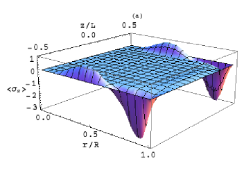
Figure 4: (Color online) Same as Fig. 2 but for the “subgap” state with $j=3/2$ indicated by the right arrow in Fig. 1.

For $j>1/2$, our numerical results include an almost degenerate pair of subgap states, where the degeneracy is on top of the Kramers degeneracy. The charge density is then localized with equal probability near each of the two cylinder caps. A typical example for the spin texture of such a subgap state is shown (for $j=3/2$) in Fig. 4. The out-of-plane spin part is identical on both caps, see Fig. 4(a), but the in-plane (radial) component shown in Fig. 4(b) has opposite direction.

Comparing our numerical results for parity, charge and spin densities, we find that for each eigenstate, they are linked by a set of general relations. In particular, for the (radially integrated) densities in the trunk region, we find

$$\langle\tau_{y}\rangle(z)\propto-\langle\sigma_{r}\rangle(z),\quad\langle\tau_{z}\rangle(z)\propto\langle\rho\rangle(z).$$ (7)

Note that in the infinite wire case,egger ; paco the parity structure is trivial in the sense that (for large $R$) the only non-zero component is $\langle\tau_{z}\rangle$, cf. Appendix A.

III Surface Dirac fermion theory

In this section, we analyze the finite-length nanowire geometry of Sec. II within a surface Dirac fermion theory, where we retain parity in the Hilbert space of the surface Hamiltonian. While this is not necessary for an infinite cylinderegger or for the flat 2D surface,zhang2 the discussion at the end of Sec. II.2 shows that this extension is important here.

III.1 Infinitely long wire and symmetries

We start with the parity-extended surface Dirac fermion Hamiltonian for an infinitely long nanowire,ashv0 ; egger

$$H_{D}=\left[v_{1}\sigma_{\phi}(-i\partial_{z})-\frac{v_{2}}{R}\sigma_{z}\hat{J}\right]{\cal T},$$ (8)

where the total angular momentum operator $\hat{J}$ has been defined in Eq. (4). ${\cal T}={\cal T}^{\dagger}$ acts in parity space and is determined below. We note that $H_{D}$ respects all symmetries present in $H_{b}$ [Eq. (2)]. Specifically, azimuthal symmetry implies $[H_{D},\hat{J}]=0$, and states are classified by half-integer $j$,

$$\psi(\phi,z)=e^{-i\sigma_{z}\phi/2}\sum_{j\in\mathbb{Z}+1/2}e^{ij\phi}\,\psi_{j}(z),$$ (9)

with the 1D spinor $\psi_{j}(z)$. Time-reversal symmetry implies $[H_{D},\Theta]=0$, with the time-reversal operator $\Theta=i\sigma_{y}\tau_{0}\,{\cal C}$, where ${\cal C}$ denotes complex conjugation. Finally, Eq. (8) exhibits inversion symmetry, $[H_{D},{\cal I}]=0$, with the inversion operatorfoot1

$${\cal I}=R_{z}R_{\phi}\sigma_{0}\tau_{z}.$$ (10)

Here, $R_{z}$ inverts the $z$ coordinate, $z\to-z$, and $R_{\phi}$ shifts $\phi\to\phi+\pi$. The parity structure in Eq. (10) follows from the results of Ref. zhang1, . Evidently, both time-reversal and inversion symmetry are only kept intact when choosing ${\cal T}\in\{\tau_{0},\tau_{z}\}$ in Eq. (8). We here set ${\cal T}=\tau_{z}$, as follows from the analytical derivation of Eq. (8) in Appendix A as well as from numerical calculations based on the Zhang model for the infinite nanowire case.egger

Using Eq. (9), we can now switch to a 1D representation for a given angular momentum ($j$) channel. For given energy $E$, the 1D spinor $\psi_{j}$ obeys the 1D Dirac equation $H^{(j)}\psi_{j}=E\psi_{j}$ withfoot2

$$H^{(j)}=\left(-iv_{1}\sigma_{y}\partial_{z}-\frac{jv_{2}}{R}\sigma_{z}\right)\tau_{z},$$ (11)

see also the derivation leading to Eq. (47) in Appendix A. Note that the representation of the Dirac matrices $\hat{\gamma}_{k}$ in Eq. (47) in terms of products of spin and parity matrices, see Eq. (11), is multi-valued and leads to a double counting of all surface states derived from Eq. (11). Nevertheless, it is technically convenient to proceed in this representation, since the double counting can be easily circumvented, see Sec. III.3.

The general solution to the 1D Dirac equation with Hamiltonian $H^{(j)}$ in Eq. (11) reads

$$\psi_{j}(z)=\left(\begin{array}[]{c}A_{1}\chi_{j}\\ -iA_{2}\sigma_{x}\chi_{j}\end{array}\right)e^{ikz}+\left(\begin{array}[]{c}B_{1}\chi_{j}^{\ast}\\ iB_{2}\sigma_{x}\chi_{j}^{\ast}\end{array}\right)e^{-ikz},$$ (12)

with arbitrary complex coefficients $(A_{1},A_{2},B_{1},B_{2})$. The spinors above are in parity space while $\chi_{j}$ acts in spin space,

$$\chi_{j}=\left(\begin{array}[]{c}\cos\gamma_{j}\\ i\sin\gamma_{j}\end{array}\right)\equiv\left(\begin{array}[]{c}\sqrt{\frac{1}{2}-\frac{jv_{2}}{2RE}}\\ i\ {\rm sgn}(E)\sqrt{\frac{1}{2}+\frac{jv_{2}}{2RE}}\end{array}\right).$$ (13)

In Eq. (12), the longitudinal momentum $k=k(E)$ follows from $v_{1}k=\sqrt{E^{2}-(jv_{2}/R)^{2}}$. Below we consider energies where $k$ is real and positive. For a description of the subgap states discussed in Sec. II.2, evanescent modes need to be studied instead. In the 1D representation, the inversion operator [Eq. (10)] becomes ${\cal I}\to\tilde{\cal I}$ with

$$\tilde{\cal I}=R_{z}\sigma_{z}\tau_{z}.$$ (14)

Since Eq. (11) stays invariant under inversion, $[H^{(j)},\tilde{\cal I}]=0$, the eigenfunctions (12) can be classified as inversion symmetric or antisymmetric ($\sigma=\pm$),

$$\tilde{\cal I}\psi_{j}^{(\sigma)}(z)=\sigma\psi_{j}^{(\sigma)}(z).$$ (15)

From Eqs. (12) and (15), after a short calculation, we can therefore infer relations between the coefficients for given inversion symmetry ($\sigma)$:

$$A_{1}=\sigma B_{1},\quad A_{2}=-\sigma B_{2}.$$

A general inversion-symmetric (antisymmetric) state thus takes the form

$$\psi_{j}^{(+)} = \left(\begin{array}[]{c}A_{1}\\ -iA_{2}\sigma_{x}\end{array}\right)\otimes\left(\begin{array}[]{c}\cos\gamma_{j}\ \cos(kz)\\ -\sin\gamma_{j}\ \sin(kz)\end{array}\right),$$ (20)

$$\psi_{j}^{(-)} = \left(\begin{array}[]{c}iA_{1}\\ A_{2}\sigma_{x}\end{array}\right)\otimes\left(\begin{array}[]{c}\cos\gamma_{j}\ \sin(kz)\\ \sin\gamma_{j}\ \cos(kz)\end{array}\right).$$ (25)

Both are parametrized by two complex numbers ($A_{1}$ and $A_{2}$), where the first (second) spinor refers to parity (spin) space.

Next let us take the local expectation value for the charge, spin, and parity operators in a given general eigenstate $\psi_{j}^{(\sigma)}$. First, with $\sin^{2}(\gamma_{-j})=\cos^{2}(\gamma_{j})$, the charge density is

$$\langle\rho\rangle(z)=\left(\left|A_{1}\right|^{2}+\left|A_{2}\right|^{2}\right)\left[\cos^{2}(\gamma_{\sigma j})\cos^{2}(kz)+\sin^{2}(\gamma_{\sigma j})\sin^{2}(kz)\right].$$ (26)

For the spin density, we obtain

$$\left(\begin{array}[]{c}\langle\sigma_{r}\rangle\\ \langle\sigma_{\phi}\rangle\\ \langle\sigma_{z}\rangle\end{array}\right)(z)=\sigma\left(\begin{array}[]{c}-\frac{1}{2}\left(|A_{1}|^{2}+|A_{2}|^{2}\right)\sin(2\gamma_{j})\sin(2kz)\\ 0\\ \left(|A_{1}|^{2}-|A_{2}|^{2}\right)\left[\cos^{2}(\gamma_{\sigma j})\cos^{2}(kz)-\sin^{2}(\gamma_{\sigma j})\sin^{2}(kz)\right]\end{array}\right).$$ (27)

Similarly, the parity density is obtained in the form

$$\left(\begin{array}[]{c}\langle\tau_{x}\rangle\\ \langle\tau_{y}\rangle\\ \langle\tau_{z}\rangle\end{array}\right)(z)=\left(\begin{array}[]{c}\sigma\,{\rm Im}(A_{1}A_{2}^{\ast})\sin(2\gamma_{j})\sin(2kz)\\ \sigma\,{\rm Re}(A_{1}A_{2}^{\ast})\sin(2\gamma_{j})\sin(2kz)\\ \left(|A_{1}|^{2}-|A_{2}|^{2}\right)\left[\cos^{2}(\gamma_{\sigma j})\cos^{2}(kz)+\sin^{2}(\gamma_{\sigma j})\sin^{2}(kz)\right]\end{array}\right).$$ (28)

At this stage, the above results hold for an arbitrary inversion-symmetric ($\sigma=+$) or antisymmetric ($\sigma=-$) state. Remarkably, the circumferentially oriented spin density $\langle\sigma_{\phi}\rangle$ always vanishes. This is in accordance with our numerical observations, see Eq. (6). The current density along the $z$ direction can be obtained from the local operatoregger

$$j_{z}=v_{1}\sigma_{\phi}\tau_{z},$$ (29)

and therefore vanishes identically for these states as well.footcur This result stays valid for arbitrary inversion-symmetric boundary conditions (which do not mix $\psi_{j}^{(\pm)}$ states).

In order to reach agreement with the numerical results in Sec. II.2, the coefficients $A_{1,2}$ should obey the three relations

$${\rm Im}(A_{1}A_{2}^{\ast})=0,\quad{\rm Re}(A_{1}A_{2}^{\ast})>0,\quad|A_{1}|\neq|A_{2}|.$$ (30)

Indeed, the first relation implies consistency with Eq. (6). The second relation ensures that $\langle\tau_{y}\rangle(z)\propto-\langle\sigma_{r}\rangle(z)$, see Eq. (7). The third relation is required to have non-vanishing spin-parity densities $\langle\sigma_{z}\rangle$ and $\langle\tau_{z}\rangle(z)$. Moreover, notice that then $\langle\tau_{z}\rangle(z)\propto\langle\rho\rangle(z)$, in accordance with Eq. (7).

III.2 Matching trunk and cap states

The coefficients $A_{1,2}$ in Eq. (20) as well as the energy spectrum and the corresponding eigenstates can now be obtained analytically by matching the trunk states, see Eq. (20) for $|z|<L/2$, with cap states at $z=\pm L/2$. Each cap is described by a surface Dirac Hamiltonian of the form

$$H_{\rm cap}=v_{2}\left[-i\left(\partial_{r}+\frac{1}{2r}\right)\sigma_{r}+\frac{\hat{J}}{r}\sigma_{\phi}\right]\tau_{x}.$$ (31)

The parity matrix $\tau_{x}$ is uniquely determined by imposing time-reversal and inversion symmetry, and also appears in Eq. (2). In the angular momentum (1D) representation, for given energy $E$, a cap state $\Psi_{j}^{(\sigma)}(r,z=\zeta L/2)$ [with $\zeta=\pm$ and inversion symmetry index $\sigma=\pm$] takes the general form (for $\sigma=\zeta=-$, this should be multiplied by $-1$)

$$\Psi_{j}^{(\sigma)}(r,\zeta L/2)=C_{\zeta}\left(\begin{array}[]{c}1\\ 1\end{array}\right)\otimes\xi_{j}(r)+C_{-\zeta}\left(\begin{array}[]{c}1\\ -1\end{array}\right)\otimes\xi_{j}^{\ast}(r)$$ (32)

with complex coefficients $C_{\pm}$ and the spin spinor

$$\xi_{j}(r)=\left(\begin{array}[]{c}J_{j-1/2}(|E|r/v_{2})\\ i\,{\rm sgn}(E)J_{j+1/2}(|E|r/v_{2})\end{array}\right).$$ (33)

The other spinors in Eq. (32) are in parity space.

Matching the trunk states [Eq. (20)] and the cap states [Eq. (32)] for given $j$ and $\sigma$ by continuity at $z=\pm L/2$ and $r=R$, we obtain four linear equations for the four coefficients $(A_{1},A_{2},C_{+},C_{-})$. A nontrivial solution follows when the corresponding determinant vanishes, yielding the condition ($u=|E|R/v_{2}$)

$$\left(J^{2}_{j-1/2}(u)+J^{2}_{j+1/2}(u)\right)\sin(2\gamma_{j})\sin(kL)=0.$$ (34)

For real-valued $k\geq 0$, this equation can only be satisfied when $\sin(kL)=0$. This implies the standard longitudinal momentum quantization condition $k_{n}(E)=n\pi/L$ with $n\in\mathbb{N}_{0}$. The corresponding eigenenergies then follow from the bulk dispersion relation in Eq. (1),

$$E_{j,n,\pm}=\pm\sqrt{(\pi nv_{1}/L)^{2}+\left(jv_{2}/R\right)^{2}}.$$ (35)

For a given level, the wave function amplitudes $A_{1,2}$ and $C_{\pm}$ then satisfy three conditions plus the overall normalization constraint. With $p=\sigma(-)^{n}=\pm$ and the above definition of $u$, we have $C_{+}=pC_{-}$ and the relation

$$J_{j+p/2}(u)A_{1}+p\ {\rm sgn}(E)\ J_{j-p/2}(u)A_{2}=0.$$ (36)

Moreover, for $p=+$ the third condition reads

$$\cos(\gamma_{j})A_{1}-2(-i)^{n}J_{j-1/2}(u)C_{+}=0,$$ (37)

while for $p=-$ this instead becomes

$$\sin(\gamma_{j})A_{1}-2(-i)^{n}\ {\rm sgn}(E)\ J_{j+1/2}(u)C_{+}=0.$$

These relations determine all possible wavefunctions for the closed cylinder surface.

Of course, since we considered only solutions of Eq. (34) with real $k$, subgap states were not captured. However, within the linear-in-${\bm{k}}$ approximation underlying the approach here, we find that there are no subgap states at all, i.e., the corresponding matching problem with evanescent trunk modes does not permit a nontrivial solution. The numerical approach of Sec. II also indicates that in order to obtain subgap states, it is necessary to include higher-order terms (in ${\bm{k}}$) breaking electron-hole symmetry in the Hamiltonian.

III.3 Spectrum and eigenstates of the dot

Using the above explicit solution for the wavefunction of the complete cylinder, we obtain the coordinate dependence of all densities of interest. We here describe the results for the trunk region only. First of all, we recover

$$\langle\sigma_{\phi}\rangle=\langle\tau_{x}\rangle=0,$$

see Eq. (6). Moreover, the relations

$$\langle\tau_{y}\rangle\propto-\langle\sigma_{r}\rangle,\quad\langle\tau_{z}\rangle\propto\langle\rho\rangle$$

are also reproduced, see Eq. (7). Specifically, the dot eigenstates have the energy $E\equiv E_{j,n,\pm}$ specified in Eq. (35). We show below that these energies are not degenerate, i.e., only one specific inversion parity $\sigma$ given by

$$\sigma\equiv\sigma_{j,n,\pm}=\mp(-1)^{n}{\rm sgn}(j)$$ (38)

will be physically realized. With $k\equiv\pi n/L\geq 0$, we find for the charge and spin densities ($u=|E|R/v_{2}$)

$$\langle\rho\rangle(z) \propto 1-{\rm sgn}(E)\frac{j\sigma}{u}\cos(2kz),$$

$$\langle\sigma_{r}\rangle(z) \propto \sqrt{1-j^{2}/u^{2}}\ \sin(2kz),$$ (39)

$$\langle\sigma_{z}\rangle(z) \propto \cos(2kz)-\frac{j\sigma}{u}{\rm sgn}(E).$$

These results are in good agreement with the numerical results for the spin texture obtained for the Zhang model in Sec. II. In particular, they show explicitly that spin-surface locking is broken.

Interestingly, for each total angular momentum $j$, there are two zero-momentum states corresponding to conduction and valence band, respectively. Their inversion symmetry properties are determined by

$$\sigma=-{\rm sgn}(jE_{j,n=0,\pm}),$$ (40)

since for states with the opposite value of $\sigma$, all densities in Eq. (39) vanish. For the physically allowed $k=0$ state with $\sigma$ in Eq. (40), from Eq. (39) we instead find spatially uniform densities $\langle\rho\rangle(z)$, $\langle\tau_{z}\rangle(z)$, and $\langle\sigma_{z}\rangle(z)$, while all remaining spin or parity density components vanish.

We now compare the densities in Eq. (39) to the numerical results in Sec. II, and also address the double counting problem mentioned in Sec. III.1. Eq. (36) shows that indeed ${\rm Im}(A_{1}A_{2}^{\ast})=0$, in accordance with our numerical results in Sec. II.2, see Eq. (30). Also the relation $|A_{1}|\neq|A_{2}|$ in Eq. (30) is evidently satisfied. However, not all the states can be realized physically, as is clear by comparing to the condition ${\rm Re}(A_{1}A_{2}^{\ast})>0$ in Eq. (30) found numerically in Sec. II. In order to understand this restriction, we note that the operator $\Xi=\sigma_{z}\tau_{z}$ commutes both with the cap Hamiltonian [Eq. (31)] and with the inversion operator $\tilde{\cal I}$ [Eq. (14)]. This implies by continuity that trunk states [Eq. (20)] at the end points ($z=\zeta L/2$ with $\zeta=\pm$) are eigenstates of $\Xi$ as well,

$$\Xi\psi_{j,n}^{(\sigma)}(\zeta L/2)=p\psi_{j,n}^{(\sigma)}(\zeta L/2),$$

where the eigenvalues $p=\sigma(-1)^{n}$ follow from Eq. (20) and the definition of $\Xi$. For $n=0$, however, Eq. (40) implies that only the eigenvalue $p=-{\rm sgn}(jE_{j,0,\pm})$ is physically realized. By continuity, this value must also apply for the full Hilbert space of conduction or valence surface bands. We therefore obtain the “selection rule” in Eq. (38) restricting the Hilbert space of allowed states. This explains the condition ${\rm Re}(A_{1}A_{2}^{\ast})>0$ and resolves the double-counting problem. We mention in passing that the latter problem is automatically avoided when retaining terms of order ${\bm{k}}^{2}$ in the Hamiltonian, where the spin-parity eigenstates with $p=\pm$ have different energy. In the Dirac theory, this implies a “spontaneously broken symmetry” encoded by Eq. (38).

III.4 Effective boundary conditions

It is also possible to derive the results in Sec. III.3 without explicit construction of the cap states. To that end, let us briefly consider a class of general boundary conditions at the cylinder ends, $z=\zeta L/2$ with $\zeta=\pm$, by imposing the local gauge constraints

$$\psi(\phi,\zeta L/2)=\Lambda_{\zeta}\,\psi(\phi,\zeta L/2),$$ (41)

where $\Lambda_{\zeta}=\Lambda_{\zeta}^{-1}=\Lambda_{\zeta}^{\dagger}$. The spin-parity structure of $\Lambda_{\zeta}$ can be determined by requiring time-reversal invariance, $[\Lambda_{\zeta},\Theta]=0$, and invariance under inversion, $[\Lambda_{\zeta},{\cal I}]=0$. In addition, we require the boundary operator to commute with $H_{D}$, which is a natural assumption for closed surfaces. As a result, with arbitrary angles $\eta_{\pm}$, we find

$$\Lambda_{\zeta}=\sin(\eta_{\zeta})\sigma_{0}\tau_{z}+\cos(\eta_{\zeta})\sigma_{r}\tau_{y}.$$

Passing to the 1D representation, i.e., for given half-integer $j$, these constraints read

$$\psi_{j}(\zeta L/2) = \tilde{\Lambda}_{\zeta}\psi_{j}(\zeta L/2),$$ (42)

$$\tilde{\Lambda}_{\zeta} = \sin(\eta_{\zeta})\sigma_{0}\tau_{z}+\cos(\eta_{\zeta})\sigma_{x}\tau_{y}.$$

Applying the inversion operator $\tilde{\cal I}$, see Eq. (14), to the boundary condition (42), we find $\tilde{\Lambda}_{+}=\tilde{\Lambda}_{-}$ and hence $\eta_{\pm}\equiv\eta$. Only then will inversion symmetry be preserved for the confined states. The parameter $\eta$ (with $0\leq\eta<\pi$) cannot be fixed by symmetry considerations alone but depends on the physical boundary condition imposed at the ends, i.e., the boundary matrix $\tilde{\Lambda}$ effectively encodes the matching of trunk states with cap states. Contrary to the commonly employed boundary conditions,falko ; akhmerov the operator $\tilde{\Lambda}$ commutes with the current operator $j_{z}$, see Eq. (29), while the anticommutator is always nonzero. Since the boundary conditions are invariant with respect to inversion, they do not mix the states (20) with opposite inversion parity $\sigma$. Using the boundary condition (42), some algebra yields for both solutions and for arbitrary energy $E$ the condition

$$A_{1}+\frac{\cos\eta}{1-\sin\eta}A_{2}=0.$$ (43)

Comparing this to Eq. (36), the energy-dependent angle $\eta$ can be explicitly related to the above wavefunction matching procedure, and the subsequent results in Sec. III.3 can be obtained under a purely 1D description of the trunk states alone.

IV Microscopic tight-binding approach

A simple microscopic model for a strong TI was previously proposed by Fu, Kane, and Mele.fu-kane-mele-07 The model consists of a single-band tight-binding model on a diamond lattice and includes spin-orbit couplings. With lattice fermion operators $c_{i}$ (spin is kept implicit), this Hamiltonian has the form

$$H_{\rm tb}=\sum_{\langle i,j\rangle}t_{ij}c_{i}^{\dagger}c_{j}+\frac{4i\lambda_{\rm so}}{a^{2}}\sum_{\langle\langle i,j\rangle\rangle}c_{i}^{\dagger}\left({\bm{\sigma}}\cdot\left[{\bm{d}}_{ij}^{1}\times{\bm{d}}_{ij}^{2}\right]\right)c_{j},$$ (44)

where $a$ is the cubic lattice constant, $t_{ij}$ are hopping parameters connecting nearest neighbors, and the last term describes spin-orbit coupling of strength $\lambda_{\rm so}$ through a second-neighbor hopping between sites $i,j$, which depends on the two nearest-neighbor vectors ${\bm{d}}^{1,2}$ connecting those two sites. In order to generate a full gap in the bulk spectrum, a distortion $t_{ij}\rightarrow t+\delta t$ is introduced for ${\bm{d}}_{ij}$ along the (111) direction.fu-kane-mele-07

To define the nanowire, we proceed as in Ref. egger, by selecting the growth direction $\hat{e}_{z}$ along the (111) axis and keeping all sites within a given radius $R$. The unit cell of the infinite nanowire thus defined contains six planes of sites corresponding to the three stackings of the two fcc sublattices of the diamond lattice, and has the period $d_{\rm cell}=\sqrt{3}a$. Although this model is not completely equivalent to the one of Eq. (2), quantitatively similar behavior of the surface gap $\Delta_{s}$ as a function of $R$ has been obtainedegger by setting $a=2.8$ nm and $-2t+\delta t=M_{0}$. The finite dot geometry is then defined by setting the length of the nanowire along the (111) direction to a given value $L$. To maintain the aspect ratio of the cylindrical dot studied numerically in Sec. II, we set $R=3a$ and $L=4\sqrt{3}a$. This corresponds to a cluster of 1592 sites, which is a small enough size to keep a reasonable computational cost of the calculations while still allowing for a meaningful comparison of the spin texture with the results of Secs. II and III.

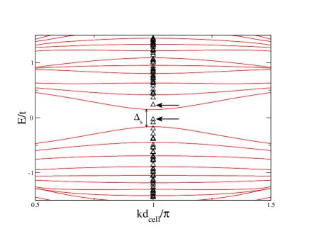
Figure 5: (Color online) Band structure of the infinite TI nanowire (red solid curves) and energy levels (denoted by open black triangles) of a finite dot. These results follow from the tight-binding model [Eq. (44)] with wire axis along the (111) direction. The dot length is set to $L=4\sqrt{3}a$, and the radius is $R=3a$. The arrows indicate the two levels whose spin texture is analyzed in Figs. 6 and 7, respectively.

The band structure of the infinite nanowire and the energy levels in the finite dot geometry are shown in Fig. 5, where we again focus on states energetically inside the bulk gap. As expected, both the bands of the infinite wire and all dot levels are twofold Kramers degenerate. For the chosen parameter set, we find two subgap states appearing inside the surface gap $\Delta_{s}$. (Since there is no full rotational symmetry anymore, we cannot classify states by $j$ here.)

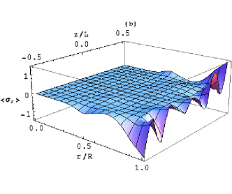
Figure 6: (Color online) Spin texture in the $rz$ plane obtained from the tight-binding model [Eq. (44)]. The spin densities $\langle\sigma_{z}\rangle$ [(a)] and $\langle\sigma_{r}\rangle$ [(b)] are shown for the subgap state indicated by the lower arrow in Fig. 5.

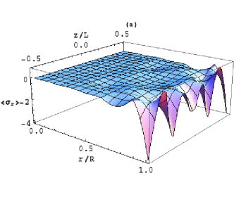
Figure 7: (Color online) Same as Fig. 6 but for the state indicated by the higher arrow in Fig. 5.

To get an idea of the spin texture of the dot states, we now focus on the two states indicated by arrows in Fig. 5. The lower arrow corresponds to a subgap state, and the second one refers to the lowest-lying state within the conduction band of the infinite wire. The corresponding spin densities are shown in Figs. 6 and 7. As in the effective low-energy theory and the surface Dirac fermion description, we again observe $\langle\sigma_{\phi}\rangle=0$, and therefore only $\langle\sigma_{z}\rangle$ and $\langle\sigma_{r}\rangle$ are shown. Note that in the infinite wire case, one would instead find $\langle\sigma_{r}\rangle=0$ consistent with spin-surface locking.egger

The subgap states have a charge density mostly localized near the caps of the cylindrical dot, again with out-of-plane (in-plane) spin components that are identical (oppositely directed) on both sides, reproducing the results of Secs. II and III. However, unlike the continuous model, the tight-binding model predicts a spin texture with a superimposed atomic-scale oscillation. This oscillation stems from the finite $k=\pi/d_{\rm cell}$ value at the Dirac point in this model.

On the other hand, for the lowest-lying state within the conduction band, corresponding to the “zero-momentum” state in Secs. II and III, Figure 7 shows that the density is largest along the cylinder trunk. The spin is predominantly oriented along the negative $z$-direction, but with a finite oscillatory component in the radial direction that breaks spin-surface locking.

To conclude, even though the results of the tight-binding model are not fully equivalent to the ones in Secs. II and III, we find that the main properties of the subgap and lowest conduction band states are reproduced.

V Conclusions

In this paper we have studied the band structure of a quantum dot made of a strong topological insulator using three different approaches, namely the low-energy theory of Zhang et al.,zhang1 ; zhang2 an effective surface Dirac fermion theory, and numerical calculations for a tight-binding model on a diamond lattice with strong spin-orbit couplings. The considered geometry, with flat caps terminating a finite-length cylindrical nanowire, is characterized by sharp edges where the cylinder trunk and caps meet. Such edges are also present in typical “mesoscopic” TI devices studied experimentally.peng ; cha ; zuev ; tang All three approaches show that spin-surface locking is generally violated due to presence of these edges. As also found in a recent ab initio study,moon a finite reflection probability for Dirac fermions in each part results when two surfaces are patched together. In our case, we have a Fabry-Perot-like setup where standing waves can build up. The resulting spin density then exhibits spatial oscillations reminiscent of a spin density wave state. The spin direction of the oscillatory parts points out of the surface while non-oscillatory spin density contributions stay locked to the surface.

The spectrum of such a quantum dot shows several surprising features. First, when starting from the band structure of the infinitely long wire [Eq. (1)], imposing the usual longitudinal quantization condition, $k_{n}=n\pi/L$, here allows for a nontrivial eigenstate with $k=n=0$. In such a zero-momentum state the charge and spin densities along the trunk are basically homogeneous. Second, albeit the surface bands of an infinite nanowire exhibit a gap, the finite-length nanowire dot has subgap states when electron-hole symmetry is broken. The wavefunction of such a subgap state is localized on both caps simultaneously. The obtained energy spectrum and corresponding spin textures are important ingredients for a theory of mesoscopic transport through TI dots. In general, we also expect Coulomb interactions to be relevant, in particular charging effects should be visible. We plan to address these questions in the future. Moreover, extensions of the theory to include an applied magnetic field, where the typically large and anisotropic Landé factorzhang2 implies that the Zeeman field is crucial, are also left for future work.

Appendix A Surface Hamiltonian for infinite nanowire

	$\tau_{0}$	$\tau_{x}$	$\tau_{y}$	$\tau_{z}$
$\sigma_{0}$	$\hat{\gamma}_{0}$	$0$	$\hat{\gamma}_{x}$	$0$
$\sigma_{x}$	$-\hat{\gamma}_{x}$	$0$	$-\hat{\gamma}_{0}$	$0$
$\sigma_{y}$	$0$	$\hat{\gamma}_{z}$	$0$	$\hat{\gamma}_{y}$
$\sigma_{z}$	$0$	$\hat{\gamma}_{y}$	$0$	$-\hat{\gamma}_{z}$

Table 2: Representation of spin-parity matrices in terms of Pauli matrices $\hat{\gamma}_{i}$ acting in surface-state subspace.

Here we analytically derive Eq. (8) for an infinite nanowire using the gap-inversion model of Ref. paco, . Our starting point is Eq. (2) to linear order in ${\bm{k}}$ (we put $C_{0}=0$ here),

$$H_{b}=M\sigma_{0}\tau_{z}+\left[v_{1}k\sigma_{z}+v_{2}(k_{x}\sigma_{x}+k_{y}\sigma_{y})\right]\tau_{x}.$$ (45)

Following Ref. paco, , we assume that the gap parameter changes sign at $r=R$, i.e., $M(r)=M_{0}\ {\rm sgn}(R-r)$ with $M_{0}>0$. For $r<R$ ($r>R$), the material is then in the topologically nontrivial (trivial) phase. In the 1D representation, for given $j$ and $k$, solutions to the Dirac equation take the form $e^{ikz}\ e^{-i\sigma_{z}\phi/2}\sum_{j}e^{ij\phi}\,\psi_{j}(r)$, with the 1D radial Dirac equation

$$\left(H_{0}^{(j)}+v_{1}k\sigma_{z}\tau_{x}\right)\psi_{j}=E\psi_{j}.$$

Here $k=0$ corresponds to

$$H_{0}^{(j)}=M(r)\sigma_{0}\tau_{z}+v_{2}\left[-i\left(\partial_{r}+\frac{1}{2r}\right)\sigma_{x}+\frac{j}{r}\sigma_{y}\right]\tau_{x}.$$

For $k=0$, there are two solutions

$$\psi_{j}^{(s=\pm)}(r)=\left(\begin{array}[]{c}is\cos\gamma\\ -{\rm sgn}(M)\sin\gamma\end{array}\right)\otimes\left(\begin{array}[]{c}I_{j-1/2}(\kappa r)\\ -sI_{j+1/2}(\kappa r)\end{array}\right),$$

where the first (second) spinor refers to parity (spin) space, $\sin\gamma=\sqrt{\frac{1}{2}-\frac{E}{2M}}$, $\cos\gamma=\sqrt{\frac{1}{2}+\frac{E}{2M}}$, and $v_{2}\kappa=\sqrt{M_{0}^{2}-E^{2}}.$ For $r>R$, we have to replace $I_{j-1/2}\to K_{j-1/2}$ and $I_{j+1/2}\to-K_{j+1/2}$ in the spin part, where $I_{\nu}$ and $K_{\nu}$ are modified Bessel functions. The general solution is then given by

$$\psi_{j}(r)=\left\{\begin{array}[]{cc}\alpha_{1}\psi_{j}^{(+)}(r)+\beta_{1}\psi_{j}^{(-)}(r),&r<R,\\ \alpha_{2}\psi_{j}^{(+)}(r)+\beta_{2}\psi_{j}^{(-)}(r),&r>R,\end{array}\right.$$ (46)

where the coefficients $\alpha_{1,2}$ and $\beta_{1,2}$ are obtained by requiring continuity of the wave function at $r=R$. This results in a linear system of equations for the coefficients, which has a nontrivial solution under the condition

$$\left(\cos^{2}(\gamma)I_{j-1/2}K_{j+1/2}-\sin^{2}(\gamma)I_{j+1/2}K_{j-1/2}\right)$$

$$\times \left(\sin^{2}(\gamma)I_{j-1/2}K_{j+1/2}-\cos^{2}(\gamma)I_{j+1/2}K_{j-1/2}\right)=0,$$

where all Bessel functions have the argument $\kappa R$ and $\gamma$ is evaluated for $M=M_{0}$. Assuming $\kappa R\gg 1$ and using the asymptotic form of the Bessel functions, we find $\cos(2\gamma)\simeq\pm j/(\kappa R)$ and thus $E_{j,\pm}(k=0)=\pm jv_{2}/R$. The corresponding $k=0$ wavefunctions, $\psi_{j,\pm}(r)$, are given by Eq. (46) with $\beta_{1}=\pm\alpha_{1}$, $\beta_{2}=\pm\alpha_{2}$, and

$$\alpha_{1}=\sqrt{\frac{\pi}{2}}\kappa e^{-\kappa R},\quad\alpha_{2}=\mp\frac{\kappa}{\sqrt{2\pi}}e^{\kappa R}.$$

For small $k\neq 0$, the effective surface Hamiltonian, Eq. (8), is obtained by projecting Eq. (45) onto the subspace spanned by the above $k=0$ states. We thereby find

$$H^{(j)}=\frac{jv_{2}}{R}\hat{\gamma}_{z}+v_{1}k\hat{\gamma}_{y},$$ (47)

where the $\hat{\gamma}_{i}$ are Pauli matrices in the zero-momentum subspace. In this way, all combinations of spin-parity matrices, $\sigma_{i}\tau_{j}$, can be represented in the truncated basis. For $\kappa R\gg 1$, we obtain the results in Table 2. Of course, this representation is not single-valued, i.e., there is no one-to-one correspondence between the $\sigma_{i}\tau_{j}$ and the $\hat{\gamma}_{k}$ matrices. In particular, the spin operators $\sigma_{y,z}$ and the parity operator $\tau_{z}$ are entangled, since $\sigma_{y,z}\tau_{0}=0$ and $\sigma_{0}\tau_{z}=0$. Taking $\hat{\gamma}_{y}=\sigma_{y}\tau_{z}$ and $\hat{\gamma}_{z}=-\sigma_{z}\tau_{z}$, cf. the last column of Table 2, one gets the surface Hamiltonian quoted in the main text, see Eq. (11). Because this representation is multi-valued, the replacement of $\hat{\gamma}_{y,z}$ by products of spin and parity matrices causes a double-counting of states if used naively. This double-counting problem is, however, not severe and can be circumvented, as we discuss in Sec. III.3 in the main text.

References

- (1) M.Z. Hasan and C.L. Kane, Rev. Mod. Phys. 82, 3045 (2010).
- (2) X.-L. Qi and S.-C. Zhang, Physics Today 63, 33 (2010).
- (3) M.Z. Hasan and J.E. Moore, arXiv:1011.5462.
- (4) Y. Xia, D. Qian, D. Hsieh, L. Wray, A. Pal, H. Lin, A. Bansil, D. Grauer, Y.S. Hor, R.J. Cava, and M.Z. Hasan, Nature Physics 5, 398 (2009).
- (5) D.X. Qu, Y.S. Hor, J. Xiong, R.J. Cava, and N.P. Ong, Science 329, 821 (2010).
- (6) J.G. Checkelsky, Y.S. Hor, R.J. Cava, and N.P. Ong, arXiv:1003.3883
- (7) H. Peng, K. Lai, D. Kong, S. Meister, Y. Chen, X.L. Qi, S.C. Zhang, Z.X. Shen, and Y. Cui, Nature Mat. 9, 225 (2010).
- (8) J.J. Cha, J.R. Williams, D. Kong, S. Meister, H. Peng, A.J. Bestwick, P. Gallagher, D. Goldhaber-Gordon, and Y. Cui, Nano Lett. 10, 1076 (2010).
- (9) Y.M. Zuev, J.S. Lee, C. Galloy, H. Park, and P. Kim, Nano Lett. 10, 1076 (2010).
- (10) H. Tang, D. Liang, R.L.J. Qiu, and X.P.A. Gao, arXiv:1101.2152.
- (11) Y. Zhang, Y. Ran, and A. Vishwanath, Phys. Rev. B 79, 245331 (2009).
- (12) R. Egger, A. Zazunov, and A. Levy Yeyati, Phys. Rev. Lett. 105, 136403 (2010).
- (13) J.H. Bardarson, P.W. Brouwer, and J.E. Moore, Phys. Rev. Lett. 105, 156803 (2010).
- (14) Y. Zhang and A. Vishwanath, Phys. Rev. Lett. 105, 206601 (2010).
- (15) J. Nygard, D.H. Cobden, and P.E. Lindelof, Nature 408, 342 (2000).
- (16) H.W.C. Postma, T. Teepen, Z. Yao, M. Grifoni, and C. Dekker, Science 293, 76 (2001).
- (17) D.H. Lee, Phys. Rev. Lett. 103, 196804 (2009).
- (18) V. Parente, P. Lucignano, P. Vitale, A. Tagliacozzo, and F. Guinea, arXiv:1011.0565.
- (19) We note that a theory for quantum dots based on the 2D semiconductors HgTe and HgS (which may have topological phases) was recently put forward by N. Malkova and G.W. Bryant, Phys. Rev. B 82, 155314 (2010).
- (20) H. Zhang, C.X. Liu, X.L. Qi, X. Dai, Z. Fang, and S.C. Zhang, Nature Phys. 5, 438 (2009).
- (21) C.X. Liu, X.L. Qi, H.J. Zhang, X. Dai, Z. Fang, and S.C. Zhang, Phys. Rev. B 82, 045122 (2010).
- (22) L. Fu, Phys. Rev. Lett. 103, 266801 (2009).
- (23) O.V. Yazyev, J.E. Moore, and S.G. Louie, Phys. Rev. Lett. 105, 266806 (2010).
- (24) S. Souma et al., arXiv:1101.3421.
- (25) S.Y. Xu et al., arXiv:1101.3985.
- (26) A.A. Burkov and D.G. Hawthorn, Phys. Rev. Lett. 105, 066802 (2010).
- (27) M. König, H. Buhmann, L.W. Molenkamp, T. Hughes, C.X. Liu, X.L. Qi, and S.C. Zhang, J. Phys. Soc. Jpn. 77, 031007 (2008).
- (28) Under inversion, we have , while .
- (29) In the 1D representation (9), the cylindrical Pauli matrices in Eq. (3) are replaced by .
- (30) For current-carrying states, one has to impose boundary conditions breaking the inversion symmetry.
- (31) E. McCann and V.I. Fal’ko, J. Phys.: Cond. Matt. 16, 2371 (2004).
- (32) A.R. Akhmerov and C.W.J. Beenakker, Phys. Rev. B 77, 085423 (2008).
- (33) L. Fu, C.L. Kane, and E.J. Mele, Phys. Rev. Lett. 98, 106803 (2007).
- (34) C.Y. Moon, J. Han, H. Lee, and H.J. Choi, arXiv:1101.0210.