Selection models with monotone
weight functions in meta analysis

Abstract

Publication bias, the fact that studies identified for inclusion in a meta analysis do not represent all studies on the topic of interest, is commonly recognized as a threat to the validity of the results of a meta analysis. One way to explicitly model publication bias is via selection models or weighted probability distributions. We adopt the nonparametric approach initially introduced by Dear and Begg (1992) but impose that the weight function $w$ is monotonely non-increasing as a function of the $p$-value. Since in meta analysis one typically only has few studies or “observations”, regularization of the estimation problem seems sensible. In addition, virtually all parametric weight functions proposed so far in the literature are in fact decreasing. We discuss how to estimate a decreasing weight function in the above model and illustrate the new methodology on two well-known examples. The new approach potentially offers more insight in the selection process than other methods and is more flexible than parametric approaches. Some basic properties of the log-likelihood function and computation of a $p$-value quantifying the evidence against the null hypothesis of a constant weight function are indicated. In addition, we provide an approximate selection bias adjusted profile likelihood confidence interval for the treatment effect. The corresponding software and the datasets used to illustrate it are provided as the R package selectMeta (Rufibach, 2011). This enables full reproducibility of the results in this paper.

Keywords. global constrained optimization, meta analysis, monotone non-increasing, selection bias

1 Introduction

Meta analysis has become a widely used technique for synthesizing evidence from different studies, see e.g. Sutton and Higgins (2008) for an overview over recent developments. Publication bias, i.e. the fact that studies identified for inclusion in a meta analysis, do not represent all studies on the topic of interest, is commonly recognized as a threat to the validity of the results of a meta analysis. Overviews how to prevent, assess, and adjust for publication bias are provided in Sutton et al. (2000), Macaskill et al. (2001), or Rothstein et al. (2005).

Numerous tools to detect publication bias in meta analysis have been developed, see Rothstein et al. (2005, Chapters 5-11) for an excellent overview of the current state-of-the-art.

If one seeks to assess selection bias one typically requires some model for the sampling behavior of the observed effect sizes that explicitly incorporates the selection process (Hedges and Vevea, 2005). It is hence useful to distinguish two parts of such a model: the effect size part and the selection part. The former specifies what the distribution of the effect sizes would be if there were no selection whereas the latter explicitly models how the effect size distribution is modified by the selection process. Two different classes of explicit selection models have been proposed so far for meta analysis (Hedges and Vevea, 2005). The first class depends on the effect size estimate, such as relative risk or odds ratio, and the corresponding standard error separately, see Copas (1999), Copas and Shi (2000), Copas and Shi (2001), and the implementation in the R package copas (Carpenter et al., 2009). This type of model is typically denoted “Copas selection model”. In the second class the weight is assumed to depend on the effect size only via the $p$-value associated with the study, see Hedges (1984), Iyengar and Greenhouse (1988), Hedges (1992), Dear and Begg (1992), Hedges and Vevea (2005, p. 149) or Copas and Malley (2008) for a test on selection bias that is robust against any form of selection function. The rationale to make the weight function depending on $p$-values, or equivalently on the standardized effect size, exclusively is that often, decisions about conclusiveness of medical research results are based on statistical significance (only).

More specifically, following the development in Hedges and Vevea (2005), let $Y^{*}$ be a random variable with density $f(y|\theta,\sigma)$ representing the effect estimate before selection, typically assumed to follow a normal distribution. Denoting the weight function by $w(y)$, the weighted density of the observed effect estimate $Y$ is then given by

$$g(y|\theta,\sigma) = \frac{f(y|\theta,\sigma)w(y)}{\int f(y|\theta,\sigma)w(y)\,\mathrm{d}y}.$$

Whenever the weight function $w$ is not constant, the sampling distribution of the observed effect size $Y$ differs from that of the unselected effect size $Y^{*}$ and this difference, i.e. the shape of $w$, is a way of describing selection bias.

Now, if larger values of $Y^{*}$ are more likely to be observed than smaller values, $w(y)$ is a monotone non-decreasing function of the effect size $y$. Considering $w$ on the scale of $p$-values this implies that $w(p)$ as a function of the $p$-value is non-increasing, meaning that smaller $p$-values are more likely to be observed than larger $p$-values. In this paper we propose a non-increasing estimate $\hat{w}(p)$ in the nonparametric normal model introduced by Dear and Begg (1992). Besides being a plausible assumption as elaborated above, nonparametrically estimating the weight function $w(p)$ and imposing a monotonicity constraint has further advantages:

• All parametric weight functions proposed in the literature are in fact non-increasing, see Section 3 for a brief discussion.

• Typically, the number of studies that enter a meta analysis is small to moderate. For this reason, additional regularization, such as monotonicity, and therewith constraining the parameter space, may lead to more realistic but still flexible estimates of the weight function compared to the purely nonparametric approach by Hedges (1992) and Dear and Begg (1992), but without forcing a purely parametric model. This makes our approach less prone to misspecification. See also the comment in Hedges (1988, p. 118).

• Restricting the parameter space, or shape of the function as in our case, typically yields estimates with better performance, e.g. measured in terms of mean squared error, if in fact the function to be estimated has the assumed shape, see e.g. Kelly (1989, p. 937).

• In contrary to e.g. kernel estimators or the penalized monotone estimator of Sun and Woodroofe (1997) the estimator $(\boldsymbol{\hat{w}},\hat{\theta},\hat{\sigma}^{2})$ defined below does not necessitate the choice of a smoothing or penalty tradeoff parameter (or a prior) and is therefore fully automatic.

• Weight functions are primarily proposed as an exploratory and informal means to assess the degree of publication bias which may be present, see Dear and Begg (1992, p. 240) or Sutton et al. (2000, p. 431). Specifically, if there is no selection effect at work, the former authors claim that the graphs of their estimated unconstrained weight function “provide visual confirmation of the lack of bias, demonstrating a seemingly random configuration of estimated weights.” However, it is not without difficulty to identify the model without biased selection from the estimated weight functions in sub-figures (a), (b), (c) of Dear and Begg (1992, Figure 2). As reveal our examples in Section 7, the monotonicity assumption typically yields more insight in the actual selection process.

In Section 2 we derive the log-likelihood function in our nonparametric model and provide some properties of it whereas in Section 3 we discuss different approaches to setup selection models and choose sensible selection functions. Section 4 elaborates on the computation of our proposed estimate. A discussion of statistical inference for the effect $\theta$ and the random effects variance component $\sigma^{2}$ are provided in Section 5. Specifically, in this section we sketch derivation of a profile likelihood confidence interval for the selection bias adjusted treatment effect $\theta$. A way to quantify evidence against the null hypothesis of no selection is described in Section 6. The paper is concluded with the analysis of two well-known examples and a discussion of the software package selectMeta (Rufibach, 2011) that enables full reproducibility of the results presented in this paper.

2 The log-likelihood function and its properties

To fix ideas, assume that there are $n$ independent studies with normally distributed observed treatment effects $Y_{i}$, $i=1,\ldots,n$ where $\mathop{\rm I\!E}\nolimits(Y_{i})=\theta$ and $\mathop{\rm Var}\nolimits(Y_{i})=\eta_{i}^{2}=u_{i}^{2}+\sigma^{2}$. Here, $u_{i}^{2}$ is the known sampling variance in the $i$-th study (largely determined by the sample size in the $i$-th study and therefore considered known) and $\sigma^{2}$ is a random effects component of variance representing the heterogeneity in the population. Typically, it is assumed that the effects follow a normal distribution, i.e. $Y_{i}\sim N(\theta,\eta_{i}^{2})$ with realizations $y_{i}$. The two-sided $p$-values for the null hypothesis $H_{0}:\theta=0$ can then be computed in each study as $p_{i}=2\Phi(-|y_{i}|/u_{i})$ and are, in accordance with the notation of Dear and Begg (1992), considered to be ordered and denoted by $p_{n},\ldots,p_{1}$, where $p_{n}$ is the smallest and $p_{1}$ the largest. Furthermore, let $p_{n+1}=0$ and $p_{0}=1$. Assume that the selection process is governed by the non-negative weight function $w$ that assigns to an effect estimate the likelihood that it is observed. Then, the likelihood function of the observed effect sizes $\boldsymbol{y}=(y_{1},\ldots,y_{n})$, given the weight function $w$, the quantities $\theta$, $\sigma^{2}$, and $\boldsymbol{u}=(u_{1},\ldots,u_{n})$, amounts to

$$L(\boldsymbol{y}|w,\theta,\sigma^{2},\boldsymbol{u}) = \prod_{i=1}^{n}P(y_{i}|\text{$i$-th study is published})$$ (1)

$$= \prod_{i=1}^{n}\frac{\phi\Bigl{(}(y_{i}-\theta)/\eta_{i}\Bigr{)}w(y_{i})}{A_{i}(w,\theta,\sigma^{2},\boldsymbol{u})}$$

where we introduced the normalizing constant

$$A_{i}(w,\theta,\sigma^{2},\boldsymbol{u}) = \int_{-\infty}^{\infty}\phi\Bigl{(}(y-\theta)/\eta_{i}\Bigr{)}w(y)\,\mathrm{d}y$$ (2)

and $\Phi$ as well as $\phi$, the cumulative distribution and density function of a standard normal distribution. Now observe that in (1) the unknowns are the function $w$ and the parameters $\theta$ and $\sigma^{2}$. Numerous suggestions have been made to estimate these unknowns, where these proposals differ by the assumptions they impose on the selection function $w$, see the discussion in Section 3.

In this paper, as in Dear and Begg (1992) and Hedges (1992), we posit that the weight function $w$ is a left-continuous step function of the $p$-value. In Hedges (1992), the discontinuities of $w$ are fixed at, say, “psychologically motivated” values, whereas Dear and Begg (1992) group the $p$-values in pairs and assume equal values of $w$ for two adjacent observed $p$-values. Here, we adopt the latter approach noting that the former model fits in our framework equally well. More specifically, the weight function is, for $p\in[0,1]$, defined as

$$w(p) = \begin{cases}w_{j}&\text{ if }p_{2j-2}\geq p>p_{2j}\\ w_{k}&\begin{cases}p_{n-1}\geq p>0&\text{ if }n\text{ odd}\\ p_{n}\geq p>0&\text{ if }n\text{ even}\end{cases}\end{cases}$$

where $j\ =\ 1+\lfloor i/2\rfloor=1,\ldots,k$ and $k$ is the number of categories that are built from the initial $p$-values through pairing. For reasons of identifiability one is not able to set up a likelihood assuming a piecewise constant weight function without some sort of grouping of the $p$-values (see Sutton et al., 2000, Section 2.3.7 and Dear and Begg, 1992, Section 2). For the description of a “pure selection model” and the necessary modifications of the problem, we refer to Sun and Woodroofe (1997).

The weight function on the scale of the outcomes $y$ writes as:

$$w(y) = w_{j}1\{-u_{i}\Phi^{-1}(p_{2j}/2)>|y|\geq-u_{i}\Phi^{-1}(p_{2j-2}/2)\}\ \ \ \text{ for }i=1,\ldots,n,\ j=1,\ldots,k.$$ (3)

To see this, note that if the $p$-value in study $i$ gets the weight $w_{j}$ assigned, this $p$-value is computed for a test statistic $|y_{i}|/u_{i}$ and equal to $p_{h}=2\Phi(-|y_{i}|/u_{i})$, what gives $|y_{i}|=-u_{i}\Phi^{-1}(p_{h}/2)$. Plugging in this form for the weight function $w$ into (1) and taking the log yields the final weighted log-likelihood function $l(\boldsymbol{w},\theta,\sigma^{2})$ for the parameter vector $(\boldsymbol{w},\theta,\sigma^{2})\in\mathbb{R}^{k+2}$. This log-likelihood was initially derived in Dear and Begg (1992). However, here and in the appendix we summarize its detailed development and discuss some properties and additional computational facts. For the log-likelihood function we get

$$l(\boldsymbol{w},\theta,\sigma^{2}) = -(n/2)\log(2\pi)+\sum_{j=1}^{k}\lambda_{j}\log w_{j}-\sum_{i=1}^{n}\log\eta_{i}-\frac{1}{2}\sum_{i=1}^{n}\Bigl{(}\frac{y_{i}-\theta}{\eta_{i}}\Bigr{)}^{2}-\sum_{i=1}^{n}\log A_{i}$$

where $A_{i},i=1,\ldots,n$ are the normalizing constants defined in (2). Straightforward computations for any $c>0$ yield that the log-likelihood function can be written as

$$l(c\boldsymbol{w},\theta,\sigma^{2}) = l(\boldsymbol{w},\theta,\sigma^{2})+\log(c)\Bigl{\{}\Bigl{(}\sum_{j=1}^{k}\lambda_{j}\Bigr{)}-n\Bigr{\}}$$ (4)

$$= l(\boldsymbol{w},\theta,\sigma^{2})+\log(c)(\lambda_{1}-1).$$

Two important observations can be made for $l$. First, the quantities $\lambda_{j}$ should, in principle, correspond to the number of $p$-values in any interval $(p_{2j},p_{2j-2}]$, $j=1,\ldots,k$, i.e. $\lambda_{1}=1,\lambda_{j}=2$ for $j=2,\ldots,k-1$ and $\lambda_{k}=1+1\{\mbox{if }n\mbox{ is odd}\}$. However, the choice $\lambda_{1}=1$ would imply by (4) that the maximizer $\boldsymbol{\hat{w}}$ of $l$ was not identifiable. To overcome this problem, Dear and Begg (1992, p. 239) advise setting $\lambda_{1}=2$, so that (4) simplifies to $l(c\boldsymbol{\hat{w}},\theta,\sigma^{2})\ =\ l(\boldsymbol{\hat{w}},\theta,\sigma^{2})+\log c$, making $\boldsymbol{\hat{w}}$ (1) identifiable but (2) estimated with a slight negative bias. For reasons of simplicity we choose $\lambda_{1}=2$ in the examples in Section 7. In the code collected in selectMeta (Rufibach, 2011) the weight $\lambda_{1}$ can be set to an arbitrary value.

Second, (4) entails that we must have $\boldsymbol{\hat{w}}\in(0,1]$ since $\hat{w}_{1}=1$ once $\lambda_{1}>1$ is chosen. To see this, assume $\boldsymbol{\hat{w}}$ with $\hat{w}_{1}<1$ the largest element and choose $c=1/\hat{w}_{1}>1$. This yields

$$l(c\boldsymbol{\hat{w}},\theta,\sigma^{2}) = l((1,\hat{w}_{2}/\hat{w}_{1},\ldots,\hat{w}_{k}/\hat{w}_{1})^{\prime},\theta,\sigma^{2})$$

$$= l(\boldsymbol{\hat{w}},\theta,\sigma^{2})-\log(\hat{w}_{1})(\lambda_{1}-1)\ \ \text{ via \eqref{eq: ll c}}$$

and thus

$$l((1,\hat{w}_{2}/\hat{w}_{1},\ldots,\hat{w}_{k}/\hat{w}_{1})^{\prime},\theta,\sigma^{2}) > l(\boldsymbol{\hat{w}},\theta,\sigma^{2})$$

if $\lambda_{1}>1$. However, as discussed in Dear and Begg (1992), the actual selection probability is typically less than 1 for all studies under consideration since some selection is going on for all studies, or rather the corresponding $p$-value. As a consequence, the estimated weights are only relative. Since no information is available on the $p$-values of the unpublished studies, one is not able to estimate the weight function directly.

The primary goal of this work is to specialize the approach of Dear and Begg (1992) to a monotone selection function $w$. Thus, we followed the framework developed in the latter paper, to enable straightforward comparison of the newly introduced monotone weight function to the existing approaches and thus made the weight function $w(p)$ depending on two-sided $p$-values. However, the entire framework can straightforwardly be adapted to one-sided $p$-values.

Ideally, in order to apply standard algorithms to maximize a log-likelihood function one appreciated if it would be nicely behaved, i.e. strictly concave and coercive. Unfortunately, this is in general not the case for $l(\boldsymbol{w},\theta,\sigma^{2})$. Instead, plots of $l$ as a function of one of its arguments reveal that it is not necessarily concave in $w_{j},j=1,\ldots,k$ and $\sigma$. However, these same plots strongly indicate that $l$ is at least unimodal with a unique maximum, although we are not able to provide a formal proof of this property or some (even stronger) surrogate, like e.g. log-concavity of $l$. Assuming that in fact $l$ were unimodal, Lemma 2.1 below would then imply that a maximizer always exists. In addition, the expression of the likelihood in the lemma also sheds some light on the peculiar structure of $l$. To state Lemma 2.1, let $\boldsymbol{\rho}=(\boldsymbol{w},\theta,\sigma^{2})$.

Lemma 2.1.

Assume that $n\geq 3$, $w_{k}>0$, and $\lambda_{j}<n$ for all $j$. Then, the log-likelihood function $l$ is continuous as a function of $(\boldsymbol{w},\theta,\sigma^{2})$ and coercive when one or more coordinates approach the boundary of the domain, i.e. if $\|\boldsymbol{\rho}\|\to\infty$ and/or if $w_{j}\to 0$ for at least one $j<k$, then $l\to-\infty$.

Note that $l$ remains finite if $\sigma\to 0$ and all other arguments are kept fixed.

Proof of Lemma 2.1.

First, note that for a fixed $i$,

$$\log A_{i} = \log(w_{1}H_{i1}+\ldots+w_{k}H_{ik})$$

$$= \log(w_{1})+\log(H_{i1}+\ldots+w_{k}H_{ik}/w_{1})$$

$$= \Bigl{(}\sum_{j=1}^{k}\log w_{j}\Bigr{)}+\log\Bigl{\{}\sum_{j=1}^{k}H_{ij}\Bigl{(}\Pi_{l=1,l\neq j}^{k}w_{l}\Bigr{)}^{-1}\Bigr{\}}.$$

Using this, the log-likelihood function can be written as

$$l(\boldsymbol{w},\theta,\sigma^{2}) = -(n/2)\log(2\pi)+\sum_{j=1}^{k}\lambda_{j}\log w_{j}-\sum_{i=1}^{n}\log\eta_{i}-\frac{1}{2}\sum_{i=1}^{n}\Bigl{(}\frac{y_{i}-\theta}{\eta_{i}}\Bigr{)}^{2}-\sum_{i=1}^{n}\log A_{i}$$ (5)

$$= -(n/2)\log(2\pi)+\sum_{j=1}^{k}(\lambda_{j}-n)\log w_{j}-\frac{1}{2}\sum_{i=1}^{n}\log(u_{i}^{2}+\sigma^{2})$$

$$\hskip 21.33955pt-\frac{1}{2}\sum_{i=1}^{n}(y_{i}-\theta)^{2}(u_{i}^{2}+\sigma^{2})^{-1}-\sum_{i=1}^{n}\log\Bigl{\{}\sum_{j=1}^{k}H_{ij}\Bigl{(}\Pi_{l=1,l\neq j}^{k}w_{l}\Bigr{)}^{-1}\Bigr{\}}.$$

Let $\boldsymbol{\rho}_{r}$ be a sequence of vectors such that $\|\boldsymbol{\rho}_{r}\|\to\infty$ as $r\to\infty$. From the definition of $H_{ij}$ in Appendix A it is clear that $H_{ij}\in[0,1]$. The assumption $w_{k}>0$ entails that at least one $H_{ij}$ is different from 0. From (5) it is then not difficult to see that

$$l(\boldsymbol{w}_{r},\theta_{r},(\sigma^{2})_{r}) \to -\infty\ \mbox{ as }\ r\to\infty$$

for either combination of possibilities, i.e. $w_{r,j}\to\infty$ for one or more $j^{\prime}s$ and/or $|\theta_{r}|\to\infty$ and/or $(\sigma^{2})_{r}\to\infty$. Representation (5) also illustrates the continuity of $l$. Now, from (5) we can derive that

$$l(\boldsymbol{w},\theta,\sigma^{2}) = -(n/2)\log(2\pi)+\lambda_{1}\log w_{1}+\sum_{j=2}^{k}(\lambda_{j}-n)\log w_{j}-\frac{1}{2}\sum_{i=1}^{n}\log(u_{i}^{2}+\sigma^{2})$$

$$\hskip 21.33955pt-\frac{1}{2}\sum_{i=1}^{n}(y_{i}-\theta)^{2}(u_{i}^{2}+\sigma^{2})^{-1}-\sum_{i=1}^{n}\log\Bigl{\{}H_{i1}w_{1}\Bigl{(}\Pi_{l=2}^{k}w_{l}\Bigr{)}^{-1}+\sum_{j=2}^{k}H_{ij}\Bigl{(}\Pi_{l=2,l\neq j}^{k}w_{l}\Bigr{)}^{-1}\Bigr{\}}.$$

Without loss of generality assume that $\|\boldsymbol{\rho}_{r}\|\to\infty$ or to some constant, but that $w_{r,1}\to 0$. The above representation then readily implies that $l(\boldsymbol{w}_{r},\theta_{r},(\sigma^{2})_{r})\to-\infty$. $\Box$

3 Monotone selection function

For a thorough review of weight functions $w$ proposed in the literature for meta analysis we refer to Sutton et al. (2000, Section 2). The spectrum ranges from (1) fully parametric proposals as in Iyengar and Greenhouse (1988), the weight function proposed in the comment to Iyengar and Greenhouse (1988) by Hedges, or those in Preston et al. (2004, Section 3.2) to (2) nonparametric models as those discussed in Hedges (1992) and Dear and Begg (1992). Many of these functions have also been considered in a Bayesian framework, see the discussion in Sutton et al. (2000, Section 2) or Silliman (1997a, b).

In general, there is little empirical evidence to guide the choice of weight functions (Hedges, 1988, p. 119). However, the literature generally agrees that weight functions that depend on the effect size through the corresponding $p$-value should be non-increasing as a function of the $p$-value, see Dear and Begg (1992, p. 238), Iyengar and Zhao (1994, p. 38), or Lee (2001). In the review by Sutton et al. (2000, Section 2.3) all eight weight functions that are discussed are in fact monotone non-increasing. On the other hand, Hedges (1992, p. 249) argues that “It is probably unreasonable to assume that much is known about the functional form of the weight function.” Combining these two demands we therefore propose to adopt the approach by Dear and Begg (1992), i.e. to use the log-likelihood function $l(\boldsymbol{w},\theta,\sigma^{2})$ developed in Section 2, but maximize it over the set

$${\cal P} = \{(\boldsymbol{w},\theta,\sigma^{2})\ :\ 1\ =\ w_{k}\geq\ldots\geq w_{1},\theta\in\mathbb{R},\sigma\geq 0\}.$$

So, we aim at computing

$$(\boldsymbol{\hat{w}},\hat{\theta},\hat{\sigma}^{2}) = \mathop{\rm arg\,max}_{(\boldsymbol{w},\theta,\sigma^{2})\in{\cal P}}l(\boldsymbol{w},\theta,\sigma^{2}).$$ (6)

For completeness, we also state the unconstrained problem of Dear and Begg (1992)

$$(\boldsymbol{\hat{w}}_{*},\hat{\theta}_{*},\hat{\sigma}_{*}^{2}) = \mathop{\rm arg\,max}_{(\boldsymbol{w},\theta,\sigma^{2})\in[0,1]^{k}\times\mathbb{R}\times[0,\infty)}l(\boldsymbol{w},\theta,\sigma^{2}).$$ (7)

To conclude this section we would like to point out Givens et al. (1997, p. 228), for two reasons: First, to the best of our knowledge these are the only authors who explicitly estimate a monotone non-increasing weight function. However, in a Bayesian context via rejection sampling. Second, they remark that “Such a [monotonicity] constraint is much harder to put in place in the frequentist setting…”. Here, we close this gap for the likelihood setup described above and provide corresponding R software, see Section 8.

Sensitivity with regard to assumptions.

As discussed in the introduction, explicitly modeling the selection function depending on the study $p$-value is only one way of adjusting for selection bias, the most prominent alternative being the Copas selection model that makes selection depending on the effect size estimate $T$ and the corresponding standard error $\sigma$ separately (Copas, 1999, Copas and Shi, 2000, Copas and Shi, 2001, Hedges and Vevea, 2005, Carpenter et al., 2009). However, making the selection function depending on the $p$-value only has the longest history in meta analysis (Hedges and Vevea, 2005, p. 149). A potential constraint of the latter models is that they treat equally significant results in the same way, irrespective of the size of the underlying study and the direction of the effect. Thus, a potential next step to generalize the approach proposed here is to setup a two-dimensional selection function that is

• non-increasing as a function of $p$-values and

• non-decreasing as a function of the underlying study size.

A potential source of misspecification is an inappropriate choice of $w$’s shape. However, as elaborated in Section 1, monotonicity seems a very plausible assumption for a selection function and all proposed parametric approaches are in fact non-increasing. Finally, in order to correct for publication bias, selection models must substitute assumptions for data that are missing. In our scenario, we stipulate that the form of the unselected distribution of the effect size estimates is normal. However, Hedges and Vevea (1996) performed a large simulation study assessing robustness of estimation from selection models to misspecification of effect distribution and concluded that, surprisingly, the procedure is rather robust in this regard (Hedges and Vevea, 2005).

Note that estimation in the Copas selection model is not free of difficulties and estimation can be impossible for certain parameter values (Hedges and Vevea, 2005).

4 Computational aspects

Having formulated the problem (6) it remains to numerically compute $(\boldsymbol{\hat{w}},\hat{\theta},\hat{\sigma}^{2})$. As a consequence of the considerations in Section 2, properly maximizing $l$ is somewhat delicate, even when looking at the unconstrained problem (7). Note that neither Dear and Begg (1992) nor Hedges (1992) discussed this aspect. They both mention (Dear and Begg, 1992, p. 240 and Hedges, 1992, p. 251) that a multivariate Newton-Raphson procedure can be used to find the unconstrained maximum $(\hat{w_{1}}_{*},\ldots,\hat{w_{k}}_{*},\hat{\theta}_{*},\hat{\sigma}_{*}^{2})$. To avoid inversion of the corresponding Hessian matrix Dear and Begg (1992) use an EM-type algorithm which is also discussed in Hedges (1992). Namely, one iterates optimization for one entry of $(\boldsymbol{w},\theta,\sigma^{2})$ at a time using Newton-Raphson until convergence. We implemented both approaches and surprisingly, the one-entry-at-a-time version turned out to be more stable and quick enough and has therefore been implemented in selectMeta, see Section 8 for details.

However, we did not find a way to generalize this approach to find our new, constrained estimator $(\boldsymbol{\hat{w}},\hat{\theta},\hat{\sigma}^{2})$ defined in (6). In fact, to find this estimator we have to maximize a (most likely) unimodal, coercive but generally non-concave function under constraints, a non-trivial global optimization problem. The solution we present makes use of the so-called evolutionary global optimization via the differential evolution (DE) algorithm, initially described in Storn and Price (1997). This algorithm is particularly well-suited to find the global optimum of a real-valued function of real-valued parameters, such as our log-likelihood function $l$. Neither continuity nor differentiability is a necessary property of the target function that is maximized by a DE algorithm (as a matter of fact, our $l$ above is differentiable). An implementation of a DE algorithm is made available in the R (R Development Core Team, 2010) package DEoptim (Ardia and Mullen, 2010). The function DEoptim allows for unconstrained global maximization. To account for constraints, as in our case given by the monotonicity assumption in the parameter set ${\cal P}$, one simply integrates the constraint within the function to optimize by penalizing deviations from the constraints with $-\infty$. Set up this way, the function DEoptim quickly and reliably delivers the maximum of $l$ over ${\cal P}$. For a description of the implemented software we refer to Section 8.

5 Statistical inference on $\theta$ and $\sigma^{2}$

We agree with Hedges (1988, p.120) when he says that “Although I am enthusiastic about the development of varied and realistic models for estimation under selection, I do not believe that estimates from any one of these models should be taken too seriously.” This approach of considering selection models a way of exploring the selection mechanism, but not to estimate the parameters $\theta$ and $\sigma^{2}$, is further supported by Dear and Begg (1992, p. 240) claiming that “The procedure presented here [meant is their selection model] is intended primarily as a means of informally exploring the degree of publication bias which may have operated in the selection of studies contributing to a meta analysis. Inference about $\theta$ and $\sigma^{2}$ should be considered secondary at this stage.” or by Sutton et al. (2000, p. 431/439): “Clearly, it is far more desirable to alleviate the problem of publication bias rather than try to model it analytically. […] Hence, the weight function obtained is used to provide a visual display of the relative weight function for the purposes of identifying publication bias, and is not used to adjust the pooled estimate.” If selection bias is suspected from looking at $\boldsymbol{\hat{w}}$ (or $\boldsymbol{\hat{w}}_{*}$) one should primarily focus attention on the possible causes of bias, e.g. initiate a search for “missing” studies, rather than using the model to adjust $\hat{\theta}$ and $\hat{\sigma}^{2}$ for publication bias.

However, to get a complete picture we would like to sketch a way of making selection bias adjusted inference for $\theta$. As elaborated in the seminal paper by Murphy and van der Vaart (2000) on profile likelihood in presence of an infinite-dimensional nuisance parameter, ordinary profile likelihood inference may still be applicable if the entropy of the function class of the nuisance parameter is not too large. When seeking inference for $\theta$, the nuisance parameters are $\sigma$ and the estimated monotone weight function, $w$. That the class of monotone functions is not “too large” in terms of entropy and thus accessible for the approach by Murphy and van der Vaart (2000) is discussed in Fan and Wong (2000). Ghosh (2007) uses this approach to provide inference on a one-dimensional parameter with an estimated monotone nuisance function in the evaluation of a biomarker. Here, by appealing to the above profile likelihood arguments of Murphy and van der Vaart (2000), we get that the likelihood ratio-based statistic for the parametric component $\theta$ will have a $\chi^{2}$ limiting distribution with one degree of freedom. Based on this result we derive a selection bias adjusted profile likelihood confidence interval for $\theta$ which is implemented as the function DearBeggMonotoneCItheta in selectMeta. Note that this procedure is approximate and rigorous theoretical justification of this approach will be provided elsewhere.

6 Quantifying the evidence against a constant weight function

Obviously, one would like to have a mean to quantify the evidence against the null hypothesis of a constant weight function $w$. The only reference we are aware of that deals with a similar problem is Woodroofe and Sun (1999). A monotone $w$ is considered, but the density of the effect sizes is assumed to be entirely known what precludes application to our situation.

However, as an alternative we suggest a simulation procedure to get a $p$-value that quantifies the evidence against a constant weight function $w$, based on our new monotone estimator. Before describing computation of such a $p$-value let us introduce the density function $g$ of the distribution of $p$-values for a meta analysis with true effect $\theta$, variance $u^{2}$, and random effect component $\sigma^{2}$:

$$f(p;\theta,\sigma,\eta) := \frac{\sigma}{2\eta}\frac{\phi\Bigl{[}\{-\sigma\Phi^{-1}(p/2)-\theta\}/\eta\Bigr{]}+\phi\Bigl{[}\{\sigma\Phi^{-1}(p/2)-\theta\}/\eta\Bigr{]}}{\phi\{\Phi^{-1}(p/2)\}},$$ (8)

where $\eta^{2}=u^{2}+\sigma^{2}$. This is the density generated by a test of the hypothesis $H_{0}:Y\sim N(0,\sigma^{2})$ vs. $H_{1}:Y\sim N(\theta,\eta^{2})$. Note that $f$ simplifies to denoted by $g(p)$ in Dear and Begg (1992, p. 240) for their choice $u=1,\sigma=0$ of parameters.

The log-likelihood function $l$ does not depend on the $p$-values only, but also on the sign of the initial effect size $y$. So when simulating $p$-values from $f$, to be able to compute the log-likelihood function, it is therefore not sufficient to generate a sample of $p$-values from the density $f$ only (via numerical inversion of the quantile function corresponding to $f$) but one also needs to randomly generate the signs of the corresponding “observations” $y$. For each generated $p$-value $p$ and a Bernoulli random variable $Z\sim Ber(1/2)$ we therefore compute $y^{*}=-u\Phi^{-1}(p/2)$ and set

$$y = \begin{cases}y^{*}&\text{ if }Z=0,\\ 2\theta-y^{*}&\text{ if }Z=1.\end{cases}$$

Note that to simulate a $p$-value from a distribution with density (8) one could equivalently first generate a random number $y$ drawn from the distribution $N(\theta,\eta^{2})$ under the above alternative and then compute the $p$-value as $p=2\Phi(-|y|/u)$.

Now, to generate a (one-sided) $p$-value for the null hypothesis of a constant weight function we proceed as follows:

1. As test statistic to assess constancy of a monotone weight function $w$ we choose $T=\min w$.

2. Compute estimates $\hat{\theta}_{0}$ and $\hat{\sigma}_{0}^{2}$ from the observed collection of $p$-values $p_{1},\ldots,p_{n}$ in a standard random effects model. Also compute the monotone weight function $\hat{w}_{0}$ based on this collection.

3. Draw samples $(p_{j1},\ldots,p_{jn})$ of $p$-values for $j=1,\ldots,M$ where $p_{ji}$ follows a distribution with density $f(\cdot;\hat{\theta}_{0},\hat{\sigma}_{0},\sqrt{u_{i}^{2}+\hat{\sigma}_{0}^{2}})$ for $i=1,\ldots,n$. For each of these samples also compute the monotone weight function $\hat{w}_{j}$. It is important to realize that these samples of $p$-values come, by construction, from the null model, i.e assuming no selection bias.

4. Compute the test statistics $\hat{T}_{0}=\min\hat{w}_{0}$ and $\hat{T}^{(j)}=\min\hat{w}_{j}$ for $j=1,\ldots,M$.

5. The proposed approximate $p$-value that quantifies the evidence against a constant weight function is then

   $$p = \frac{1+\#\{j\leq M\ :\ \hat{T}_{0}\leq\hat{T}^{(j)}\}}{1+M}.$$

The function DearBeggMonotonePvalSelection implements this procedure in selectMeta.

7 Examples

Open classroom data

As a first example, and to compare the monotone to the non-monotone approach of Dear and Begg (1992), we re-analyze the famous open classroom education data initially presented by Hedges and Olkin (1985, p. 303) and re-analyzed by Iyengar and Greenhouse (1988) and Dear and Begg (1992). For convenience, the data is reproduced in Table 1 (compare Iyengar and Greenhouse, 1988, Table 4).

All these studies assessed the effect of open vs. traditional education on student creativity, measured by some continuous quantity (in fact, we did not find neither in Hedges and Olkin, 1985 nor in Iyengar and Greenhouse, 1988 the exact description of what was actually measured). In Table 1, $N_{i}$ denotes the sample size in each of the two samples (so all the studies were perfectly balanced), $y_{i}$ is the mean difference (the effect measure), $u_{i}$ are the standard errors, and $p_{i}$ are the computed $p$-values, $p_{i}=2\Phi(-|y_{i}|/u_{i})$.

$i$	$N_{i}$	$y_{i}$	$u_{i}$	$p_{i}$
1	10	0.081	0.45	0.86
2	10	0.308	0.45	0.49
3	39	-0.178	0.23	0.43
4	50	-0.234	0.20	0.24
5	10	0.598	0.45	0.18
6	22	0.563	0.30	0.06
7	40	0.535	0.22	0.02
8	36	0.779	0.24	0.0009
9	20	1.052	0.32	0.0009
10	90	-0.583	0.15	0.0001

Table 1: Studies of effects of open vs. traditional education on creativity.

In Figure 1 we present the following estimates of the weight function:

• The parametric weight functions $w_{1}$ and $w_{2}$ proposed in Iyengar and Greenhouse (1988, p. 113),

• the nonparametric variant of Dear and Begg (1992),

• and our new proposal: the nonparametric weight function constrained to be non-increasing.

As in Dear and Begg (1992) we provide two plots: one with the original $p$-value scaling of the $x$-axis and one where on the $x$-axis we plot the limits of the pairwise groups of $p$-values, where these limits are equally spaced. Note that in the latter plot (1) the parametric weight functions are not displayable and (2) one must carefully study the horizontal axis to determine the $p$-values represented by the estimated weight functions. At the bottom of the first plot, we also indicated the observed 10 $p$-values with vertical ticks.

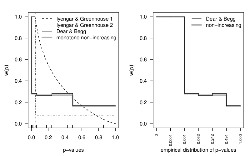
Figure 1: Estimated weight functions for the open classroom education dataset.

Since the nonparametric estimate of Dear and Begg (1992) is already “almost” non-increasing it comes without surprise that the monotone estimate of $w$ is very similar to its unconstrained counterpart. The estimated weight functions clearly indicate publication bias, an observation already made in Dear and Begg (1992, p. 243). This is further supported by the $p$-value computed according to the procedure outlined in Section 6 that amounts to $p_{\text{education}}=0.096$ (for $M=1000$ runs). Now, having an estimate of $w$ at hand yields some more insight in the selection process: According to the monotone estimate, the probability of a $p$-value that is larger than 0.001 to be published is only 28.0% compared to a $p$-value $\leq 0.001$.

Finally, estimates for this dataset from our monotone selection model are $\hat{\theta}=0.14$ and $\hat{\sigma}^{2}=0.11$ with 95% approximate profile likelihood confidence interval for $\theta$ of $[-0.08,0.57]$. Compare these to estimates received from a standard random effects model that amount to $\hat{\theta}=0.26$ and $\hat{\sigma}^{2}=0.30$ with estimated confidence interval for $\theta$ of $[-0.12,0.65]$. The adjustment for selection thus attenuates the effect estimate and narrows the confidence interval but does not change the conclusion about significance of $\theta$ at a significance level of $\alpha=0.05$.

Environmental tobacco smoke data

In our second example we discuss a meta analysis (Hackshaw et al., 1997) of 37 studies concerned with the effect of environmental tobacco smoke on lung-cancer in lifetime non-smokers. The effect in these studies is quantified via the log relative risk. Whether this meta analysis suffers from publication bias has been a matter of ongoing controversy, see Rothstein et al. (2005, p. 91). In the original publication a peculiar form of “failsafe $N$” analysis was conducted and the authors concluded that there is no reason to suspect publication bias. In a re-analysis however, Copas and Shi (2000) (see also the correspondence following that paper on www.bmj.com), applying the method introduced in Copas (1999), came to the conclusion that “the possibility of publication bias cannot be ruled out altogether, and at least some publication bias is needed to explain the trend we found.” However, neither the funnel plot, nor the method by Copas (1999), or Copas and Malley (2008) yields real insight in the nature of the selection process that may be at work. On the other hand, we can estimate the weight function via the unconstrained and the monotone approach, see Figure 2.

First, unlike claimed in Dear and Begg (1992, comment to Figure 2), note that from the unconstrained estimate it is not evident whether publication bias is operating on this dataset.

Again, we can gain some insight in the possible selection mechanism by looking at the estimated weight function which reveals an interesting pattern: One observes four distinct regions which are given by the intervals $[0,0.03]$, $(0.03,0.17]$, $(0.17,0.77]$, $(0.77,1.00]$ where $w$ is constant. These regions are indicated with vertical dashed lines in the left plot of Figure 2. Not surprisingly, sharp drops in the weight function appear around “psychological barriers” for $p$-values, namely 0.05 and maybe 0.15. In passing we remark that discontinuities of the estimated weight function can only happen at actually observed $p$-values.

The probability of selecting a study with $p$-value larger than 0.17 is only 64.8% of that of one with a $p$-value at most 0.17. In addition, the relatively small $p$-value of $p_{\text{tobacco}}=0.13$ computed according the method described in Section 6 reveals some evidence against a constant weight function in Figure 2. For these reasons it seems therefore plausible that publication bias is at work here and we thus agree with the conclusion of Copas and Shi (2000) and Hedges and Vevea (2005, p. 164).

Furthermore, in a standard random effects meta analysis model, we get estimates $\hat{\theta}=0.21$ and $\hat{\sigma}^{2}=0.02$ with estimated confidence interval for $\theta$ of $[0.12,0.31]$. These estimates are attenuated to $\hat{\theta}=0.17$ and $\hat{\sigma}^{2}=0.01$ in the monotone selection model, with 95% approximate profile likelihood confidence interval for $\theta$ of $[0.08,0.26]$. These changes are very similar to those observed by Hedges and Vevea (2005) when choosing their somewhat related weight function. And the significant effect of environmental tobacco smoke on lung cancer persists after adjusting for selection bias.

Finally, to illustrate the computation of the suggested $p$-value, in the lower plot in Figure 2, we have plotted in grey the estimated weight functions for the $M=1000$ samples generated under the assumption of no selection. This gives an impression what selection function can be expected under no selection.

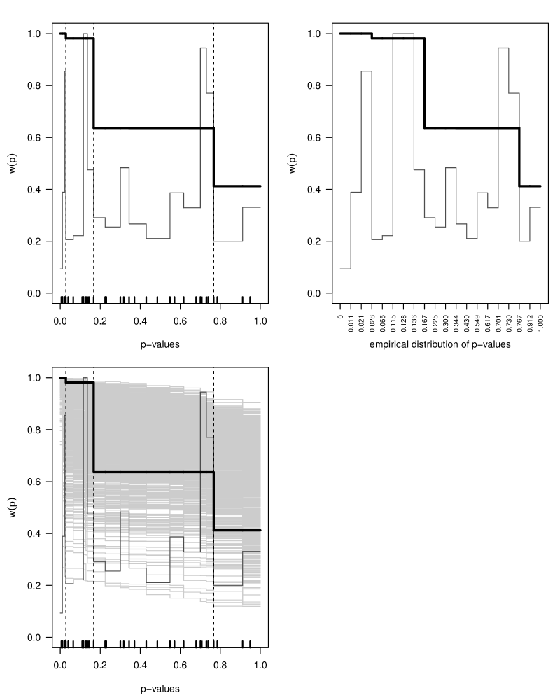
Figure 2: Estimated weight functions for the environmental tobacco smoke dataset ($n=37,k=19$). Thick lines: monotone non-increasing weight functions. Thin lines: Unrestricted weight functions. Dashed vertical lines at 0.03, 0.17, 0.77.

8 Software and reproducibility

Although some of the methods discussed here have been around for some time, it seems as if none of them has found its way in the daily routine of meta analysts. Sutton et al. (2000, p. 439) explain this lack of use by “One of the explanations for this is almost certainly the complexity of many of the approaches (particularly the selection models, and Copas’ approach), and the lack of user-friendly software available to implement them.” In addition, “A further reason for low penetration is possibly lack of acceptance of such methods. and “Selection models are quite sophisticated and there is currently a lack of software to implement them”. To foster the use of selection models by meta analysts we have therefore implemented

• the parametric weight functions $w_{1}$ and $w_{2}$ from Iyengar and Greenhouse (1988) as well as maximum likelihood estimation of their corresponding parameters,

• the nonparametric method of Dear and Begg (1992),

• our new variant that provides a monotone version of the latter estimate, including estimation of the selection bias adjusted estimates of $\theta$ and $\sigma$ as well as the approximate profile likelihood confidence interval for $\theta$,

• the density, distribution, and quantile function as well as random number generation from the $p$-value density (8),

• and the procedure to compute a $p$-value to assess the null hypothesis of no selection introduced in Section 6,

in a new R package selectMeta (Rufibach, 2011) which is available from CRAN. In addition, we provide in selectMeta the two datasets analyzed in Section 7.

Making the software and datasets discussed in this paper accessible enables reproducibility of the results and plots. The code that generates Figures 1 and 2 as well as the computation of the $p$-value introduced in Section 6 for these two examples can be found in the help file for the function DearBegg in selectMeta.

This document was created using Sweave (Leisch, 2002), LaTeX (Knuth, 1984; Lamport, 1994), R 2.12.2 (R Development Core Team, 2010) with the R packages selectMeta (Rufibach, 2011, Version 1.0.3), DEoptim (Ardia and Mullen, 2010, Version 2.0-9), meta (Schwarzer, 2010, Version 1.6-1), reporttools (Rufibach, 2009, Version 1.0.5), and cacheSweave (Peng, 2008, Version 0.4-5).

9 Final remarks

We propose and analyze a new type of monotone frequentist nonparametric weight functions as a visual tool to gain insight in the study selection process when publication bias in meta analysis must be suspected. Selection models have not yet entered the standard toolbox of meta analysts, presumably due to lack of easy accessible software. Our goal was to reduce this gap by collecting many existing and our new approach as functions in a new R package selectMeta (Rufibach, 2011).

More research is necessary to popularize selection models. We intend to develop a smooth version of our new estimator by imposing not only a monotonicity but also a smoothness constraint on the log-likelihood. However, already difficult algorithmic aspects are not facilitated by such additional regularization structure. We further plan to apply and adapt the method of Sun and Woodroofe (1997) to meta analysis. Finally, Hedges and Vevea (2005, Eq. 9.6) describe how to incorporate $\theta$ not only as a simple number, but rather depending on covariates in a regression model. This approach should also allow for a generalization to other than the specific selection model they look at.

Acknowledgments

I thank an external reviewer and the associated editor for valuable comments.

Conflict of Interest

The author has declared no conflict of interest.

Appendix A Derivation of relevant quantities

In this brief appendix, we provide some additional computations that lead to the log-likelihood function, merely for the reader’s convenience. As a matter of fact and since the log-likelihood used in this paper is the one of Dear and Begg (1992), a derivation of $l$ can also be found there. However, here we try to be a bit more explicit.

Since the weight function $w$ is defined to be piecewise constant with values $w_{j}$, the normalizing constants $A_{i}$ simplify to

$$A_{i} = \sum_{j=1}^{k}w_{j}\int_{y:w_{i}(y)=w_{j}}\phi\Bigl{(}\frac{y-\theta}{\eta_{i}}\Bigr{)}\,\mathrm{d}y$$

$$=: \sum_{j=1}^{k}w_{j}H_{ij}.$$

The quantities $H_{ij}$ can be computed as follows:

$$H_{ij} = \int_{y:w_{i}(y)=w_{j}}\phi\Bigl{(}\frac{y-\theta}{\eta_{i}}\Bigr{)}\,\mathrm{d}y$$

$$= \int_{b_{i,2j-2}\leq|y|<b_{i,2j}}\phi\Bigl{(}\frac{y-\theta}{\eta_{i}}\Bigr{)}\,\mathrm{d}y$$

$$= \int_{b_{i,2j-2}}^{b_{i,2j}}\phi\Bigl{(}\frac{y-\theta}{\eta_{i}}\Bigr{)}\,\mathrm{d}y+\int_{-b_{i,2j}}^{-b_{i,2j-2}}\phi\Bigl{(}\frac{y-\theta}{\eta_{i}}\Bigr{)}\,\mathrm{d}y$$

$$= \Phi\Bigl{(}\frac{b_{i,2j}-\theta}{\eta_{i}}\Bigr{)}-\Phi\Bigl{(}\frac{b_{i,2j-2}-\theta}{\eta_{i}}\Bigr{)}+\Phi\Bigl{(}\frac{-b_{i,2j-2}-\theta}{\eta_{i}}\Bigr{)}-\Phi\Bigl{(}\frac{-b_{i,2j}-\theta}{\eta_{i}}\Bigr{)}$$

$$= \Phi(a_{ij})-\Phi(b_{ij})+\Phi(c_{ij})-\Phi(d_{ij})$$

where we defined

$$a_{ij}\ =\ \frac{u_{i}|y_{2j}|/u_{2j}-\theta}{\eta_{i}} b_{ij}\ =\ \frac{u_{i}|y_{2j-2}|/u_{2j-2}-\theta}{\eta_{i}}$$

$$c_{ij}\ =\ \frac{-u_{i}|y_{2j-2}|/u_{2j-2}-\theta}{\eta_{i}} d_{ij}\ =\ \frac{-u_{i}|y_{2j}|/u_{2j}-\theta}{\eta_{i}},$$

see Dear and Begg (1992, Appendix). Consider the following “boundary cases”: Defining $p_{0}=1$ and $p_{2k}=0$, we get $b_{i,0}=0$ and $b_{i,2k}=\infty$, what immediately entails

$$H_{i1} = \Phi\Bigl{(}\frac{b_{i,2j}-\theta}{\eta_{i}}\Bigr{)}-\Phi\Bigl{(}\frac{-\theta}{\eta_{i}}\Bigr{)}+\Phi\Bigl{(}\frac{-\theta}{\eta_{i}}\Bigr{)}-\Phi\Bigl{(}\frac{-b_{i,2j}-\theta}{\eta_{i}}\Bigr{)}$$

$$= \Phi\Bigl{(}\frac{u_{i}|y_{2}|/u_{2}-\theta}{\eta_{i}}\Bigr{)}-\Phi\Bigl{(}\frac{-u_{i}|y_{2}|/u_{2}-\theta}{\eta_{i}}\Bigr{)}\ =\ \Phi(a_{i1})-\Phi(d_{i1}).$$

On the other hand,

$$H_{ik} = \Phi\Bigl{(}\frac{b_{i,2k}-\theta}{\eta_{i}}\Bigr{)}-\Phi\Bigl{(}\frac{b_{i,2k-2}-\theta}{\eta_{i}}\Bigr{)}+\Phi\Bigl{(}\frac{-b_{i,2k-2}-\theta}{\eta_{i}}\Bigr{)}-\Phi\Bigl{(}\frac{-b_{i,2k}-\theta}{\eta_{i}}\Bigr{)}$$

$$= 1-\Phi\Bigl{(}\frac{u_{i}|y_{2k-2}|/u_{2k-2}-\theta}{\eta_{i}}\Bigr{)}+\Phi\Bigl{(}\frac{-u_{i}|y_{2k-2}|/u_{2k-2}-\theta}{\eta_{i}}\Bigr{)}\ =\ 1-\Phi(b_{ik})+\Phi(c_{ik}).$$

Plugging all the above quantities into (1), the log-likelihood function amounts to

$$l(\boldsymbol{w},\theta,\sigma^{2}) = \log L(\boldsymbol{w},\theta,\sigma^{2})$$

$$= \sum_{i=1}^{n}\log w_{i}(y_{i})+\sum_{i=1}^{n}\log\Bigl{\{}\eta_{i}^{-1}\phi\Bigl{(}\frac{y_{i}-\theta}{\eta_{i}}\Bigr{)}\Bigr{\}}-\sum_{i=1}^{n}\log\Bigl{(}\sum_{j=1}^{k}w_{j}H_{ij}\Bigr{)}$$

$$= -\frac{n}{2}\log(2\pi)+\sum_{j=1}^{k}\lambda_{j}\log w_{j}-\sum_{i=1}^{n}\log\eta_{i}-\frac{1}{2}\sum_{i=1}^{n}\Bigl{(}\frac{y_{i}-\theta}{\eta_{i}}\Bigr{)}^{2}-\sum_{i=1}^{n}\log A_{i}.$$

References

- Ardia and Mullen (2010) Ardia, D. and Mullen, K. (2010). DEoptim: Differential Evolution Optimization in R. R package version 2.0-7.
- Carpenter et al. (2009) Carpenter, J., Rücker, G. and Schwarzer, G. (2009). copas: An R package for Fitting the Copas Selection Model. The R Journal 1 31–36.
- Copas (1999) Copas, J. (1999). What works?: selectivity models and meta-analysis. Journal of the Royal Statistical Society, Series C (Applied Statistics) 162 95–109.
- Copas and Malley (2008) Copas, J. B. and Malley, P. F. (2008). A robust p-value for treatment effect in meta-analysis with publication bias. Statistics in Medicine 27 4267–4278.
- Copas and Shi (2000) Copas, J. B. and Shi, J. Q. (2000). Reanalysis of epidemiological evidence on lung cancer and passive smoking. British Medical Journal 320 417–418.
- Copas and Shi (2001) Copas, J. B. and Shi, J. Q. (2001). A sensitivity analysis for publication bias in systematic reviews. Statistical Methods in Medical Research 10 251–265.
- Dear and Begg (1992) Dear, K. B. and Begg, C. B. (1992). An Approach for Assessing Publication Bias Prior to Performing a Meta-Analysis. Statistical Science 7 237–245.
- Fan and Wong (2000) Fan, J. and Wong, W. (2000). Discussion of “on profile likelihood” by murphy and van der vaart. Journal of the American Statistical Association 95 468–471.
- Ghosh (2007) Ghosh, D. (2007). Incorporating monotonicity into the evaluation of a biomarker. Biostatistics 8 402–413.
- Givens et al. (1997) Givens, G., Smith, D. and Tweedie, R. (1997). Publication bias in meta-analysis: A Bayesian data-augmentation approach to account for issues exemplified in the passive smoking debate. Statistical Science 12 221–240.
- Hackshaw et al. (1997) Hackshaw, A. K., Law, M. R. and Wald, N. J. (1997). The accumulated evidence on lung cancer and environmental tobacco smoke. British Medical Journal 315 980–988.
- Hedges (1984) Hedges, L. (1984). Estimation of effect size under nonrandom sampling: the effects of censoring studies yielding statistically significant mean differences. Journal of Educational Statistics 3 109–135.
- Hedges (1988) Hedges, L. (1988). Comment to the article “selection models and the file drawer problem”. Statistical Science 3 118–120.
- Hedges (1992) Hedges, L. V. (1992). Modeling Publication Selection Effects in Meta-Analysis. Statistical Science 7 246–255.
- Hedges and Olkin (1985) Hedges, L. V. and Olkin, I. (1985). Statistical methods for meta-analysis. Academic Press Inc., Orlando, FL.
- Hedges and Vevea (2005) Hedges, L. V. and Vevea, J. (2005). Selection method approaches. In Publication bias in meta-analysis (H. Rothstein, A. J. Sutton and M. Borenstein, eds.). John Wiley & Sons Ltd., Chichester, Chapter 9, p. 145–174.
- Hedges and Vevea (1996) Hedges, L. V. and Vevea, J. L. (1996). Estimating effect size under publication bias: Small sample properties and robustness of a random effects selection model. Journal of Educational and Behavioral Statistics 21 pp. 299–332.
- Iyengar and Greenhouse (1988) Iyengar, S. and Greenhouse, J. B. (1988). Selection models and the file drawer problem. Statistical Science 3 109–135.
- Iyengar and Zhao (1994) Iyengar, S. and Zhao, P. L. (1994). Maximum likelihood estimation for weighted distributions. Statistics & Probability Letters 21 37–47.
- Kelly (1989) Kelly, R. E. (1989). Stochastic reduction of loss in estimating normal means by isotonic regression. Annals of Statistics 17 937–940.
- Knuth (1984) Knuth, D. (1984). Literate programming. Computer Journal 27 97–111.
- Lamport (1994) Lamport, L. (1994). LaTeX: A Document Preparation System. 2nd ed. Addison-Wesley, Reading, Massachusetts.
- Lee (2001) Lee, J. (2001). On posterior consistency in selection models. Statistica Sinica 11 827–842.
- Leisch (2002) Leisch, F. (2002). Dynamic generation of statistical reports using literate data analysis. In COMPSTAT 2002 – Proceedings in Computational Statistics (W. Härdle and B. Rönz, eds.). Physica Verlag, Heidelberg.
- Macaskill et al. (2001) Macaskill, P., Walter, S. D. and Irwig, L. (2001). A comparison of methods to detect publication bias in meta-analysis. Statistics in Medicine 20 641–654.
- Murphy and van der Vaart (2000) Murphy, S. A. and van der Vaart, A. W. (2000). On profile likelihood. Journal of the American Statistical Association 95 449–485. With comments and a rejoinder by the authors.
- Peng (2008) Peng, R. D. (2008). Caching and distributing statistical analyses in R. Journal of Statistical Software 26 1–24.
- Preston et al. (2004) Preston, C., Ashby, D. and Smyth, R. (2004). Adjusting for publication bias: modelling the selection process. Journal of Evaluation in Clinical Practice 10 313–322.
- R Development Core Team (2010) R Development Core Team (2010). R: A Language and Environment for Statistical Computing. R Foundation for Statistical Computing, Vienna, Austria. ISBN 3-900051-07-0.
- Rothstein et al. (2005) Rothstein, H. R., Sutton, A. J. and Borenstein, M. (eds.) (2005). Publication bias in meta-analysis. John Wiley & Sons Ltd., Chichester. Prevention, assessment and adjustments.
- Rufibach (2009) Rufibach, K. (2009). reporttools: R functions to generate LaTeX tables of descriptive statistics. Journal of Statistical Software, Code Snippets 31.
- Rufibach (2011) Rufibach, K. (2011). selectMeta: Estimation of weight functions in meta analysis. R package version 1.0-2.
-
Schwarzer (2010)
Schwarzer, G. (2010).
meta: Meta-Analysis with R.
R package version 1.6-1.
URL http://CRAN.R-project.org/package=meta - Silliman (1997a) Silliman, N. P. (1997a). Hierarchical selection models with applications in meta-analysis. Journal of the American Statistical Association 92 926–936.
- Silliman (1997b) Silliman, N. P. (1997b). Nonparametric classes of weight functions to model publication bias. Biometrika 84 909–918.
- Storn and Price (1997) Storn, R. and Price, K. (1997). Differential evolution—a simple and efficient heuristic for global optimization over continuous spaces. Journal of Global Optimization 11 341–359.
- Sun and Woodroofe (1997) Sun, J. and Woodroofe, M. (1997). Semi-parametric estimates under biased sampling. Statistica Sinica 7 545–575.
- Sutton and Higgins (2008) Sutton, A. J. and Higgins, J. P. I. (2008). Recent developments in meta-analysis. Statistics in Medicine 27 625–650.
- Sutton et al. (2000) Sutton, A. J., Song, F., Gilbody, S. M. and Abrams, K. R. (2000). Modelling publication bias in meta-analysis: a review. Statistical Methods in Medical Research 9 421–445.
- Woodroofe and Sun (1999) Woodroofe, M. and Sun, J. (1999). Testing uniformity versus a monotone density. Annals of Statistics 27 338–360.