Nodeless energy gaps of single-crystalline Ba_0.68K_0.32Fe₂As₂ as seen via ⁷⁵As NMR

Abstract

We report ⁷⁵As nuclear magnetic resonance studies on a very clean hole-doped single-crystal Ba_0.68K_0.32Fe₂As₂ ($T_{\rm{c}}=38.5$ K). The spin-lattice relaxation rate $1/T_{1}$ shows an exponential decrease below $T\simeq 0.45T_{\rm c}$ down to $T\simeq 0.11T_{\rm c}$, which indicates a fully-opened energy gap. From the ratio $(T_{1})_{c}/(T_{1})_{a}$, where $a$ and $c$ denote the crystal directions, we find that the antiferromagnetic spin fluctuation is anisotropic in the spin space above $T_{\rm c}$. The anisotropy decreases below $T_{\rm c}$ and disappears at $T\rightarrow 0$. We argue that the anisotropy stems from spin-orbit coupling whose effect vanishes when spin-singlet electron pairs form with a nodeless gap.

The discovery of superconducting transition in electron-doped iron-arsenide LaFeAsO_1-xF_x provides a new route to high temperature superconductivity YKamihara . Remarkably, many other $R$FeAsO_1-xF_x ($R$: rare earth) were synthesized and $T_{\rm{c}}$ was raised to 55 K in SmFeAsO_1-xF_x ZARenSm , which is the highest among materials except cuprates. Soon after these works, the hole-doped BaFe₂As₂ was also found to be superconducting 122 . The large single crystals of Ba_1-xK_xFe₂As₂ are easy to obtain, which makes them a good system for studying many physical quantities.

One of the most outstanding issues for a new superconductor is the symmetry of the electron pairs which is directly related to the paring mechanism. Nuclear magnetic resonance (NMR) experiments found the electron pairs to be in the spin-singlet state KMatanoPr and indicated the existence of multiple energy gaps KMatanoPr ; SKawasaki . The multiple-gap property is likely associated with the multiple electronic bands. The Fermi surfaces consist of two hole-pockets centered at the $\Gamma$ point and two electron pockets around the $M$ point DJSingh . However, whether there are nodes in the gap function or not is still under hot debate. Angle-resolved photoemission spectroscopy (ARPES) HDing suggested fully opened gaps, but thermal conductivity LiSL ; Taillefer measurements suggested nodal gaps. The penetration depth measurements by different groups have led to opposite conclusions KHashimoto ; CMartin .

Theoretically, the sign-reversing $s^{\pm}$-wave model has been considered as the most promising candidate IIMazin ; kuroki ; fwang , but $d$ wave or $s$ wave with zero gap, and even a conventional $s^{++}$ wave was also proposed SGraser ; Thomale ; Kontani . It has been shown that the $s^{\pm}$-wave or a multiple-gap $d$-wave model can fit quite well the spin-lattice relaxation rate, $1/T_{1}$, which shows a rapid decrease below $T_{\rm c}$ with a hump structure at $T\sim T_{\rm c}/2$ KMatanoPr ; SKawasaki ; YBang ; parish ; KMatanoBa . However, an important feature that $1/T_{1}$ should decrease as an exponential function of $T$ expected for the $s$-wave gaps has not been observed so far, because of impurity scattering in the samples. The impurity scattering can also alter other physical properties Johnston . Thus, the conclusions on the gap symmetry drawn so far are still controversial. Measurements in sufficiently clean samples are highly needed to resolve the issue.

Here we report ⁷⁵As NMR study on a very clean single crystal Ba_0.68K_0.32Fe₂As₂ with $T_{c}=38.5$ K that is the highest among reports for this family. We obtained two pieces of evidence for fully-opened gaps. First, we observe an exponential decay of $1/T_{1}$ below $T\simeq 0.45T_{\rm c}$ down to $T\simeq 0.11T_{\rm c}$. For the second piece of evidence, we find that the antiferromagnetic (AF) spin fluctuation (SF) is anisotropic in the spin space above $T_{\rm c}$, but the anisotropy decreases below $T_{\rm c}$ and disappears at $T\rightarrow 0$. We argue that the anisotropy is due to spin-orbit coupling, whose effect vanishes at $T\rightarrow 0$ because the electron pairs are in the spin-singlet state with nodeless gap.

The single crystal of Ba_0.68K_0.32Fe₂As₂ was grown by using the self-flux method and characterized as discussed elsewhere GLSun . Both dc susceptibility measured by a superconducting quantum interference device and ac susceptibility measured by the NMR coil indicates $T_{\rm{c}}=38.5$ K at zero magnetic field. The $T_{\rm{c}}$ is 37.6 K for $\mu_{0}H$ (=7.5T) $\parallel a$ axis and 36.4 K for $\mu_{0}H$ (=7.5T) $\parallel c$ axis. The $1/T_{1}$ was determined from an excellent fitting to $1-M(t)/M(\infty)=0.1$exp$(-t/T_{1})+0.9$ exp$(-6t/T_{1})$, where $M(t)$ is the nuclear magnetization at time $t$ after the saturation pulse ANarath .

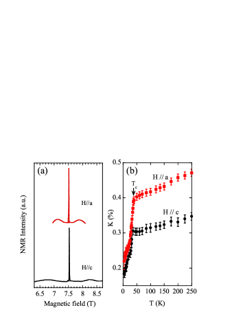
Figure 1: (Color online) (a) ⁷⁵As-NMR spectra at a frequency of $\omega_{0}/2\pi=55.1$ MHz and $T$=100 K. The vertical axis for $H\parallel a$ is offset for clarity. (b) The $T$ dependence of the Knight shift with $H\parallel a$ axis and $H\parallel c$ axis, respectively. The arrow indicates $T_{\rm c}$ for $H\parallel a$.

Figure 1 (a) shows the ⁷⁵As-NMR spectra by scanning the magnetic field at a fixed frequency, $\omega_{0}/2\pi=55.1$ MHz. The nuclear quadrupole frequency $\nu_{Q}$ is found to be 5.1 MHz at 100 K which is smaller than that in the Sn-flux-grown sample (5.9 MHz) KMatanoBa . Since doping of K increases $\nu_{Q}$ KMatanoBa , this suggests that the Sn-flux-grown crystal had a higher doping rate. The Knight shift $K$ was obtained from the central transition peak and determined with respect to $\omega_{0}/\gamma$ with the nuclear gyromagnetic ratio $\gamma=7.2919$ MHz/T. Below $T_{\rm c}$, $K$ is obtained by scanning $\omega_{0}$ at a fixed field to avoid the vortex pinning effect. Above $T_{\rm c}$, we confirmed that the results obtained by scanning field and scanning frequency agree well. The effect of the nuclear quadrupole interaction was taken into account in extracting $K_{a}$. As shown in Fig. 1 (b), both $K_{a}$ and $K_{c}$ show a sharp decrease below $T_{\rm c}$, which indicates spin-singlet pairing KMatanoPr .

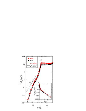
Figure 2: (Color online) The $T$ dependence of $1/T_{1}$. The error is within the size of the symbols. The dashed line shows the $T^{3}$ variation. The curves below $T_{\rm{c}}$ are fits to a two-gap $s^{\pm}$ model using the same parameters for both directions. The inset shows the semilog plot of $1/T_{1}T$ vs $T_{\rm c}/T$, which evidences an activation type $T$ dependence of the relaxation..

The main panel of Fig. 2 shows the $T$ dependence of $1/T_{1}$ that decreases rapidly below $T_{\rm c}$, with the reduction over about five decades. The decrease at low $T$ is much faster than $T^{3}$ that is expected for a $d$-wave gap. As in other materials, $1/T_{1}$ shows a “knee” shape around half $T_{\rm{c}}$, which indicates multiple gaps KMatanoPr ; SKawasaki . To see the low-$T$ behavior more clearly, we plot $1/T_{1}T$ as a function of inverse reduced-temperature $T_{\rm{c}}/T$ in the inset. As can be seen there, $1/T_{1}T$ shows a very good exponential behavior below 17 K. This is strong evidence for a fully opened gap.

Using the $s^{\pm}$-wave model and introducing the impurity scattering rate $\eta$ in the energy spectrum, $E=\omega+i\eta$ ZLi , but neglecting the quasiparticle damping effect for simplicity, we can fit the data quite well. For a sign-reversing two-gap model, as seen in Fig. 2, we obtain $\Delta_{1}^{+}=5.63$ $k_{\rm{B}}T_{\rm{c}}$, $\Delta_{2}^{-}=1.11$ $k_{\rm{B}}T_{\rm{c}}$, $N_{1}:N_{2}=0.85:0.15$, where $N_{i}$ is the density of state (DOS) on band $i$, and $\eta=0.044$ $k_{\rm B}T_{\rm c}$. For a model of three bands corresponding to ARPES HDing , we obtain $\Delta_{1}^{+}=4.7$ $k_{\rm{B}}T_{\rm{c}}$, $\Delta_{2}^{+}=0.96$ $k_{\rm{B}}T_{\rm{c}}$, $\Delta_{3}^{-}=4.7$ $k_{\rm{B}}T_{\rm{c}}$, $N_{1}:N_{2}:N_{3}=0.44:0.12:0.44$, and $\eta=0.022$ $k_{\rm B}T_{\rm c}$. The $\eta$ is much smaller than $\eta=0.15$ $k_{\rm B}T_{\rm c}$ in LaFeAsO_0.92F_0.08 SKawasaki and $\eta=0.22$ $k_{\rm B}T_{\rm c}$ in the Sn-flux grown Ba_0.72K_0.28Fe₂As₂ KMatanoBa , meaning that the present sample is much cleaner, as supported by a small resistivity of 26$\mu$$\Omega$ at $T_{c}$ GLSun and the much sharper spectrum-width that is only half the value for the Sn-flux grown crystal. The cleanness of the present crystal is the reason for the exponential behavior of $1/T_{1}$ at low $T$; impurity scattering brings about finite DOS that results in seemingly power-law $T$-dependence of $1/T_{1}$ KMatanoPr ; ZLi ; Grafe ; Fukazawa ; Yashima . It should be emphasized that the coherence peak is not seen even in such clean sample, which seems hard to be explained by a $s^{++}$-wave gap.

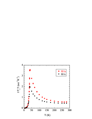
Figure 3: (Color online) $T$-dependence of the ${}^{75}(1/T_{1}T)$. The arrow indicates $T_{c}$.

Next we move to the normal state. Figure 3 shows the $T$ dependence of $1/T_{1}T$ which increases with decreasing $T$ down to $T_{\rm c}$, indicating strong AF SF. The $1/T_{1}T$ stems from the magnetic susceptibility at all wave vectors. When there exists strong AF SF, one may assume $1/T_{1}T=(1/T_{1}T)^{\rm AF}+(1/T_{1}T)^{0}$, where $(1/T_{1}T)^{\rm AF}$ is due to the susceptibility at the AF wave vector $Q$, and $(1/T_{1}T)^{0}$ is due to $s$-band electrons and the orbital hyperfine interaction. Note that above $T=250$K, $1/T_{1}T$ becomes a constant. By taking the averaged value of $1/T_{1}T$ at $T\geq 250$K as $(1/T_{1}T)^{0}$, $(1/T_{1}T)^{\rm AF}$ is then obtained. Figure 4 shows the ratio of the relaxation due to AF SF, $(T_{1})_{c}^{\rm AF}/(T_{1})_{a}^{\rm AF}$, which is about $2$. This result indicates that the SF is anisotropic in the spin space, as elaborated below.

Generally, $1/T_{1}$ is related to the transverse fluctuating internal magnetic field, $\delta H$, as follows TMoriya :

$$\left(\frac{1}{T_{1}}\right)_{z}= \frac{\gamma^{2}}{2}\int_{-\infty}^{\infty}{\rm d}t{\rm cos}(\omega_{0}t) \left<\delta H_{x}(t)\delta H_{x}(0)+\delta H_{y}(t)\delta H_{y}(0)\right>,$$ (1)

where $\left<\cdots\right>$ denotes the statistical average. $\delta{\bf H}$ is related to the fluctuating moment ${\bf S}$ of Fe as $\delta{\bf H}={\bf A}\cdot{\bf S}$, where ${\bf A}$ is the hyperfine coupling tensor between the As nucleus and Fe spins.

For $Q=(\pi,0)$ and $Q=(0,\pi)$ AF SF, one has KKitagawa

$${\bf A}(\pi,0)=\left(\begin{array}[]{ccc}0&0&A\\ 0&0&0\\ A&0&0\\ \end{array}\right),\ \ {\rm and}\ \ {\bf A}(0,\pi)=\left(\begin{array}[]{ccc}0&0&0\\ 0&0&A\\ 0&A&0\\ \end{array}\right),$$ (8)

respectively. One therefore obtains

$$(1/T_{1})_{a,b}^{\rm AF} = \frac{\gamma^{2}}{4}A^{2}\int_{-\infty}^{\infty}{\rm d}t{\rm cos}(\omega_{0}t)\left<S_{a}(t)S_{a}(0)+S_{b}(t)S_{b}(0)+S_{c}(t)S_{c}(0)\right>,$$ (9)

$$(1/T_{1})_{c}^{\rm AF} = \frac{\gamma^{2}}{2}A^{2}\int_{-\infty}^{\infty}{\rm d}t{\rm cos}(\omega_{0}t)\left<S_{c}(t)S_{c}(0)\right>.$$ (10)

Since $\left<S_{j}(t)S_{j}(0)\right>$ $(j=a,b,c)$ can be expressed in terms of the imaginary part of the susceptibility $\chi^{\prime\prime}_{j}$ through the fluctuation-dissipation theorem, $\int_{-\infty}^{\infty}{\rm d}t{\rm cos}(\omega_{0}t)\left<S_{j}(t)S_{j}(0)\right>=\frac{2k_{\rm B}T\chi^{\prime\prime}_{j}(\omega_{0})}{(\gamma_{e}\hbar)^{2}\omega_{0}}$ , the anisotropy of the relaxation can be expressed as

$$R_{\rm AF}=\frac{(1/T_{1})_{a}^{\rm AF}}{(1/T_{1})_{c}^{\rm AF}}=\frac{\chi^{\prime\prime}_{a}(\omega_{0},Q)+\chi^{\prime\prime}_{b}(\omega_{0},Q)}{2\chi^{\prime\prime}_{c}(\omega_{0},Q)}+\frac{1}{2}.$$ (11)

If $\chi^{\prime\prime}_{a}(\omega_{0},Q)=\chi^{\prime\prime}_{b}(\omega_{0},Q)=\chi^{\prime\prime}_{c}(\omega_{0},Q)$, namely, if the SF is isotropic in the spin space, then

$$R_{\rm AF}^{\rm iso}=1.5.$$ (12)

The observed $R_{\rm AF}$ shown in Fig. 4 is much larger than 1.5, which follows from Eq. (5) that $\chi^{\prime\prime}_{a,b}(\omega_{0},Q)$ is larger than $\chi^{\prime\prime}_{c}(\omega_{0},Q)$ by about 50%.

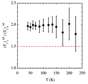
Figure 4: (Color online) $T$-dependence of the anisotropy of $T_{1}$ due to AF spin fluctuation. The dashed line marks the value for isotropic AF spin fluctuation.

We propose that the anisotropy in the SF stems from spin-orbit coupling (SOC) that mixes spin and orbital freedoms so that the magnetic susceptibility bears some orbital character, which is anisotropic. We use a two-band model SRaghu involving spin-orbit coupled $d_{xz}$ and $d_{yz}$ and calculate the anisotropy. Our theoretical study starts from a two-dimensional Hamiltonian:

$$H=H_{TB}+H_{LS}.$$ (13)

Here $H_{TB}=\sum_{\mathbf{k}\mu\nu\sigma}\varepsilon_{\mu\nu}d^{{\dagger}}_{\mathbf{k}\mu\sigma}d_{\mathbf{k}\nu\sigma}$ is the tight-binding Hamiltonian with orbit index $\mu,\nu=1(xz),2(yz)$ and spin index $\sigma=+1(\uparrow),-1(\downarrow)$. The SOC is described by $H_{LS}=2\lambda_{LS}\sum_{l}\mathbf{L}_{l}\cdot\mathbf{S}_{l}=-i\lambda_{LS}\sum_{\mathbf{k}\sigma}\sigma d^{{\dagger}}_{\mathbf{k},1\sigma}d_{\mathbf{k},2\sigma}+h.c.$ .

The dynamical magnetic response is calculated at the random-phase-approximation level, with the on-site intra-orbit Hubbard interaction $H_{U}=\sum_{l\in Lattice,\mu}Un_{l\mu\uparrow}n_{l\mu\downarrow}$. The longitudinal (transverse) susceptibility $\bar{\chi}_{c}$ ($\bar{\chi}_{+-}$) at $\mathbf{q}$=$\mathbf{Q}=(\pi,0)$ or $(0,\pi)$ is

$$\bar{\chi}_{c(+-)}(\mathbf{q},i\nu_{n})=\frac{1}{1-\bar{\chi}_{0,c(+-)}(\mathbf{q},i\nu_{n})\Gamma(\mathbf{q})}\bar{\chi}_{0,c(+-)}(\mathbf{q},i\nu_{n}),$$ (14)

where $\bar{\chi}$ is a $2\times 2$ matrix in the orbital space with the matrix elements defined by $\bar{\chi}_{c}^{\mu\nu}(\mathbf{q},\tau)=\langle T_{\tau}S^{z}_{\mu}(-\mathbf{q},\tau)S^{z}_{\nu}(\mathbf{q},0)\rangle$ and $\bar{\chi}_{+-}^{\mu\nu}(\mathbf{q},\tau)=\frac{1}{2}\langle T_{\tau}S^{+}_{\mu}(-\mathbf{q},\tau)S^{-}_{\nu}(\mathbf{q},0)\rangle$. $\Gamma(\mathbf{q})=\text{diag}(U,U)$ is the Hubbard interaction vertex in the spin-spin channel. The bare susceptibility $\bar{\chi}_{0}(\mathbf{q},i\nu_{n})$ can be easily obtained by diagonalizing the Hamiltonian shown in Eq. (7). We choose the nearest-neighbor hopping integral $t_{1}=-0.1051$ eV More2009 .

The calculated magnetic anisotropy above $T_{c}$ with $\lambda$=0.2$|t_{1}|$ ($U=9.7|t_{1}|$) and $\lambda$=0.1$|t_{1}|$ ($U=9.87|t_{1}|$), leading to $R_{AF}\sim$2 at $T=T_{c}$, is respectively shown in Fig. 5, which is in qualitative agreement with the experimental finding. Here $T_{c}$=0.065$|t_{1}|$ is obtained by a self-consistent calculation of a mean-field BCS model with a gap $\Delta=0.309|t_{1}|$.

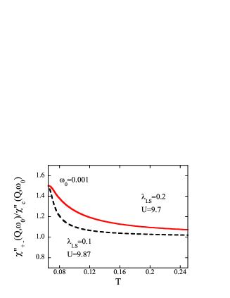
Figure 5: (Color online) Calculated magnetic anisotropy above $T_{c}$ due to SOC. The parameters and $k_{B}T$ are in units of $|t_{1}|$, where $t_{1}$ is the nearest-neighbor hopping integral.

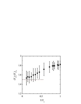
Figure 6: (Color online) $T$-dependence of the $T_{1}$ anisotropy below $T_{c}$. The dashed straight line indicates the value for isotropic AF SF.

A particular feature we find experimentally is that the $T_{1}$ ratio decreases below $T_{\rm c}$ and it approaches the characteristic value $1.5$ for the isotropic SF. Below $T_{\rm c}$, it is less trivial to subtract the contribution of $(1/T_{1}T)^{0}$, so we simply plot the raw data as shown in Fig. 6. We emphasize, however, that this approximation does not affect our conclusion footnote , since the contribution from $(1/T_{1}T)^{0}$ to the observed $1/T_{1}T$ is only $15\%$ for $H\parallel a$ and $20\%$ for $H\parallel c$ at $T=T_{\rm c}$.

The asymptotic value $1.5$ for $(T_{1})_{c}/(T_{1})_{a}$ implies that the SOC effect vanishes at $T\rightarrow 0$. This can happen only when the gaps are fully opened in the case of spin-singlet pairing with $\Delta>\lambda_{\rm LS}$. When there are nodes in the gap function, $1/T_{1}$ at low $T$ is governed by the nodal quasiparticles that are spin-orbit coupled, thereby $(T_{1})_{c}/(T_{1})_{a}$ should resume its value of $2.0$ at $T=T_{\rm c}$. Note also that $(T_{1})_{c}/(T_{1})_{a}$ should become $\sim$0.75 if the AF SF completely vanishes KKitagawa . Thus, our finding of the decrease of $(T_{1})_{c}/(T_{1})_{a}$ to $1.5$ at $T\rightarrow 0$ is another strong evidence for nodeless gap and implies that the AF SF persists in the superconducting state.

In conclusion, from the NMR measurements on a clean single crystal Ba_0.68K_0.32Fe₂As₂, we find the long-sought exponential decrease of $1/T_{1}$ at low $T$, which evidences a fully-opened gap. In the normal state, the AF SF is anisotropic in the spin space. However, the anisotropy diminishes below $T_{\rm c}$ and vanishes at the zero-$T$ limit, which is a feature indicating nodeless gap.

We thank S. Kawasaki, K. Matano and M. Ichioka for help, and I. Eremin, Z. Fang, H. Ikeda and Z.-Y. Lu for useful discussions. This work was supported by CAS, research grants from JSPS and MEXT, and NSFC No. 10974167 (YHS).

References

(1)
Y. Kamihara et al., J. Ame. Chem. Soc. 130, 3296 (2008).
(2)
Z. A. Ren et al., Chin. Phys. Lett. 25, 2215 (2008).
(3)
M. Rotter et al., Phys. Rev. Lett. 101, 107006 (2008).
(4)
K. Matano et al., Europhys. Lett. 83, 57001 (2008).
(5)
S. Kawasaki et al., Phys. Rev. B 78, 220506 (2008).
(6)
D. J. Singh et al.,
Phys. Rev. Lett. 100, 237003 (2008).
(7)
H. Ding et al., Europhys. Lett. 83, 47001 (2008).
(8)
J. K. Dong et al.,
Phys. Rev. Lett. 104, 087005 (2010).
(9)
J.-Ph. Reid et al.,
Phys. Rew. B 82, 064501 (2010).
(10)
K. Hashimoto et al., Phys. Rev. Lett. 102, 017002 (2009).
(11)
C. Martin et al., Phys. Rev. Lett. 102, 247002 (2009).
(12)
I. I. Mazin et al., Phys. Rev. Lett. 101, 057003 (2008).
(13) K. Kuroki et al.
, Phys. Rev. Lett. 101, 087004 (2008).
(14) F. Wang et al., Phys. Rev. Lett. 102, 047005 (2009).
(15)
S. Graser et al., New. J. Phys. 11, 025016 (2009).
(16)
R. Thomale, et al., Phys. Rev. B 80,
180505(R) (2009).
(17)
H. Kontani and S. Onari, Phys. Rev. Lett. 104, 157001 (2010).
(18)
Y. Bang and H. Y. Choi, Phys. Rev. B 78 134523 (2008).
(19) M. M. Parish et al., Phys. Rev. B 78, 144514
(2008).
(20)
K. Matano et al., Europhys. Lett. 87, 27012 (2009).
(21)
D. C. Johnston, Adv. Phys. 59, 803 (2010).
(22)
G. L. Sun et al., arXiv 0901, 2728v3 (2009).
(23)
A. Narath, Phys. Rev., 162 320 (1967).
(24)
Z. Li et al., J. Phys. Soc. Jpn. 79, 083702 (2010).
(25)
H.-J. Grafe et al., Phys. Rev. Lett. 101, 047003 (2008).
(26)
H. Fukazawa et al.,
J. Phys. Soc. Jpn. 78, 033704 (2009).
(27)
M. Yashima et al., J. Phys. Soc. Jpn. 78, 103702 (2009).
(28)
T. Moriya, J. Phys. Soc. Jpn. 18, 516 (1963).
(29)
K. Kitagawa et al., J. Phys. Soc. Jpn. 77, 114709 (2008).
(30)
S. Raghu et al., Phys. Rev. B 77, 220503 (2008).
(31)
A. Moreo et al.,
Phys. Rev. B 79, 134502(2009).
(32)
Below , if we assume that follows a function as shown by the solid curve in Fig. 2 and subtract it from , then decreases from 2 at to at the lowest temperature .