Frustration-Induced Ferrimagnetism in $S=1/2$ Heisenberg Spin Chain

Abstract

The ground-state properties of the $S=1/2$ frustrated Heisenberg spin chain with interactions up to fourth nearest neighbors are investigated by the exact-diagonalization method and density matrix renormalization group method. Our numerical calculations clarify that the ferrimagnetic state is realized in the ground state in spite of the fact that a multi-sublattice structure in the shape of the system is absent. We find that there are two types of ferrimagnetic phases: one is the well-known ferrimagnetic phase of the Lieb-Mattis type and the other is the nontrivial ferrimagnetic phase that is different from that of the Lieb-Mattis type. Our results suggest that a multi-sublattice structure of the shape is not necessarily required for the occurrence of ferrimagnetism.

Ferrimagnetism is one of fundamental phenomena in the field of magnetism. A typical case showing ferrimagnetism is that when a system includes spins of two types that antiferromagnetically interact between two spins of different types in each neighboring pair. The simplest example is an ($S$, $s$)=($1$, $1/2$) antiferromagnetic mixed spin chain, in which two different spins are arranged alternately in a line and coupled by the nearest-neighbor antiferromagnetic interaction[1]. The occurrence of ferrimagnetism in this case is understood within the Marshall-Lieb-Mattis theorem concerning quantum spin systems[2, 3]. Even though a system includes spins of one type, this theorem also derives the presence of ferrimagnetism when the system includes more than one sublattice of spin sites, for example, the spin system in a diamond chain [4, 5, 6, 7, 8]. From these two mechanisms, the existence of a multi-sublattice structure is very important for the occurrence of ferrimagnetism.

At this stage, one asks a fundamental question: Is a multi-sublattice structure in the shape of a Hamiltonian essential and necessary for the occurrence of ferrimagnetism? The purpose of the present study is to answer this question. Our following demonstration will clarify that the answer is no. In this study, we find that ferrimagnetism can appear due to the effect of magnetic frustration even in the absence of a multi-sublattice structure in the shape of a system.

In this study, we examine the model whose Hamiltonian is given by

$$\mathcal{H} = J\sum_{i}[{\bf S}_{i}\cdot{\bf S}_{i+1}+\frac{1}{2}{\bf S}_{i}\cdot{\bf S}_{i+2}]$$

$$- J^{\prime}\sum_{i}[{\bf S}_{i}\cdot{\bf S}_{i+3}+\frac{1}{2}({\bf S}_{i}\cdot{\bf S}_{i+2}+{\bf S}_{i}\cdot{\bf S}_{i+4})],$$

where ${\bf S}_{i}$ is the $S=1/2$ spin operator at the site $i$. The system size is denoted by $N$. We emphasize here that this model has only one spin in a unit cell, namely, it has no sublattice structure. Energies are measured in units of $J$; therefore, we set $J=1$ hereafter. We have a controllable parameter, $J^{\prime}$, in the Hamiltonian (Frustration-Induced Ferrimagnetism in $S=1/2$ Heisenberg Spin Chain ). This model was originally introduced in ref. References detailing the study of constructing a model Hamiltonian as a generalization from the Majumdar-Ghosh model[12]. The Hamiltonian (Frustration-Induced Ferrimagnetism in $S=1/2$ Heisenberg Spin Chain ) includes two cases in which the ground state of the system is exactly obtained. For $J^{\prime}=0$, the system is reduced to the Majumdar-Ghosh model[12], whose ground state is described by direct products of spin-singlet states in nearest-neighbor pairs of $S=1/2$ spins. The ground state is called the dimer (DM) state. Note that even if $J^{\prime}$ takes a nonzero value, this DM state is still an eigenstate of the system. The DM state becomes an excited state when $J^{\prime}$ increases. In the limit of a large $J^{\prime}$, on the other hand, the ferromagnetic (FM) state becomes the ground state. Although the wavefunctions of these limits are well known, the ground state in the intermediate region is not sufficiently understood. In ref. References, it was reported that the spontaneous magnetization in the intermediate region appears and that the magnetization changes gradually. In the present study, we investigate the magnetic structure of the ground state in this intermediate region by some numerical calculations. We show that our results lead to the conclusion that the ferrimagnetic state can appear in the ground state, even of models consisting of only a spin in each unit cell.

We employ two reliable numerical methods, the exact diagonalization (ED) method and density matrix renormalization group (DMRG) method[13, 14]. The ED method can be used to obtain precise physical quantities for finite-size clusters. This method does not suffer from the limitation of the shape of the clusters. It is applicable even to systems with frustration, in contrast to the quantum Monte Carlo (QMC) method coming across the so-called negative-sign problem for a system with frustration. The disadvantage of the ED method is the limitation that the available sizes are only small. Thus, we should pay careful attention to finite-size effects in quantities obtained from this method. On the other hand, the DMRG method is very powerful when a system is one-dimensional under the open-boundary condition. The method can treat much larger systems than the ED method and is applicable even to a frustrated system. In the present research, we use the ”finite-system” DMRG method.

In the present study, two quantities are calculated by the two methods mentioned above. One is the lowest energy in each subspace divided by $S_{z}^{\rm tot}$ to determine the spontaneous magnetization $M$, where $S_{z}^{\rm tot}$ is the $z$ component of the total spin. We can obtain the lowest energy $E(N,S_{z}^{\rm tot},J^{\prime})$ for a system size $N$ and a given $J^{\prime}$. For example, the energies of each $S_{z}^{\rm tot}$ in the three cases of $J^{\prime}$ are presented in Fig. 1(a). This figure is obtained by our DMRG calculations of the system of $N=96$ with the maximum number of retained states ($MS$) 1500, and a number of sweeps ($SW$) 50. The spontaneous magnetization $M$ for a given $J^{\prime}$ is determined as the highest $S_{z}^{\rm tot}$ among those at the lowest common energy. (See arrows in Fig. 1(a).) The other quantity is the local magnetization in the ground state for investigating the spin structure of the state. The local magnetization is obtained by calculating $\langle S_{i}^{z}\rangle$, where $\langle A\rangle$ denotes the expectation value of the physical quantity $A$ and $S_{i}^{z}$ is the $z$-component of the spin at the site $i$.

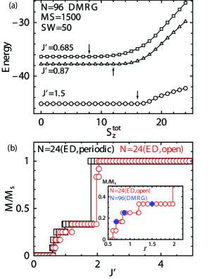
Figure 1: (Color) (a) Lowest energy in each subspace divided by $S_{z}^{\rm tot}$. Results of the DMRG calculations are presented when the size system is $N=96$ for $J^{\prime}=0.685,0.87$, and 1.5. Arrows indicate the spontaneous magnetization $M$ for a given $J^{\prime}$; $M$ is determined to be the highest $S_{z}^{\rm tot}$ among the values taking the lowest common energy. (b) $J^{\prime}$ dependence of the normalized magnetization $M/M_{\rm s}$ in the ground state. Red circles (black squares) denote the results obtained by ED calculations for a size system of $N=24$ under the open (periodic)-boundary condition. In the inset of (b), blue diamonds show the results obtained by DMRG calculations for a size system of $N=96$ under the open-boundary condition accompanied by red circles denoting the results obtained by ED calculations for a size system of $N=24$ under the open-boundary condition.

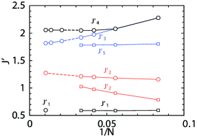
Figure 2: (Color) Size dependences of the phase boundaries. The results presented are those of $N=12,18,24$, and 30 from the ED calculations and those of $N=48,72$, and 96 from the DMRG calculations. Squares (circles) denote results in the cases under the periodic (open)-boundary condition. Dotted lines are drawn as guides for the eyes between the data from the ED and DMRG calculations. In the limit $N\rightarrow\infty$, the phase boundary between the $0<M/M_{\rm s}<1/3$ phase and the $M/M_{\rm s}=1/3$ phase seems to converge to approximately $J^{\prime}=1.30$.

First, let us examine the $J^{\prime}$ dependence of $M/M_{\rm s}$ to confirm the existence of the intermediate phase between the FM phase and the nonmagnetic DM phase irrespective of the boundary conditions, where $M_{\rm s}$ is the saturation value of the magnetization. Results are presented for $N=24$ from our ED calculations under the open and periodic boundary conditions in Fig. 1(b). We successfully observe the intermediate-magnetization phase irrespective of the boundary conditions. We also include in Fig. 1(b) some DMRG results of $N=96$, which suggests a weak size dependence of $M/M_{\rm s}$ as a function of $J^{\prime}$. Careful observation of the region of $0<M/M_{\rm s}\leq 1/3$ enables us to find that the intermediate-magnetization phase consists of two phases. One is the phase where $M/M_{\rm s}$ is fixed at $1/3$; this feature is that of the ferrimagnetism of the so-called Lieb-Mattis (LM) type, in which the spontaneous magnetization is fixed to be a simple fraction of the saturated magnetization[2, 3]. The other is the phase where $M/M_{\rm s}$ changes continuously with respect to the strength of $J^{\prime}$. This feature is certainly different from that of the LM ferrimagnetism; the continuous change in $M/M_{\rm s}$ is observed as the ferrimagnetism of the non-Lieb-Mattis (NLM) type in several models[15, 16, 17, 18, 19, 20, 21, 22]. We will determine later whether or not the phase of $0<M/M_{\rm s}<1/3$ in the present model is of the NLM type. Note here that these two phases are observed under both boundary conditions. On the other hand, the region of $1/3<M/M_{\rm s}<1$ is observed near $M/M_{\rm s}=1$ only under the open-boundary condition. At present, it is unclear whether or not this phase survives in the limit $N\rightarrow\infty$.

Next, we study the size dependences of the boundaries between the phases observed above. We investigate five boundaries: $J^{\prime}=J_{1}^{\prime}$ between the DM phase and the phase of $0<M/M_{\rm s}<1/3$, $J^{\prime}=J_{2}^{\prime}$ between the phase of $0<M/M_{\rm s}<1/3$ and the phase of $M/M_{\rm s}=1/3$, $J^{\prime}=J_{3}^{\prime}$ between the phase of $M/M_{\rm s}=1/3$ and the phase of $1/3<M/M_{\rm s}<1$, $J^{\prime}=J_{4}^{\prime}$ between the phase of $1/3<M/M_{\rm s}<1$ and the FM phase, and $J^{\prime}=J_{5}^{\prime}$ between the phase of $M/M_{\rm s}=1/3$ and the FM phase without the phase of $1/3<M/M_{\rm s}<1$. Note that $J^{\prime}_{3}$ and $J^{\prime}_{4}$ appear under the open-boundary condition, whereas $J^{\prime}_{5}$ appears under the periodic-boundary condition. Figure 2 shows the results of $N=12,18,24$, and 30 from the ED calculations and those of $N=48,72$, and 96 from the DMRG calculations. One finds that $J^{\prime}_{1}$ from the ED calculations under the periodic-boundary condition and that from the DMRG calculations under the open-boundary condition are consistent with each other; we have $J^{\prime}_{1}\sim 0.59$ as an extrapolated value. Concerning the boundary $J^{\prime}_{2}$, there exists a not so small difference between the result under the open-boundary condition and that under the periodic-boundary condition for a given $N$; however, $J^{\prime}_{2}$ seems to converge to 1.30 irrespective of the boundary condition. On the other hand, the situations of the boundaries of the phase of $M/M_{\rm s}=1/3$ and the FM phase are slightly complicated in our results. It seems that $J^{\prime}_{3}$ and $J^{\prime}_{4}$ become farther away from each other with increasing $N$ and that $J^{\prime}_{3}$ and $J^{\prime}_{5}$ converge to the same value of 1.77. We also have $J^{\prime}_{4}$ converging to 2.06. From these results of the extrapolation, it is evident that the phase of $M/M_{\rm s}=1/3$ and the phase of $0<M/M_{\rm s}<1/3$ exist in the thermodynamic limit. On the other hand, it is difficult to determine whether or not the phase of $1/3<M/M_{\rm s}<1$ is present. There is a possibility that this phase merges with the FM phase in the thermodynamic limit for two reasons: one is that this phase appears only near $M/M_{\rm s}=1$ and the other is that it is observed only under the open-boundary condition. The issue of whether or not this phase survives should be clarified in future studies; hereafter, we do not pay further attention to this phase.

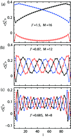
Figure 3: (Color) Local magnetization $\langle S_{i}^{z}\rangle$ under the open-boundary condition: (a) for $J^{\prime}=1.5$, (b) for $J^{\prime}=0.87$, and (c) for $J^{\prime}=0.685$ from the DMRG calculation for $N=96$. The site number is denoted by $i$, which is classified into $i=3n-2$, $3n-1$, and $3n$, where $n$ is an integer. Squares, circles, and triangles mean $i=3n-2$, $3n-1$, and $3n$, respectively.

Next, we examine the local magnetization $\langle S_{i}^{z}\rangle$ in the two phases of $0<M/M_{\rm s}<1/3$ and $M/M_{\rm s}=1/3$ to determine the magnetic properties in each phase. We present our DMRG results of $\langle S_{i}^{z}\rangle$ of the system of $N=96$. Note here that we calculate $\langle S_{i}^{z}\rangle$ within the subspace of the highest $S_{z}^{\rm tot}$ corresponding to the spontaneous magnetization $M$ obtained for a given $J^{\prime}$. The results of $\langle S_{i}^{z}\rangle$ are shown in Figs. 3(a)-3(c) for $J^{\prime}=0.685$, 0.87, and 1.5, respectively. In each case, one can observe a three-sublattice structure of the spin state clearly. In Fig. 3(a), the $i$ dependence of $\langle S_{i}^{z}\rangle$ in each of the sublattices of the spin structure is weak around the center of the system, although the edge effect spreads into a wide range from the edges. This behavior suggests that the spin state forms the LM ferrimagnetic state of up-up-down, which is consistent with $M/M_{\rm s}$=1/3 in the parameter region near approximately $J^{\prime}=1.5$. In Figs. 3(b) and 3(c), on the other hand, we find that the local magnetization shows a longer-distance periodicity in addition to the three-sublattice structure. The longer-distance periodicity changes when $J^{\prime}$ is changed within the phase of $0<M/M_{\rm s}<1/3$, the periodicity suggests an incommensurate modulation. A similar feature of this local structure was reported in some one-dimensional quantum frustrated spin systems[18, 19]. Therefore, the phase of $0<M/M_{\rm s}<1/3$ is considered as the NLM-type ferrimagnetic phase. This incommensurate feature originates from the effects of quantum fluctuation and frustration. We also calculate $\langle S_{i}^{z}\rangle$ for different system sizes, $N=48$ and 72. At least from these data (not shown in this papar), the periodicity and amplitude of the modulation seem to show only weak dependences on the system size. Note that the behavior of long-distance periodicity accompanied by the three-sublattice structure at the same time is different from the wave functions with a long periodicity reported in ref. References.

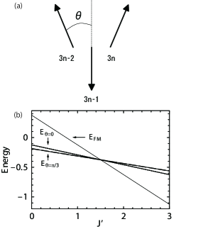
Figure 4: (a) Spin configuration from the point of view of classical vectors. The site number $i$ in the Hamiltonian (Frustration-Induced Ferrimagnetism in $S=1/2$ Heisenberg Spin Chain ) is classified into $3n$, $3n-1$, and $3n-2$, where $n$ is a positive integer. The angle $\theta$ for $J^{\prime}$ is determined by minimizing the classical energy. (b) $J^{\prime}$ dependences of classical energies of eq. (2) for $\theta=0$ (LM, dotted line), $\pi/3$ (NM, dotted chain line), and FM (solid line) energy of eq. (3).

Here, let us discuss the behavior of the intermediate phase between the FM phase and the nonmagnetic phase from the viewpoint that spins in the Hamiltonian (Frustration-Induced Ferrimagnetism in $S=1/2$ Heisenberg Spin Chain ) are assumed to be classical vectors. We consider the spin configuration of the classical vectors depicted in Fig. 4(a), where the characteristic angle $\theta$ is defined. This classical spin arrangement has been determined from our observation in Fig. 3 that the three-sublattice spin structure is realized in the intermediate region. The case of $\theta=0$ means that this classical state is the LM-type ferrimagnetic state with the ratio of the spontaneous magnetization to the saturated magnetization to be $1/3$. On the other hand, $\theta=\pi/3$ means that the state is in a nonmagnetic (NM) state. The classical energy per spin site under the periodic-boundary condition is given by

$$E(J^{\prime},\theta)=\frac{1}{24}[(6-4J^{\prime}){\rm cos}^{2}\theta-(6-4J^{\prime}){\rm cos}\theta+(-3-4J^{\prime})],$$ (2)

and the energy of the ferromagnetic state is given by

$$E_{\rm FM}=(3-4J^{\prime})/8.$$ (3)

The dependences of the energies shown in eqs. (2) and (3) are shown in Fig. 4(b). The FM (NM) phase appears at $J^{\prime}>1.5$ ($J^{\prime}<1.5$). One finds that $J^{\prime}$=1.5 is the boundary of the FM and NM phases. At exactly $J^{\prime}$=1.5, many states degenerate, including not only the FM and NM states but also the ferrimagnetic state with an arbitrary angle $\theta$. There is no intermediate phase between the two phases. It is worth emphasizing here that even the LM ferrimagnetic phase does not appear. This arguement suggests that the occurrence of the intermediate-magnetization state observed in the Hamiltonian (Frustration-Induced Ferrimagnetism in $S=1/2$ Heisenberg Spin Chain ) of the quantum system is a consequence of the quantum effect induced by frustration.

Finally, we mention another case when the intermediate-magnetization phase appears in the frustrated spin system in one dimension with anisotropic interactions[24, 25, 26, 27, 28]. Note here that this phase disappears in the isotropic case of interactions, which suggests that the origin of this phase is the anisotropy. However, it has not been examined yet whether or not this model shows a similar incommensurate modulation. Such examination would clarify the relationship between the intermediate magnetization of this model and the NLM ferrimagnetism studied in the present case.

In summary, we study the ground-state properties of an $S=1/2$ frustrated Heisenberg spin chain with isotropic interactions up to the fourth nearest neighbor by the ED and DMRG methods. In spite of the fact that this system consists of only a single spin site in each unit cell determined from the shape of the Hamiltonian, the ferrimagnetic ground state is surprisingly realized in a finite region between the ferromagnetic and nonmagnetic states. This result is in contrast to that of other systems of translationally invariant chains[29, 30]. We find that the intermediate region consists of phases of two ferrimagnetic types, the Lieb-Mattis type and non-Lieb-Mattis type. In the latter phase, we confirm that the local magnetization shows characteristic incommensurate modulation. The presence of the ferrimagnetic state without a sublattice structure of the shape of the system is a consequence of the strong quantum effect induced by frustration. Our findings shed light on a new aspect of the effect of frustration in quantum systems.

References

- [1] T. Sakai and K. Okamoto: Phys. Rev. B. 65 (2002) 214403.
- [2] E. Lieb and D. Mattis: J. Math. Phys. 3 (1962) 749.
- [3] W. Marshall: Proc. Roy. Soc. A 232 (1955) 48.
- [4] K. Takano, K. Kubo, and H. Sakamoto: J. Phys.: Condens. Matter 8 (1996) 6405.
- [5] K. Okamoto, T. Tonegawa, Y. Takahashi, and M. Kaburagi: J. Phys.: Condens. Matter 11 (1999) 10485.
- [6] T. Tonegawa, K. Okamoto, T. Hikihara, Y. Takahashi, and M. Kaburagi: J. Phys. Soc. Jpn. 69 (2000) Suppl. A, 332.
- [7] M. Ishii, H. Tanaka, M. Hori, H. Uekusa, Y. Ohashi, K. Tatani, Y. Narumi, and K. Kindo: J. Phys. Soc. Jpn. 69 (2000) 340.
- [8] As a candidate compound of the diamond chain system, natural mineral azurite, , is proposed[9, 10].
- [9] H. Kikuchi, Y. Fujii, M. Chiba, S. Mitsudo, and T. Idehara: Physica B 329-333 (2003) 967.
- [10] H. Ohta, S. Okubo, T. Kamikawa, T. Kunimoto, Y. Inagaki, H. Kikuchi, T. Saito, M. Azuma, and M. Takano: J. Phys. Soc. Jpn. 72 (2003) 2464-3467.
- [11] H. Nakano and M. Takahashi: J. Phys. Soc. Jpn. 66 (1997) 228.
- [12] C. K. Majumdar and D. K. Ghosh: J. Math. Phys. 10 (1969) 1399.
- [13] S. R. White: Phys. Rev. Lett. 69 (1992) 2863.
- [14] S. R. White: Phys. Rev. B. 48 (1993) 10345.
- [15] S. Sachdev and T. Senthil: Ann. Phys. 251 (1996) 76.
- [16] L. Bartosch, M. Kollar, and P. Kopietz: Phys. Rev. B 67 (2003) 092403.
- [17] N. B. Ivanov and J. Richter: Phys. Rev. B 69 (2004) 214420.
- [18] S. Yoshikawa and S. Miyashita: J. Phys. Soc. Jpn. 74 (2005) Suppl. 71.
- [19] K. Hida: J. Phys.: Condens. Matter 19 (2007) 145225.
- [20] K. Hida and K. Takano: Phys. Rev. B 78 (2008) 064407.
- [21] R. R. Montenegro-Filho and M. D. Coutinho-Filho: Phys. Rev. B 78 (2008) 014418.
- [22] H. Nakano, T. Shimokawa, and T. Sakai: submitted to J. Phys. Soc. Jpn.
- [23] J. Schulenburg and J. Richter: Phys. Rev. B 65 (2002) 054420
- [24] T. Tonegawa, I. Harada, and J. Igarashi: Prog. Theor. Phys. Suppl. 101 (1990) 513.
- [25] I. Harada and T. Tonegawa: J. Magn. Magn. Mater. 90 & 91 (1990) 234.
- [26] T. Tonegawa, H. Matsumoto, T. Hikihara, and M. Kaburagi: Can. J. Phys. 79 (2001) 1581.
- [27] T. Tonegawa and M. Kaburagi: J. Magn. Magn. Mater. 272-276 (2004) 898.
- [28] M. Kaburagi, T. Tonegawa, and M. Kang: J. Appl. Phys. 97 (2005) 10B306
- [29] T. Hamada, J. Kane, S. Nakagawa, and Y. Natsume: J. Phys. Soc. Jpn. 57 (1988) 1891
- [30] T. Tonegawa and I. Harada: J. Phys. Soc. Jpn. 58 (1989) 2902
- [31] A. F. Albuquerque, et al.: J. Magn. Magn. Mater. 310 (2007) 1187 (see also http://alps.comp-phys.org).