Anomalous diffusion in a symbolic model

Abstract

We address this work to investigate some statistical properties of symbolic sequences generated by a numerical procedure in which the symbols are repeated following a power law probability density. In this analysis, we consider that the sum of $n$ symbols represents the position of a particle in erratic movement. This approach revealed a rich diffusive scenario characterized by non-Gaussian distributions and, depending on the power law exponent and also on the procedure used to build the walker, we may have superdiffusion, subdiffusion or usual diffusion. Additionally, we use the continuous-time random walk framework to compare with the numerical data, finding a good agreement. Because of its simplicity and flexibility, this model can be a candidate to describe real systems governed by power laws probabilities densities.

I Introduction

The studies of complex systems are widespread among the physical communityAuyang ; hjj ; Barabasi ; Boccara and a large amount of these investigations deals with records of real numbers ordered in time or in space. Based on these time series, the aim of these works is to extract some features, patterns or laws which govern a given system. There is an extensive literature of statistical tools devoted to analyze time series. For instance, the detrended fluctuation analysis (DFA)Peng can be used to examine the presence of correlations in the data. However, many of these analysis are not focused on the original data but in sub-series like the absolute value, the return value or the volatility seriesMantegna .

In particular, a time series can be converted into a symbolic sequence by using a discrete partition in the data domain and assigning a symbol to each site of partition, technique that is known as symbol statisticsTang . A priori, any data set can be mapped into a symbolic sequence by using a specific rule (see for instance Ref. Steuer ). A typical analysis performed for this symbolic sequence is to evaluate its block entropy. This approach measures the amount of information contained in the block or the average information necessary to predict subsequent symbols. This analysis was applied to a wide range of topics, including DNA sequencesVoss . In this context, Buiatti et al.Buiatti introduced a numerical model which generates long-range correlations among the symbols of a symbolic sequence, leading to a slow growth of the usual block entropy.

Motivated by this anomalous behavior in the block entropy, our main goal is to construct a diffusive process based on these sequences. The diffusive processes generated with these sequences are expected to be Markovian or non-Markovian depending on the conditions imposed on these sequences. For Markovian processes or short-term memory systems the mean square displacement grows linearly in time. On the other hand, non-Markovian processes or long-term memory systems often display deviations of this linear behavior, being better described by a power law on time with the exponent $\alpha$. This is the fingerprint of the anomalous diffusion and depending on the $\alpha$ value we may have superdiffusion ($\alpha>1$) or subdiffusion ($\alpha<1$) and for $\alpha=1$ the usual spreading is recovered. Several physical systems exhibit this power law pattern. For instance, porous substratei1 , diffusion of high molecular weight polyisopropylacrylamide in nanoporesi2 , highly confined hard disk fluid mixturei3 , fluctuating particle fluxesi4 , diffusion on fractalsi5 , ferrofluidi6 , nanoporous materiali6a , and colloidsi7 .

In this context, the model proposed by Buiatti et al. has an essential ingredient leading to anomalous diffusion: the long-term memory present in their symbolic sequences. We will show that a diffusive process based on these sequences lead to a rich diffusive picture, where ballistic diffusion, superdiffusion, subdiffusion, and also usual diffusion can emerge, depending on the model parameters and on the mode of construction of the process. In addition, we compare our numerical results with analytic models based on continuous-time random walkMontroll ; Metzler ; Zumofen ; Klafter ; Gorenflo ; Gorenflo2 ; Barkai ; Meerschaert ; Zaburdaev ; Sololov .

This paper is organized as follows. In Section 2 we present and review some properties of the model. Section 3 is devoted to define erratic trajectories from the sequences as well as to investigate their diffusive behavior. A comparative analysis of this diffusive aspect with continuous-time random walk viewpoint is performed in Section 4. Finally, we end with a summary and some concluding comments.

II The model

The original modelBuiatti is a numerical experiment that generates equally likely symbols which are repeated among the sequence following a power law probability density. In order to describe the model, let $\mathcal{A}=\{a_{1},\dots,a_{n}\}$ be the set of symbols and $Q=\{Q_{1},Q_{2},\dots,Q_{N}\}$ represent a sequence where $Q_{i}\in\mathcal{A}$. To specify each $Q_{i}$, we initially select randomly one of the symbols of the alphabet $\mathcal{A}$ and repeated it $N_{y}$ times inside the sequence, in such way that $Q_{i}=Q_{i+1}=\dots=Q_{i+N_{y}-1}$. The number $N_{y}$ is obtained from

$$N_{y}=[y]+1\quad\mbox{with}\quad y=A\left[\frac{1}{(1-\eta)^{1/(\mu-1)}}-1\right]\,,$$ (1)

where $A>0$ and $\mu>1$ are real parameters, $\eta$ is a random variable uniformly distributed in the interval [0,1], and $[y]$ denotes the integer part of $y$. By using this procedure, a typical symbolic sequence with $N=10$ and $\mathcal{A}=\{-1,1\}$ is

$$Q=\left\{\underbrace{-1,-1,-1,}_{[y]+1=3}\underbrace{+1,+1,+1,+1,+1}_{[y]+1=5}\underbrace{-1,-1,}_{[y]+1=2}\right\}\,.$$

Since $\eta$ is a random number uniformly distributed, $y$ will be a positive random number. Moreover, $p(y)$ can be calculated in a straightforward manner leading to

$$p(y)=(\mu-1)\frac{A^{\mu-1}}{(A+y)^{\mu}}\;.$$ (2)

Therefore, the model basically consists in the repetitions of $N_{y}$ blocks of symbols with $N_{y}$ distributed according a power law of exponent $\mu$ in the asymptotic limit. Furthermore, the first and the second moments of $p(y)$ are given by

$$\langle y\rangle=\int_{0}^{\infty}\,y\,p(y)\,dy=\frac{A}{(\mu-2)}\,\;\mbox{(for $\mu>2$)}$$ (3)

and

$$\langle y^{2}\rangle=\int_{0}^{\infty}\,y^{2}\,p(y)\,dy=\frac{2A^{2}}{(\mu-2)(\mu-3)}\,\;\mbox{(for $\mu>3$).}$$ (4)

Note that when $\mu\leq 2$ both moments diverge and when $\mu\leq 3$ the second moment diverges while the first one remains finite. Thus, when $\mu$ is close to 2, $N_{y}$ can be very large filling a significante part of the sequence $Q$ with the same symbol. On the other hand, very large values of $N_{y}$ become rare for $\mu$ greater than 3 which makes the sequence highly alternating.

It is well established that this method of building symbolic sequences generates long-range correlations between elements of the sequence characterized by a power law correlation function (see the analytical development of Buiatti et al. Buiatti ). It was also studied that correlations lead to a non-linear growth of the usual block entropy, i.e., the usual entropy is not extensive for $\mu<3$. In such context, these sequences were investigated in the framework of the so called non-extensive Tsallis statistical mechanics. In particular, it was shown that the Tsallis block entropy $S_{q}$ can recover extensivity for a specific choice of the entropic index $q$Buiatti ; Ribeiro .

III Diffusive process

Figure 1: Erratic trajectories $x(n)$ for three values of $\mu$ when considering the two symbol alphabet $\mathcal{A}=\{-1,1\}$ and $A=1$. Note that depending on the values of $\mu$ the trajectories are very different.

As we raised in the introduction, long-term correlations or non-Markovian processes frequently present anomalous properties when investigated in the context of diffusion. In this direction, to construct erratic trajectories from these sequences may yield a rich diffusive scenario based on a simple model. This point has been noted by Buiatti et al. and also briefly discussed by us in Ref. Ribeiro .

A simple and direct way to obtain the trajectories is to consider that each symbol in a sequence represents the length of the jump of a particle in erratic movement. The position of the symbol plays the role of time. In this manner, the variable

$$x(n)=\sum_{i=1}^{n}Q_{i}\,$$ (5)

represents the position of the particle after a time $n$, which is an integer because of the construction.

Let us start our investigation by considering the simplest symmetric case, i.e., the two symbols alphabet $\mathcal{A}=\{-1,1\}$. Thus, the particle is equally likely to jump to the right or to the left according to whether $Q_{i}=1$ or $Q_{i}=-1$ and the variable $x(n)$ represents a random walk-like process where $x(1)=\pm 1$, $x(2)=0,\pm 2$, $x(3)=\pm 3,\pm 1$ and so on, with $n$ playing the role of time. Figure 1 illustrates $x(n)$ for three values of $\mu$ with $A=1$. Note that the trajectories are remarkably different depending on the values of $\mu$. For small values of $\mu$ ($\mu<3$), we can see that the trajectories are governed by two mechanisms: spatial localization and large jumps. When $\mu\leq 2$, larger is the jump, reflecting the fact that all moments of $p(y)$ diverge for $\mu\leq 2$. On the other hand, the second moment of $p(y)$ is finite for $\mu>3$ and the trajectories are very similar to usual random walks.

As pointed out in the introduction, when dealing with diffusive process, it is very common to investigate how the particles are spreading by evaluating the variance $\sigma^{2}(n)=\langle(x(n)-\langle x(n)\rangle)^{2}\rangle$, where the angle brackets denote an ensemble average. The usual Brownian motionGardiner ; Vlahos is characterized by $\sigma^{2}(n)\sim n$ and by a Gaussian propagator $p(x,n)\sim n^{-1/2}\exp(-x^{2}/2n)$ which is a direct consequence of the central limit theorem and the Markovian nature of the underlying stochastic process. On the other hand, the anomalous diffusion behavior is usually distinguished by the value of the exponent $\alpha$Dybiec in

$$\sigma^{2}(n)\propto n^{\alpha}\,.$$ (6)

We have subdiffusion when $0<\alpha<1$ and superdiffusion when $\alpha>1$. The crossover between subdiffusion and superdiffusion corresponds to the usual Brownian motion and the case $\alpha=2$ is the ballistic regime.

In this direction, we evaluate the variance for several values of $\mu$ over an ensemble average of $5\times 10^{5}$ realizations as shown in Figure 2a. In a log-log plot the slope of the curve $\sigma^{2}(n)$ versus $n$ is numerically equal to the exponent $\alpha$ which is visibly changing with the parameter $\mu$. In Figure 2b, we quantify this dependence by plotting $\alpha$ versus $\mu$. From this figure, we have basically three diffusion regimes depending on the existence of the first $\langle y\rangle$ and the second $\langle y^{2}\rangle$ moments of $p(y)$: (i) a ballistic one for $\mu<2$ ($\langle y\rangle\to\infty$ and $\langle y^{2}\rangle\to\infty$), (ii) a superdiffusive one for $2<\mu<3$ ($\langle y\rangle$ finite and $\langle y^{2}\rangle\to\infty$) and (iii) the usual Brownian motion for $\mu>3$ ($\langle y\rangle$ and $\langle y^{2}\rangle$ finite).

Figure 2: Results concerning the alphabet $\mathcal{A}=\{-1,1\}$ for $A=1$. (a) Logarithm of the variance $\sigma^{2}(n)$ versus logarithm of $n$ for $\mu=1.8$ (squares), $\mu=2.4$ (circles), $\mu=2.8$ (triangles) and $\mu=3.4$ (diamonds). In this figure, the slopes of the curves are numerically equal to the exponents $\alpha$ and the straight lines are linear fit to the data used to obtain the values of $\alpha$. (b) The dependence of the exponent $\alpha$ on $\mu$. From this figure, we have basically three diffusion regimes: a ballistic ($\mu\lesssim 2$), a superdiffusive ($2\lesssim\mu\lesssim 3$) and the usual Brownian motion ($\mu\gtrsim 3$). The straight lines are the predictions of the continuous-time random walk model related to equation (9).

Figure 3: (a) The dependence of the exponent $\alpha$ on $\mu$ when considering the alphabet $\mathcal{A}=\{-1,0,1\}$ and varying the probability of the zero symbol within the sequence. For the squares the symbols are equiprobable and for the circles the zero symbol is twenty times more likely to occur ($\mathcal{A}=\{-1,0^{20},1\}$). The triangles and the diamonds are the results concerning the larger alphabets $\mathcal{A}=\{-2,-1,0,1,2\}$ and $\mathcal{A}=\{-20,\dots,-2,-1,0,1,2,\dots,20\}$, respectively. (b) The dependence of the exponent $\alpha$ on $\mu_{z}$ when considering the equiprobable alphabet $\mathcal{A}=\{-1,0,1\}$ and $\mu_{j}=6$. Note the presence of a subdiffusive regime for $1\lesssim\mu_{z}\lesssim 2$. All results were obtained by using sequences of length $10^{7}$ averaged over $5\times 10^{5}$ realizations with $A=1$. The straight lines are the predictions of the continuous-time random walk model related to equation (9) and (10), respectively.

Next, we investigate the role of size of the symbol space by considering that more symbols are present in the alphabet $\mathcal{A}$. We consider first the presence of zeros, i.e., $\mathcal{A}=\{-1,0,1\}$ where each symbol is equiprobable within the sequence. The zero symbol allows the particles to stay motionless for a certain time what could be related to subdiffusion. However, as we show in Figure 3a the presence of zeros in the sequence does not significantly change the profile of the relation $\mu$ versus $\alpha$. Moreover, even if zero symbol becoming more probable within the sequence, i.e., $\mathcal{A}=\{-1,0^{T},1\}$ where $T$ is number of zero symbols in the alphabet, this result remains valid, as we also show in Figure 3a. Second, we study larger alphabets from $\mathcal{A}=\{-2,-1,0,1,2\}$ to $\mathcal{A}=\{-20,\dots,-2,-1,0,1,2,\dots,20\}$ and the results are shown in Figure 3a. We found that the relation $\mu$ versus $\alpha$ does not depend on the size of the symbol space. This relation is also robust for variations of the parameter $A$ and for non-symmetric alphabets. In particular, the parameter $A$ only produces a multiplicative effect in the equation (6) and a non-symmetric alphabet produces a drift which does not affect the spreading of the system.

Until now we were not able to generate subdiffusion, even adding the zero symbol more likely to occur. This result suggests that only superdiffusion can emerge when considering the same value of $\mu$ for the symbols that lead to jumps and for the zero symbol that lead to absence of motion. The reasons for this behavior are related to the fact that even the zero symbol being much more likely than other symbols, the number of repetitions $N_{y}$ is independent of the symbol. Thus, the particles can remain at rest for a long time but the flights can be equally long, since for $\mu<3$ there is no characteristic scale for $N_{y}$.

In this direction, let us consider a sequence where the jumping symbols are related to $\mu_{j}$ value ($\mu_{j}>3$) and the zero symbol is related other $\mu_{z}$ value. In this manner, the flights have a characteristic scale while the rest periods may or may not have this characteristic scale (depending on the $\mu_{z}$ value). The results concerning this scenario are shown in Figure  3b where we show the dependence of $\alpha$ on $\mu_{z}$ for a fixed value of $\mu_{j}=6$ (different values of $\mu_{j}>3$ does not affect this relation). From this figure, we can identify three diffusive regimes: no diffusion for $\mu_{z}\approx 1$ where the sequence is practically filled by zeros, subdiffusion $1\lesssim\mu_{z}\lesssim 2$ and usual diffusion for $\mu_{z}\gtrsim 2$.

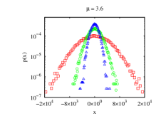
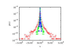
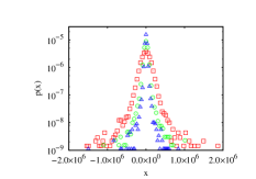
Figure 4: Probability density function of $x(n)$ for the values of $\mu$ (indicated in the figures) for three values of $n$ $10^{7}$ (squares), $2\times 10^{6}$ (circles) and $714\times 10^{3}$ (triangles), when considering the equiprobable alphabets $\mathcal{A}=\{-1,1\}$ (upper panel), $\mathcal{A}=\{-11,\dots,0,\dots 11\}$ (middle panel) and the alphabet $\mathcal{A}=\{-1,0^{10},1\}$ where the zero symbol is ten times more probable than the others (lower panel). The histograms were obtained by using sequences of length $10^{7}$ with $A=1$ and $5\times 10^{5}$ realizations of the numerical experiment.

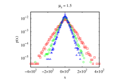
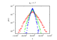
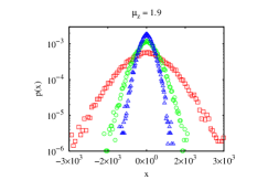
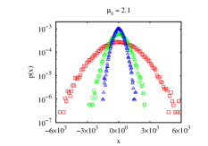
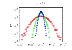
Figure 5: Probability density function of $x(n)$ for the values of $\mu_{z}$ (indicated in the figures) for three values of $n$ $10^{7}$ (squares), $2\times 10^{6}$ (circles) and $714\times 10^{3}$ (triangles). The histograms were obtained by using sequences of length $10^{7}$ with $A=1$, $\mu_{j}=6$ and $5\times 10^{5}$ realizations of the numerical experiment with the alphabet $\mathcal{A}=\{-1,0,1\}$.

We also evaluated the probability density functions (pdf) of $x(n)$ to investigate the shape of distribution $p(x,n)$ for different values of $\mu$ as well as for the different constructions of the erratic trajectories. Figure 4 shows these distributions for the equiprobable alphabets $\mathcal{A}=\{-1,1\}$ (upper panel), $\mathcal{A}=\{-11,\dots,0,\dots 11\}$ (middle panel) and the alphabet $\mathcal{A}=\{-1,0^{10},1\}$ with the zero symbol being ten times more probable than the others (lower panel). We can see that the distributions are characterized by non-Gaussian profiles with heavy tails when $\mu\lesssim 3$, recovering the Gaussian propagator when $\mu\gtrsim 3$. Further, a visual inspection suggests that the different constructions of the erratic trajectories only change the scale of these plots.

The situation is remarkably different when considering one value of $\mu$ for the jumping symbols and other for the zero symbol with the alphabet $\mathcal{A}=\{-1,0,1\}$. Figure 5 shows the distributions for this case. Notice that the shape of distributions goes from a Laplace ($p(x)\sim\exp(-|x|)$) to Gaussian distribution, depending on the $\mu_{z}$ value.

IV Continuous-time random walk models

So far we have empirically described the diffusive behavior of the symbolic sequences proposed by Buiatti et al.. Now let us compare these empirical findings with some analytical models based on continuous-time random walk.

In the continuous-time random walk (CTRW) of MontrollMontroll (see also Metzler ), the random walk process is fully specified by the function $\psi(x,t)$, the probability density to move a distance $x$ in time $t$. We can distinguish three different ways to make the movement: the particle waits until it moves instantaneously to a new position (jump model) or the particle moves at constant velocity to a new position and chooses randomly a new direction (velocity model) or the particle moves at constant velocity between turning points that are chosen randomlyZumofen . There are two fundamental approaches to the CTRW: (i) the decoupled and (ii) the coupled formalisms. In (i) the function $\psi(x,t)$ is supposed to factor in the form $\psi(x,t)=w(t)\lambda(x)$, i.e., the jumping and the waiting time are independent random variables. For (ii) both process are coupled, a jump of a certain length may involve a time cost or vice-versa. This coupled form commonly leads to more cumbersome calculations.

Here, we notice that because of the erratic trajectories construction, every continuous jump (without changing the sequence symbol) with length $N_{y}$ occurs at constant velocity and costs the same $N_{y}$ units of time to be performed. This fact lead us to the velocity and coupled model when considering the equiprobable alphabet $\mathcal{A}=\{-1,1\}$. When adding the zero symbol the resting times are decoupled from the jumps, but the jumping times stay coupled. In addition, we have to remember that our formal time $n$ is a discrete variable. Thus, comparisons with this formalism should be viewed as semi-quantitative. In this context, it is interesting to note that the work of Gorenflo et al.Gorenflo ; Gorenflo2 extends the Montroll’s theory to the discrete domain considering the decoupled version of the CTRW, in contrast to the first approach used here.

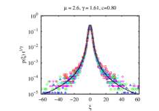
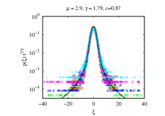
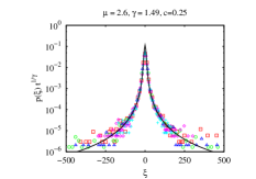
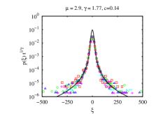
Figure 6: Probability density function of the scaling variable $\xi=c\,x/t^{\gamma}$ for some values of $\mu$ (indicated in the figure) for five values of $n$: $10^{7}$ (squares), $2\times 10^{6}$ (circles), $714\times 10^{3}$ (triangles), $55\times 10^{3}$ (diamonds) and $15\times 10^{3}$ (crosses). The upper panel shows the results for the equiprobable alphabet $\mathcal{A}=\{-1,1\}$, the middle panel for $\mathcal{A}=\{-11,\dots,0,\dots 11\}$ and the lower panel for $\mathcal{A}=\{-1,0^{10},1\}$ with the zero symbol been ten times more probable than the others. The continuous lines are the predictions of the the continuous-time random walk model, equation (11). The values of $c$ and $\gamma$ are indicated in the figure and the numerical data was obtained from $5\times 10^{5}$ realizations of equation (5) with $A=1$.

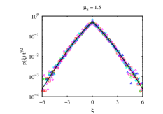
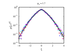
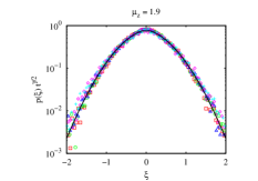
Figure 7: Probability density function of the scaling variable $\xi=cx/t^{\gamma/2}$ for some values of $\mu_{z}$ (indicated in the figure) for five values of $n$: $10^{7}$ (squares), $2\times 10^{6}$ (circles), $714\times 10^{3}$ (triangles), $55\times 10^{3}$ (diamonds) and $15\times 10^{3}$ (crosses) when considering the equiprobable alphabet $\mathcal{A}=\{-1,0,1\}$ and $\mu_{j}=6$. The continuous line is the prediction of the the continuous-time random walk model, equation (12) with $\gamma=0.47$ ($c=0.65$) for $\mu_{z}=1.5$, $\gamma=0.64$ ($c=0.37$) for $\mu_{z}=1.7$, $\gamma=0.94$ ($c=0.15$) for $\mu_{z}=1.9$. The numerical data was obtained from $5\times 10^{5}$ realizations of the numerical experiment with $A=1$.

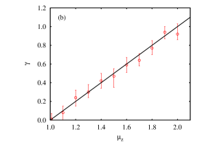
Figure 8: (a) The averaged value of $\gamma$ versus $\mu$ obtained via the procedure described in the text for the equiprobable alphabet $\mathcal{A}=\{-1,1\}$. (b) The averaged value of $\gamma$ versus $\mu_{z}$ when considering the equiprobable alphabet $\mathcal{A}=\{-1,0,1\}$ and $\mu_{j}=6$. Notice that the relation $\gamma=\mu-1$ or $\gamma=\mu_{z}-1$ obtained by comparing $w(t)$ and $p(y)$ is hold in general. The error bars are calculated via bootstrap resampling methodEfron .

Henceforth we start by considering the coupled velocity model of Zumofen and KlafterKlafter to compare with our sequences. For this case

$$\psi(x,t)=\frac{1}{2}\delta(|x|-t)\,w(t)\,,$$ (7)

where $w(t)\sim t^{-\gamma-1}$. Note that in this CTRW model long jumps are always penalized by long waiting times due to the presence of the $\delta$ function. Furthermore, because of the asymptotic behavior of $p(y)\sim y^{-\mu}$, $\gamma$ should be related to $\mu$ via $\gamma=\mu-1$. Now, following the approach of Zumofen and Klafter, we can write the form of the distribution $p(x,t)$ in the Fourier-Laplace space as

$$p(k,u)=\frac{\Psi(k,u)}{1-\psi(k,u)}\,,$$ (8)

where

$$\Psi(x,t)=\frac{1}{2}\delta(|x|-t)\int_{t}^{\infty}w(t^{\prime})dt^{\prime}$$

is the probability density to move a distance $x$ in time $t$ in a single event and not necessarily stop at $x$. By using $p(k,u)$, we can evaluate the variance

$$\sigma^{2}(t) = \mathcal{L}^{-1}\left[-\frac{\partial^{2}}{\partial k^{2}}p(k,u)\Bigl{|}_{k=0}\right]\sim\begin{cases}t^{2},&1<\mu<2,\\ t^{4-\mu},&2<\mu<3,\\ t,&\mu>3.\\ \end{cases}$$ (9)

Figure 2b shows the comparison with numerical data for the alphabet $\mathcal{A}=\{-1,1\}$ and Figure 3a makes this for the alphabets $\mathcal{A}=\{-1,0,1\}$ (with the zero symbol more probable) and also the larger alphabets $\mathcal{A}=\{-2,-1,0,1,2\}$ and $\mathcal{A}=\{-20,\dots,-2,-1,0,1,2,\dots,20\}$. Naturally, the agreement is better for the first case than the others, since it fulfills the requirements of the model. In general, we can see that the presence of the zero symbol makes the convergence of $\alpha$ to the limiting regimes slower($\alpha=2$ and $\alpha=1$).

We consider another CTRW model trying to reproduce the subdiffusive regime. Specifically, we employ the decoupled version proposed by MontrollMontroll2 where $\lambda(x)\sim\exp(-x^{2})$ and $w(t)\sim t^{-\gamma-1}$ ($0<\gamma<1$ ). Following MontrollMontroll2 or also Metzler and KlafterMetzler we obtain

$$\sigma^{2}(t)\sim t^{\mu_{z}-1}\,,$$ (10)

where again we have used the relation $\gamma=\mu_{z}-1$. Figure 3b confronts the numerical data with this expression for which we can see a good agreement.

Additionally, we may also obtain the propagator from a small $(k,u)$ expansion for both previous cases. For the first one $p(k,u)\sim 1/(u+c|k|^{\mu})$ which for $2<\mu<3$ yields

$$p(x,t)\sim\begin{cases}t^{-1/\gamma}L_{\gamma}(\xi),&|x|<t,\\ 0,&|x|>t,\end{cases}$$ (11)

where $L_{\gamma}(\xi)$ is the Lévy stable distribution and $\xi=c\,x/t^{\gamma}$ is the scaling variable. For the second one $p(k,u)\sim 1/(u+c\,k^{2}\,u^{\gamma})$ leading to

$$p(x,t)\sim t^{-\gamma/2}H_{1,2}^{2,0}\left[\xi^{2}|_{(0,1),(1/2,1)}^{(1-\gamma/2,\gamma)}\right]$$ (12)

where $H_{1,2}^{2,0}\left[\xi^{2}|_{(0,1),(1/2,1)}^{(1-\gamma/2,\gamma)}\right]$ is Fox $H$ function Fox and $\xi=cx/t^{\gamma/2}$ is the scaling variable.

Figure 6 shows the comparison for the first case and Figure 7 for the second one. In both cases we can see a good quality data collapse when the scaling is performed. Moreover, these figures show that we have found a good agreement between the numerical data and the CTRW models. The fitting parameter $\gamma$ of each case was obtained by minimizing the difference between the numerical data and the analytic expressions using the nonlinear least squares method. In all these figures we have employed the averaged value of $\gamma$ obtained from applying the method for 17 values of $n$ chosen logarithmically spaced from $10^{3}$ to $10^{7}$. In addition, Figures 8a and 8b show the dependence of the averaged value $\gamma$ on $\mu$ for both cases, showing that the relation $\gamma=\mu-1$ or $\gamma=\mu_{z}-1$ is consistent with the numerical data.

V Summary

Summing up, we verified that the symbolic model presented by Buiatti et al.Buiatti gives rise to a rich diffusive scenario. Depending on the parameter $\mu$ (or $\mu_{z}$), different anomalous diffusive regimes can emerge. Specifically, we have found subdiffusive, superdiffusive, ballistic, and usual regimes, depending on the model parameters and also on the trajectories construction. We also investigated the probability distributions of these processes where non-Gaussians were observed. Our findings support the existence of self-similarity in the data, due to the good quality of the data collapse when the scaling is performed. In addition, the numerical data were compared with predictions of the CTRW framework finding a good agreement. We believe that our empirical findings may help modeling systems for which power laws are present as well as to motivate other random walk constructions based on symbolic sequences.

- (1) S.Y. Auyang, Foundations of Complex-Systems (Cambridge University Press, Cambridge, 1998)
- (2) H.J. Jensen, Self-organized Criticality (Cambridge University Press, Cambridge, 1998)
- (3) R. Albert, A.-L. Barabási, Rev. Mod. Phys. 74, 47 (2002)
- (4) N. Boccara, Modeling complex systems (Springer-Verlag, New York, 2004)
- (5) C.-K. Peng et al., Nature 356, 168 (1992)
- (6) R.N. Mantegna, H.E. Stanley, An Introduction to Econophysics (Cambridge University Press, Cambridge, 1999)
- (7) X.Z. Tang, E.R. Tracy, R. Brow, Physica D 102, 253 (1997)
- (8) R. Steuer, L. Molgedey, W. Ebeling, M.A. Jiénez-Montaño, Eur. Phys. J. B 19, 265 (2001)
- (9) R.F. Voss, Phys. Rev. Lett. 68, 3805 (1992)
- (10) M. Buiatti, P. Grigolini, L. Palatella, Physica A 268, 214 (1999)
- (11) P. Brault et al., Phys. Rev. Lett. 102, 045901 (2009)
- (12) Y. Caspi, D. Zbaida, H. Cohen, M. Elbaum, Macromolecules 42, 760 (2009)
- (13) C.D. Ball, N.D. MacWilliam, J.K. Percus, R.K. Bowles, J. Chem. Phys. 130, 054504 (2009)
- (14) V.V. Saenko, Plasma Physics Reports 35, 1 (2009)
- (15) R. Metzler, G. Glockle, T.F. Nonnenmacher, Physica A 211 13 (1994)
- (16) A. Mertelj, L. Cmok, M. Copic, Phys. Rev. E 79, 041402 (2009)
- (17) R.M.A. Roque-Malherbe, Adsorption and Diffusion in Nanoporous Materials (Taylor and Francis Group, CCR Press, New York, 2007)
- (18) R. Golestanian, Phys. Rev. Lett. 102, 188305 (2009)
- (19) E.W. Montroll, G.H. Weiss, J. Math. Phys. 6, 167 (1965)
- (20) R. Metzler, J. Klafter, Physics Report 339, 1 (2000)
- (21) G. Zumofen, J. Klafter, Phys. Rev. E 47, 851 (1993)
- (22) G. Zumofen, J. Klafter, Europhys. Lett. 25, 565 (1994)
- (23) R. Gorenflo, A. Vivoli, Signal Processing 83, 2411 (2003)
- (24) R. Gorenflo, A. Vivoli, F. Mainardi, Nonlinear Dynamics 38, 101 (2004)
- (25) E. Barkai, Chemical Physics 284, 13 (2002)
- (26) M.M. Meerschaert, D.A. Benson, H.-P. Scheffler, P. Becker-Kern, Phys. Rev. E 66, 060102R (2002)
- (27) V.Y. Zaburdaev, K.V. Chukbar, J. Exp. Theor. Phys. 94, 252 (2002)
- (28) I.M. Sokolov, R. Metzler, Phys. Rev. E 67, 010101R (2003) (Springer, New York, 2009)
- (29) H.V. Ribeiro, E.K. Lenzi, R.S. Mendes, G.A. Mendes, L.R. da Silva, Braz. J. Phys. 39, 444 (2009)
- (30) C.W. Gardiner, Handbook of Stochastic Methods (Springer, Berlin, 2004).
- (31) L. Vlahos, H. Isliker, Y. Kominis, K. Hizanidis, arXiv:0805.0419v1 (2008).
- (32) B. Dybiec, E. Gudowska-Nowak, Phys. Rev. E 80, 061122 (2009).
- (33) E.W. Montrol, J. SIAM 4, 241 (1956)
- (34) A.M. Mathai, R.K. Saxena, The H-Function with Application in Statistics and Other Disciplines (Wiley Eastern, New Delhi, 1978)
- (35) B. Efron, R. Tibshirani, An Introduction to the Bootstrap (Chapman & Hall, London, 1993)