First principles calculations of anisotropic charge carrier mobilities in organic semiconductor crystals

Abstract

The orientational dependence of charge carrier mobilities in organic semiconductor crystals and the correlation with the crystal structure are investigated by means of quantum chemical first principles calculations combined with a model using hopping rates from Marcus theory. A master equation approach is presented which is numerically more efficient than the Monte Carlo method frequently applied in this context. Furthermore, it is shown that the widely used approach to calculate the mobility via the diffusion constant along with rate equations is not appropriate in many important cases. The calculations are compared with experimental data, showing good qualitative agreement for pentacene and rubrene. In addition, charge transport properties of core-fluorinated perylene bisimides are investigated.

I Introduction

Due to their low production costs and easy processability organic semiconductor devices are promising materials for organic light emitting diodes (OLEDs), Armstrong et al. (2009); Meerheim et al. (2009); Kulkarni et al. (2004) organic field effect transistors (OFETs), Dimitrakopoulos and Malenfant (2002); Newman et al. (2004); Facchetti (2007) radio frequency identification tags (RFIDs) Subramanian et al. (2005); Myny et al. (2010) and solar cells, Riede et al. (2008); Kippelen and Brédas (2009); Dennler et al. (2009); Chidichimo and Filippelli (2010); Deibel and Dyakonov (2010) to mention just a few. The performance of these devices depends crucially on the charge transport. Therefore, it is important to understand the basic principles of charge transport in these materials.

Various models have been proposed which are often contradictory. The band theory, which is well established for inorganic covalently bonded materials, is not particularly appropriate for organic conductors, because organic molecular crystals are only weakly bound by van der Waals interactions causing the molecules to be much more flexible. Due to the complex nodal structure of the molecular orbitals the transfer integrals between the monomers are very sensitive to even small nuclear displacements. That is why lattice vibrations play a more important role in organic than in inorganic materials, as they destroy the long range order and lead to a charge carrier localization. Brédas et al. (2009) To account for these vibrations, a variety of models have been proposed which incorporate the local (Holstein) Holstein (1959) and the nonlocal (Peierls) Peierls (1955) coupling. The latter leads to a polaron model where the charge carrier is partially localized and dressed by phonons. Hannewald et al. (2004); Hannewald and Bobbert (2004); Ortmann et al. (2010a, b) The fluctuations of the coupling between the molecules are of the same order of magnitude as the average coupling, Troisi et al. (2005) leading to a rather strong localization. Other models have been suggested, where the charges are assumed to be localized and the inter- and intramolecular vibrations are treated classically. Troisi and Orlandi (2006); Troisi (2007); Stafström (2010)

At higher temperatures, it is often appropriate to assume that the charge is localized due to the thermal disorder of the molecules and that charge transport occurs via thermally activated hopping. Schein et al. (1978) In some cases room temperature should be sufficient for this assumption to be justified. We apply this hopping model to study the dependence of the charge carrier mobility on the molecular structure and morphology as well as its angular dependency. The latter point is important since most organic crystals show a pronounced anisotropy for the transport parameters which has to be taken into account for device design. Furthermore, it is known that the mobility is very sensitive to the arrangement of the monomers and that already small changes in their alignment can alter the transport parameters dramatically. Brédas et al. (2002)

A promising class of materials for organic electronics are perylene bisimides. Due to their light resistance Herbst and Hunger (1997) and intense photoluminescence Langhals et al. (1998) they are widely used as robust organic dyes in the automobile industry. Herbst and Hunger (1997) Furthermore, they show a considerable electron mobility Struijk et al. (2000); Chen et al. (2004); An et al. (2005) and a high electron affinity. Schmidt et al. (2007); Chen et al. (2004) That is why they serve as n-type semiconductors for organic field effect transistors Chen et al. (2007); Schmidt et al. (2007); Weitz et al. (2008); Molinari et al. (2009); Wen et al. (2009a); Zhan et al. (2007) and as electron acceptor material in organic solar cells. Zhan et al. (2007); Wöhrle et al. (1995); Schmidt-Mende et al. (2001); Shin et al. (2006)

Section II describes the theoretical background of the applied model as well as details of the numerical calculations and computational approaches. It is shown that the master equation approach is particularly faster than the well-known Monte Carlo method. Furthermore we elucidate why the commonly applied approach to calculate the mobility via the diffusion constant along with rate equations Wen et al. (2009b); Liu et al. (2010); Deng and Goddard III (2004); Coropceanu et al. (2007) is not appropriate in many important cases. In Sec. III.1 we consider the frequently disputed question if the Einstein relation holds even for more disordered (amorphous) materials. Harada et al. (2005); Pautmeier et al. (1991); Borsenberger et al. (1991); Casado and Mejias (1994); Baranovskii et al. (1998a) In Sec. III.2 we show results for the orientational and morphological dependency of the mobility for pentacene, rubrene and two fluorinated perylene bisimides. The first two materials are experimentally and theoretically well investigated Mattheus et al. (2001); Malagoli et al. (2004); Jurchescu et al. (2004); Lee et al. (2006); Coropceanu et al. (2007); Wen et al. (2009b); Sundar et al. (2004); Podzorov et al. (2004); de Boer et al. (2004); da Silva Filho et al. (2005); Jurchescu et al. (2006); Zeis et al. (2006); Ling et al. (2007) which allows for the comparison with experimental data.

II Theory and modeling

II.1 The Marcus hopping model

In this work, a hopping mechanism is assumed for the motion of the charge carriers. The hopping rate from a site $i$ to $j$ is given by the Marcus equation Marcus (1956, 1993)

$$\nu_{ji}=\frac{{V_{ji}}^{2}}{\hbar}\sqrt{\frac{\pi}{\lambda k_{\mathrm{B}}T}}\exp\left[-\frac{(\Delta E_{ji}+\lambda)^{2}}{4\lambda k_{\mathrm{B}}T}\right],$$ (1)

where $V_{ji}$ is the electronic coupling parameter, $\lambda$ is the reorganization energy, $T$ is the temperature, $k_{\mathrm{B}}$ is the Boltzmann constant and $\hbar=h/(2\pi)$ where $h$ is the Planck constant. The energy difference $\Delta E_{ji}$ between the two hopping sites is caused by an external electric field $\vec{F}$. If the material is less ordered or even amorphous, each molecule experiences slightly different surrounding effects (such as polarization) that lead to different site energies $E_{i}^{0}$. These energy differences furthermore contribute to $\Delta E_{ji}$:

$$\Delta E_{ji}=(E_{j}^{0}-E_{i}^{0})-q\vec{F}\vec{r}_{ji},$$ (2)

where $q$ is the charge which equals the positive or negative unit charge and $\vec{r}_{ji}$ is the distance vector between sites $i$ and $j$. Marcus rates have been used before for calculating the anisotropy of the charge carrier mobility, Wen et al. (2009b) but with $\Delta E_{ji}\equiv 0$.

The interaction of the charge carriers with the phonons is partially considered by the reorganization energy. Due to the weak van der Waals interactions between organic molecules, it can be divided into an internal (intramolecular) and an external (intermolecular) part, i.e. $\lambda=\lambda_{\mathrm{int}}+\lambda_{\mathrm{ext}}$. The intramolecular reorganization energy $\lambda_{\mathrm{int}}$ is due to the geometry changes of the donor and the acceptor monomer upon the charge transfer process. The external reorganization energy $\lambda_{\mathrm{ext}}$ covers the energetic changes concerning the surrounding, caused by lattice distortion and polarization. For oligoacenes $\lambda_{\mathrm{ext}}$ was shown to be about one order of magnitude smaller than $\lambda_{\mathrm{int}}$. Norton and Brédas (2008); McMahon and Troisi (2010) Furthermore, is was demonstrated that $\lambda_{\mathrm{int}}$ of a molecule is lower in a cluster than in gas phase and that the total reorganization energy of naphthalene is closer to $\lambda_{\mathrm{int}}$ in the gas phase than to $\lambda_{\mathrm{int}}$ in the cluster. Norton and Brédas (2008) That is why the external reorganization energy is neglected in this paper and the internal reorganization energy of the monomer in vacuum is used for $\lambda$.

The Marcus theory was originally derived for outer sphere electron transfer in solvents. Marcus (1956) It stems from time dependent perturbation theory (Fermi’s Golden rule) and describes a non-adiabatic charge transfer where the charge carrier is localized at the donor or acceptor molecule respectively. Treating the coupling as a perturbation requires that $V_{ji}$ is small compared to $\lambda/4$, which corresponds to the activation energy for the charge carrier to change place (for $\Delta E_{ji}=0$). Furthermore, the thermal relaxation (the geometric reorganization) has to be fast in comparison with the transfer so that the system can be assumed to be in thermal equilibrium during the transfer. In addition, the theory is restricted to the high temperature case since tunneling is neglected completely and the molecular vibrations are treated classically, what requires $k_{\mathrm{B}}T\gg\hbar\omega$. These restrictions of the Marcus theory in the context of charge transport are discussed elsewhere. Picon et al. (2007); Cheung and Troisi (2008) Despite all imperfections it is widely used for charge transfer in organic crystals Deng and Goddard III (2004); Li et al. (2007); Wen et al. (2009b); Liu et al. (2010); Sancho-García and Pérez-Jiménez (2008); Sancho-García et al. (2010); Sancho-García and Pérez-Jiménez (2009) and one can certainly assume that this theory is suitable for the purpose of a qualitative charge transport analysis.

II.2 The master equation approach

The master equation approach was used to describe the transport process. In the case of low charge carrier densities, the master equation, which describes the hopping of the charge carriers in the organic semiconductor, has the simple linear form Houili et al. (2006)

$$\frac{dp_{i}}{dt}=\sum_{j}(\nu_{ij}p_{j}-\nu_{ji}p_{i}),$$ (3)

where $p_{i}$ denotes the probability that the lattice site $i$ is occupied by a charge carrier. The index $j$ sums over all other sites. In principle, it is also possible to include repulsive forces between the charge carriers in the master equation in order to account for higher charge carrier densities. However, in the case of low densities, even the quite simple Eq. (3) leads to good results.

In the steady state, a dynamic balance is reached where the occupation probabilities for the sites do not change anymore and $dp_{i}/dt$ in Eq. (3) equals zero. Since this equation holds for all sites in the crystal, this results in a linear system of equations,

$$\mathbf{N}\cdot\vec{p}=\vec{0}.$$ (4)

$\vec{p}$ contains the unknown $p_{i}$ and $\mathbf{N}$ is a negative semidefinite sparse matrix that contains all hopping rates $\nu_{ji}$. For one dimension $\mathbf{N}$ is

$$\left(\begin{array}[]{c|cccc|c}&\vdots&\vdots&\vdots&\vdots&\\ \hline\cr\ldots&-\sum_{j}\nu_{j1}&\nu_{12}&\nu_{13}&\nu_{14}&\ldots\\ \ldots&\nu_{21}&-\sum_{j}\nu_{j2}&\nu_{23}&\nu_{24}&\ldots\\ \ldots&\nu_{31}&\nu_{32}&-\sum_{j}\nu_{j3}&\nu_{34}&\ldots\\ \ldots&\nu_{41}&\nu_{42}&\nu_{43}&-\sum_{j}\nu_{j4}&\ldots\\ \hline\cr&\vdots&\vdots&\vdots&\vdots&\end{array}\right).$$ (5)

The columns correspond to the initial sites $i$ of the charge carrier and the lines correspond to the final sites $j$, i.e., the jump rate $\nu_{ji}$ from $i$ to $j$ appears in the $i$th column and the $j$th line. The diagonal elements contain the negative sum of all hopping rates away from the respective site.

The infinite matrix $\mathbf{N}$ is approximated by a finite matrix with cyclic boundary conditions, i.e., a charge carrier that leaves the crystal at one side reenters at the opposite side. This means for the example matrix depicted in Eq. (5) that the charge which jumps from site 4 in positive direction ends at site 1. For this boundary condition to be applicable it has to be assured that the hopping rate from site 4 to site 1 in negative direction is negligible. This results in a constraint for the minimum size of the matrix.

The matrix in Eq. (5) was extended to three dimensions resulting in a $(3n_{d}n_{m})\times(3n_{d}n_{m})$ matrix where $n_{d}$ is the number of unit cells in each direction and $n_{m}$ is the number of monomers per unit cell. In this work all monomers within a cube of three unit cells length in each dimension of the crystal are taken into account. It was verified that a bigger matrix with more than $3\times 3\times 3$ unit cells does not change the result. The hopping rates were calculated from one monomer to all other monomers in the same and in the adjacent cells. Since the jump rate, Eq. (1), implicitly depends on the distance via the electronic coupling $V_{ji}$, larger jump distances can be neglected.

Solving Eq. (4) and taking into account the normalization condition $\sum_{i}p_{i}=1$ provides the occupation probabilities for all sites. (For $\Delta E_{ji}=0$, it is the same for all sites.) These probabilities can then be used to calculate the mobility of the charge carriers in field direction from

$$\mu=\frac{\langle v\rangle}{F},$$ (6)

with the average velocity

$$\langle v\rangle=\sum_{i}p_{i}v_{i}=\sum_{i}p_{i}\frac{\langle r_{\parallel}\rangle_{i}}{\tau_{i}},$$ (7)

where $v_{i}$ is the resulting velocity at site $i$,

$$\langle r_{\parallel}\rangle_{i}=\frac{\sum_{j}\nu_{ji}\left(\vec{r}_{ji}\frac{\vec{F}}{F}\right)}{\sum_{j}\nu_{ji}}$$ (8)

is the average displacement at site $i$ in field direction and

$$\tau_{i}=\left(\sum_{j}\nu_{ji}\right)^{-1}$$ (9)

is the dwell time of the charge carrier at site $i$. Equations (6) to (9) result in Yu et al. (2001)

$$\mu = \frac{1}{F}\sum_{i}\left(p_{i}\sum_{j}\nu_{ji}\frac{\sum_{j}\nu_{ji}\left(\vec{r}_{ji}\frac{\vec{F}}{F}\right)}{\sum_{j}\nu_{ji}}\right)$$ (10)

$$= \frac{1}{F}\sum_{ij}p_{i}\nu_{ji}\vec{r}_{ji}\frac{\vec{F}}{F}.$$

In order to simplify the calculation of the mobility within such a jump rate approach, the mobility is often calculated without external field because the occupation probabilities of the sites do not differ in this case and one does not have to solve the master equation (4). Since Eq. (10) is not applicable in that case (because $F=0$), the mobility is calculated via the diffusion coefficient $D$ and the Einstein relation Landsberg (1981)

$$\mu=\frac{q}{k_{\mathrm{B}}T}D.$$ (11)

Different equations are found in the literature Wen et al. (2009b); Deng and Goddard III (2004); Liu et al. (2010); Coropceanu et al. (2007); Bisquert (2008) to evaluate $D$. Considerations similar to those above for the mobility seem to provide

$$D=\frac{1}{2n}\frac{d}{dt}\langle r^{2}\rangle=\frac{1}{2n}\sum_{i}p_{i}\frac{\langle r^{2}\rangle_{i}}{\tau_{i}},$$ (12)

where $n$ is the spatial dimensionality. Since the diffusion is regarded in one dimension here, $n$ equals 1 and

$$D=\frac{1}{2}\sum_{i}p_{i}\frac{\langle r^{2}_{\parallel}\rangle_{i}}{\tau_{i}},$$ (13)

where

$$\langle r^{2}_{\parallel}\rangle_{i}=\frac{\sum_{j}\nu_{ji}(\vec{r}_{ji}\vec{e})^{2}}{\sum_{j}\nu_{ji}}$$ (14)

is the variance of the charge carrier position at site $i$ in the direction of the unit vector $\vec{e}$. Equations (9) and (12) to (14) finally result in

$$D=\frac{1}{2}\sum_{ij}p_{i}\nu_{ji}\left(\vec{r}_{ji}\vec{e}\right)^{2}$$ (15)

for the diffusion coefficient in the direction of $\vec{e}$. It is worth mentioning that Eq. (15) holds even in the presence of an external field (see Appendix A).

Without external field and assuming that all lattice sites are equal (i.e. $\Delta E_{ji}=0$), the last equation simplifies to Coropceanu et al. (2007); Zhdanov (1985); Myshlyavtsev et al. (1995)

$$D=\frac{1}{2}\sum_{j}\nu_{j}(\vec{r}_{j}\vec{e})^{2}.$$ (16)

It is important to note, that the diffusion constants in Eqs. (15) and (16) are not strictly correct. Just if the unit cell of the crystal contains only a single molecule and if the crystal structure is perfectly translation-symmetric, i.e. $E_{i}^{0}=E_{j}^{0}$ for all monomer pairs, cf. Eq. (2), these equations become correct.

However, in less ordered or even amorphous materials the site energies $E_{i}^{0}$ and $E_{j}^{0}$ are different because of the differing surroundings for each lattice site. In that case, the occupation probabilities $p_{i}$ differ and the master equation has to be applied. In the case of strongly different $E_{i}^{0}$, even Eq. (15) becomes incorrect since the charge carrier can be “trapped” between two lattice sites with similar energy, Gonzalez-Vazquez et al. (2009) see Fig. 1a: Because of the energetically unfavorable surrounding, the charge carrier jumps back and forth between the same sites all the time. These moves do not contribute to a macroscopic spreading of the occupation probability of the charge carrier with the time. That is why the averaging in Eq. (15) overestimates the true macroscopic diffusion coefficient. This problem does not appear in Eq. (10) since the $\vec{r}_{ji}$ is not squared as in Eq. (15). For that reason the contribution of the trapped charge cancels when summing over all lattice sites. And even in perfectly ordered crystals where all jump rates are symmetric, i.e. $\nu_{ji}=\nu_{ij}$ (without external field), such a trapping can occur if different sites exist in the elementary cell of the crystal and if the hopping rates within the cells differ from those to neighbored unit cells, see Fig. 1b: Here, the charge carrier jumps back and forth between two monomers with a high coupling because the coupling to the other neighbors is lower. In such cases Eq. (10) in conjunction with Eq. (11) provides correct diffusion coefficients while Eqs. (15) and (16) overestimate the values for $D$.

Figure 1: The charge carrier is “trapped” between two lattice sites. a) The surrounding of the monomer causes an energetic “pit”. b) Strongly differing jump rates lead to a capturing.

II.3 The Monte Carlo approach

The master equation results were verified with Monte Carlo simulations applying the algorithm of Houili et al., Houili et al. (2006) but without any interaction between the charge carriers. The mobility and the diffusion coefficient were calculated via

$$\mu=\frac{1}{F}\frac{d}{dt}\left\langle\vec{r}_{ji}\frac{\vec{F}}{F}\right\rangle$$ (17)

and

$$D=\frac{1}{2}\frac{d}{dt}\left\langle\left(\vec{r}_{ji}\vec{e}-\left\langle\vec{r}_{ji}\vec{e}\right\rangle\right)^{2}\right\rangle$$ (18)

respectively. The time dependent average position $\langle\vec{r}_{ji}\frac{\vec{F}}{F}\rangle$ and the variance $\langle\left(\vec{r}_{ji}\vec{e}-\left\langle\vec{r}_{ji}\vec{e}\right\rangle\right)^{2}\rangle$ have been averaged over a sufficient number of simulation runs to obtain smooth lines. It was checked that both average and variance show a linear time dependence in order to secure the stationary state.

The Monte Carlo approach is just an alternative way to solve the master equation (3). It is a feasible way to log the atomic scale motions underlying the transport properties as a function of time. However, as this is a stochastic method, many simulation runs are needed in order to achieve an acceptably low statistical error such that sufficiently significant values are obtained for the mobility and the diffusion coefficient. Furthermore, one has to take care that the stationary state is reached within the simulation time. This is a serious problem in the case of strongly disordered materials. In contrast to that, the approach used here by solving the matrix equation (4) which provides the stationary state by means of analytic numerical methods guarantees the stationary solution and is furthermore numerically more efficient than Monte Carlo simulations. Yu et al. (2001)

II.4 Quantum chemical methods

The electronic coupling $V_{ji}$ and the reorganization energy $\lambda$ needed for the hopping rate, Eq. (1), are determined by quantum chemical first principles calculations. In order to calculate $\lambda$, the geometry of the isolated monomer was optimized for the charged and the neutral state. The energies $E_{0}$ and $E_{c}$ of the neutral and the charged monomers in their lowest energy geometries and the energies $E_{0}^{*}$ and $E_{c}^{*}$ of the neutral monomer with the ion geometry and the charged monomer with the geometry of the neutral state are calculated to get the intramolecular reorganization energy Malagoli et al. (2004)

$$\lambda=\lambda_{c}+\lambda_{0}=(E_{c}^{*}-E_{c})+(E_{0}^{*}-E_{0}),$$ (19)

cf. Fig. 2. For all quantum chemical calculations the TURBOMOLE program package tur (2009) was used. The calculations were conducted via density functional theory using the hybrid generalized gradient functional B3-LYP Dirac (1929); Slater (1951); Vosko et al. (1980); Becke (1988); Lee et al. (1988); Becke (1993) with the correlation consistent polarized valence double zeta basis set (cc-pVDZ) Dunning (1989) for all atoms. This functional was chosen because it has been shown that it leads to quite good results for describing the ionization-induced geometry modifications of oligoacenes. Sánchez-Carrera et al. (2006); Coropceanu et al. (2002)

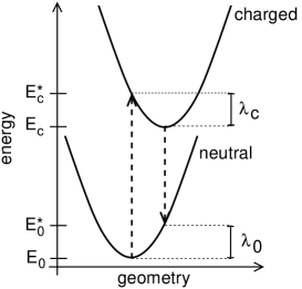
Figure 2: The potential energy surfaces of the neutral and the charged monomer. The dashed arrows indicate the vertical transitions from one state to the other. $\lambda_{0}$ and $\lambda_{c}$ are the two contributions to the reorganization energy, see Eq. (19).

The electronic couplings were calculated as described by Li et al. Li et al. (2007) resulting in

$$V_{ji}=\frac{H_{ji}-\frac{1}{2}(H_{ii}+H_{jj})S_{ji}}{1-S_{ji}^{2}}$$ (20)

with

$$H_{ji} = \langle\varphi_{j}|\hat{H}_{KS}|\varphi_{i}\rangle$$

$$S_{ji} = \langle\varphi_{j}|\varphi_{i}\rangle.$$

For hole (electron) transport $\varphi_{i}$ and $\varphi_{j}$ are the HOMO (LUMO) orbitals of the respective isolated monomers and $\hat{H}_{KS}$ is the Kohn-Sham operator of the neutral dimer system. $H_{ii}$ and $H_{jj}$ are the site energies of the two monomers, $S_{ji}$ is the spatial overlap and $H_{ji}$ is the charge transfer integral in the non-orthogonalized basis.

The arrangement of the monomers in the crystal was extracted from X-ray crystal structure data which was retrieved from the Cambridge Structural Database.

II.5 The Gaussian disorder model

It has been argued that the Einstein relation, Eq. (11), does not hold in disordered organic materials in general Pautmeier et al. (1991); Borsenberger et al. (1991); Casado and Mejias (1994) or at least if additionally an external field is applied. Bisquert (2008); Anta et al. (2008); Novikov and Malliaras (2006) In fact it turned out that this is only true for rather high charge carrier densities, Roichman and Tessler (2002) low temperatures and high electric fields which are out of the scope of the present work. At extremely low temperatures, the thermal energy of the charge carriers is not sufficient to reach sites which are higher in energy and only energy-loss jumps occur. In that case, neither $\mu$ nor $D$ depends on the temperature. Baranovskii et al. (1998b) For low fields, the transport coefficients are independent of the field, Abkowitz et al. (1991); Bässler (1993) but for higher fields nonlinear effects become important and $D/\mu$ increases with increasing field. Richert et al. (1989)

A strongly disordered organic semiconductor was simulated by means of the Gaussian disorder model Bässler (1993) with a Gaussian shaped density of states,

$$\varrho(E)=\frac{1}{\sqrt{2\pi\sigma^{2}}}\exp\left(-\frac{E^{2}}{2\sigma^{2}}\right),$$ (21)

where the standard deviation $\sigma$ is called the energetic disorder of the simulated material, in conjunction with the Miller-Abrahams jump rate Miller and Abrahams (1960)

$$\nu_{ji} = \nu_{0}\exp(-2\gamma r_{ji})\times$$ (25)

$$\left\{\begin{array}[]{ll}\exp\left(-\frac{\Delta E_{ji}}{k_{\mathrm{B}}T}\right),&\Delta E_{ji}\geq 0\\ 1,&\Delta E_{ji}<0\end{array}\right.$$

where $\nu_{0}=10^{13}$ s^-1 is the attempt-to-jump frequency and $\gamma=5\cdot 10^{9}$ m^-1 is the inverse localization radius. The first exponential function describes the tunneling of the charge and the Boltzmann-type exponential function accounts for thermally activated jumps upwards in energy. Hops to lower energies are not thermally activated.

A simple cubic lattice of sites with a lattice constant of 1 nm was used. In order to achieve a sufficient statistics for the site energies the lattice consisted of $80\times 40\times 40$ sites. For a given site only the hops from and to the 26 adjacent sites were considered. Calculations with a bigger lattice and also further jump targets taken into account did not affect the result.

III Results and discussion

III.1 Validity of the Einstein relation

The mobility and the diffusion coefficient were calculated by the master equation approach in conjunction with the Eqs. (10) and (15) and by the Monte Carlo approach using Eqs. (17) and (18) respectively. The Gaussian disorder model described in Sec. II.5 was used. In the Monte Carlo simulation, the average and the variance of the charge carrier position has been averaged over 50.000 trajectories and the simulation time has been up to 1 s.

Figure 3 shows the results as a function of the energetic disorder $\sigma$, cf. Eq. (21). The mobility varies over several orders of magnitude and the results of Eqs. (10) and (17) match exactly. This is not the case for the diffusion coefficient calculated with Eq. (15) and (18). With increasing energetic disorder, the deviations between these two approaches to calculate $D$ increase. These deviations are not caused by the field because for $\sigma=0$ the results match. In order to decide which one is the right approach, the ratio $D/\mu$ is plotted as well. One clearly sees that in the case of Monte Carlo the Einstein relation, Eq. (11), is valid, whereas $D/\mu$ calculated with Eqs. (15) and (10) deviates from the Einstein relation. The two mobility equations lead to the same results. Thus, Eq. (15) and also the frequently used Eq. (16) provide incorrect diffusion constants for energetically inhomogeneous materials. In any case it is advantageous to employ the master equation in conjunction with Eq. (10) to calculate the mobility as this provides correct diffusion constants without numerical noise and with low computational demands.

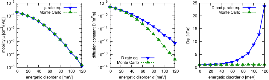
Figure 3: (Color online) Mobility, $\mu$, (left) diffusion coefficient, $D$, (middle) and the ratio $D/\mu$ (right) as a function of the energetic disorder, calculated with the rate equations (10) and (15) respectively, and via Monte Carlo simulation. The calculations were conducted at $T$ = 300 K and $F=10^{5}$ V/m.

III.2 Angular dependence of the mobility in crystals

If not otherwise stated, the calculations have been conducted with an electric field of $10^{7}$ V/m and a temperature of 300 K. The molecules under investigation are depicted in Fig. 4 and the crystallographic parameters of the corresponding crystals are listed in Tab. 1.

Figure 4: The molecules investigated in this work: a) pentacene, b) rubrene, c) PBI-F₂, d) PBI-(C₄F₉)₂.

Table 1: Lattice constants and angles for the unit cells of all calculated crystals.

	a [Å]	b [Å]	c [Å]	$\alpha$ [∘]	$\beta$ [∘]	$\gamma$ [∘]	Ref.
pentacene	6.27	7.78	14.53	76.48	87.68	84.68	Mattheus et al.,2001
rubrene	26.86	7.19	14.43	90.00	90.00	90.00	Jurchescu et al.,2006
PBI-F2	17.46	5.28	15.28	90.00	110.90	90.00	Schmidt et al.,2007
PBI-(C4F9)2	10.57	12.89	16.68	66.86	76.52	84.62	Li et al.,2008

III.2.1 Pentacene

Pentacene (see Fig. 4a) exists in several morphologies. Here the structure described by Mattheus et al. Mattheus et al. (2001) (at 293 K) was investigated. The unit cell contains two differently orientated monomers. Pentacene is known to be a hole conductor, but for comparison, the electron transport is regarded here as well. The reorganization energy was calculated to 92 meV for holes and 131 meV for electrons. This is in good agreement with values reported before (98 and 95 meV for holes Coropceanu et al. (2007); Malagoli et al. (2004) and 132 meV for electrons. Coropceanu et al. (2007))

Figure 5 shows the mobilities of holes and electrons in the crystal in all three dimensions. For better legibility Fig. 6 shows two dimensional cross sections orthogonal to the $a^{*}$, $b^{*}$ and $c^{*}$ direction respectively. The magnitudes of the hole and electron mobility are quite similar. For both types of charge carriers the transport is almost two dimensional since the minimal mobility, that is found in the $c^{*}$ direction, is very low (0.2 cm²/V s for holes and 1.3 cm²/V s for electrons) compared with the other directions. This can be explained by the electronic couplings. The highest ones are listed in Tab. 2. The directions of the corresponding charge transitions are drawn in Fig. 7. All of them are coplanar in the $ab$ plane. For holes, the biggest coupling belonging to a transition with a component in $c$ direction is one order of magnitude lower than the lowest coupling listed in Tab. 2 (electrons: about factor 5 smaller). The highest couplings for holes belong to the transitions in [11̄0] direction, the second highest to the [110] direction. The reverse is true for electrons. That is why the directionality of the mobilities for holes and electrons differ in the $ab$ plane. The maximum mobility for holes (18.5 cm²/V s) is found at $132^{\circ}$, the maximum for electrons (13.7 cm²/V s) at $37^{\circ}$.

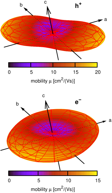
Figure 5: (Color online) The mobility for holes (top) and electrons (bottom) in the pentacene crystal for $F=10^{7}$ V/m and $T=300$ K.

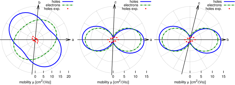
Figure 6: (Color online) The mobility for holes and electrons in the pentacene crystal in the $ab$ plane (left), $ac$ plane (middle) and $bc$ plane (right). The parameters are the same as in Fig. 5. For comparison some experimental values Lee et al. (2006) are plotted. Note that in the experiment the crystal orientation could not be determined Lee et al. (2006) and therefore the experimental data is rotated to fit best.

Table 2: The most important electronic couplings and the reorganization energy in the pentacene crystal for electrons and holes, cf. Fig. 7.

	$h^{+}$ [meV]	$e^{-}$ [meV]
$V_{1}$	90.69	85.18
$V_{2}$	55.05	89.66
$V_{3}$	39.68	50.00
$V_{4}$	36.62	47.10
$\lambda$	92	131

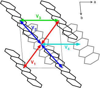
Figure 7: (Color online) The most important hopping paths in the pentacene crystal. Direction of view is parallel to the $c^{*}$ axis.

Figure 6 shows a comparison between the calculation and some experimental mobility values for holes. Lee et al. (2006) Please note, that the crystal orientation could not be determined in the experiment. Lee et al. (2006) The measured mobility varies between 0.66 and 2.3 cm²/V s. This shows that the calculated maximal mobility is almost one order of magnitude too big. However, in highly purified single crystals of pentacene a mobility of 35 cm²/V s has been measured. Jurchescu et al. (2004) It was also experimentally confirmed that the mobility in the $ab$ plane is much larger than along the $c^{*}$ axis. Jurchescu et al. (2004) This is in agreement with our calculations where the minimal mobility of about 0.2 cm²/V s is in $c^{*}$ direction. For room temperature and lower, the measurements showed a temperature dependence of the mobility following $\mu\propto T^{-n}$ with a positive $n$ indicating band transport. Jurchescu et al. (2004) While this is not in accordance with the thermally activated hopping model used here, it was also shown that above room temperature a different transport mechanism dominates the mobility. A further reason for the overestimation of the mobility is that the nonlocal electron-phonon couplingHannewald et al. (2004); Hannewald and Bobbert (2004); Ortmann et al. (2010a, b); Troisi et al. (2005); Troisi and Orlandi (2006); Troisi (2007); Stafström (2010) is neglected in our model. While the absolute values do not match the measured mobilities, the qualitative dependency on the crystal direction fits to the experimental results.

III.2.2 Rubrene

Rubrene (see Fig. 4b) is a hole conductor. It crystallizes with four differently oriented monomers in the unit cell. The calculations were conducted using the morphology described by Jurchescu et al. Jurchescu et al. (2006) at 293 K. Table 3 shows the reorganization energies and the values of the four highest electronic couplings. The couplings next in size are two orders of magnitude smaller than the smallest coupling listed. This is in agreement with previous calculations. Wen et al. (2009b); Coropceanu et al. (2007) The hopping paths corresponding to these couplings are drawn in Fig. 8. The largest coupling ($V_{1}$) is between equally oriented monomers along the $b$ direction, which is the smallest lattice constant. The second largest couplings are between monomers which lie in the same plane perpendicular to the $a$ axis. $V_{3}$ is the coupling between these planes and $V_{4}$ is the coupling between monomers in the same plane perpendicular to the $b$ axis.

Table 3: The most important electronic couplings and the reorganization energy in the rubrene crystal for holes and electrons, cf. Fig. 8. For comparison calculated values for holes from Refs. Wen et al., 2009b and Coropceanu et al., 2007 are shown.

	$h^{+}$ [meV]	$e^{-}$ [meV]	$h^{+}$ [meV] Wen et al. (2009b)	$h^{+}$ [meV] Coropceanu et al. (2007)
$V_{1}$	95.73	49.40	89	83
$V_{2}$	16.38	5.55	19	15
$V_{3}$	1.36	0.59
$V_{4}$	0.24	0.24
$\lambda$	146	199	152	159

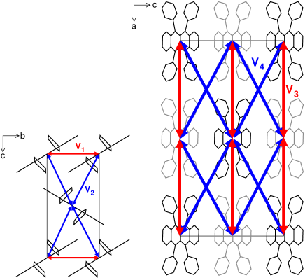
Figure 8: (Color online) The most important hopping paths in the rubrene crystal. Direction of view is parallel to the $a$ axis (left) and the $b$ axis (right) respectively. The black and the grey monomers have a different position in $b$ direction.

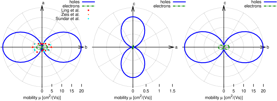
Figure 9: (Color online) The mobility for holes and electrons in the rubrene crystal in the $ba$ plane (left), $ac$ plane (middle) and $bc$ plane (right). The parameters are $F=10^{7}$ V/m, $T=300$ K. For comparison some experimental values for hole mobilities Ling et al. (2007); Zeis et al. (2006); Sundar et al. (2004) are plotted for the $ba$ plane.

In contrast to pentacene, the electronic coupling for holes and electrons in rubrene differs remarkably. That is why the calculated mobility for electrons is about one order of magnitude smaller than for holes, see Fig. 9. But unlike pentacene, the angular dependence of the mobility is qualitatively the same for both types of charge carriers. For holes a three dimensional depiction is shown in Fig. 10. The maximum mobility (20 cm²/V s for holes and 3 cm²/V s for electrons) is in $b$ direction because of the short lattice constant in that direction and the resulting strong electronic coupling. The lowest mobility (0.03 cm²/V s for holes and 0.003 cm²/V s for electrons) is in $a$ direction. The main contribution to the mobility in that direction are the zig-zag jumps between the planes perpendicular to $b$ which are marked with $V_{3}$ in Fig. 8 and the zig-zag jumps between the planes perpendicular to the $c$ axis marked with $V_{4}$. The corresponding couplings are more than one order of magnitude smaller than the next highest coupling $V_{2}$. The zig-zag jumps corresponding to $V_{2}$ are the main contribution to the mobility in $c$ direction.

Figure 10: (Color online) The mobility for holes in the rubrene crystal in all three dimensions. The parameters are the same as in Fig. 9.

Figure 9 shows some experimental mobility values for holes for the $ba$ plane. Sundar et al. (2004); Zeis et al. (2006); Ling et al. (2007) As for pentacene the calculation overestimates the mobility. The calculated maximum mobility is four times larger than the measured value. The mobilities for pentacene and rubrene calculated in Ref. Wen et al., 2009b with a similar approach seem to fit better to the experiment. Yet it seems that in their calculation a wrong dwell time of the charge carriers was used (cf. Sec. II.2).

The reorganization energy for rubrene is much higher than for pentacene. It was shown that the low-frequency bending of the phenyl side-groups in rubrene around the tetracene backbone contributes strongly to $\lambda$. da Silva Filho et al. (2005) However, this bending might be impeded in the crystal and a smaller reorganization energy would lead to an even higher mobility.

Temperature-dependent measurements in rubrene have shown a decrease of the mobility around room temperature. Podzorov et al. (2004); de Boer et al. (2004) This is an indication for band transport. However, the qualitative anisotropy of the mobility calculated with the hopping model fits quite well to the measurements.

III.2.3 PBI-F₂

The core-fluorinated perylene bisimide PBI-F₂ described by Schmidt et al. Schmidt et al. (2007) and depicted in Fig. 4c was analyzed. This material is quite interesting for application since it is remarkably air stable because of its electron-withdrawing substituents which makes the electrons less susceptible to trapping with oxygen. The planarity of the perylene core is only slightly distorted by the core fluorination which leads to a torsion angle of $3^{\circ}$. Schmidt et al. (2007) It was shown that PBI-F₂ has a narrower valence band and a broader conduction band than the unsubstituted PBI, mainly due to the altered molecular packing. Delgado et al. (2010) The unit cell contains two differently orientated monomers. In contrast to pentacene and rubrene, PBI-F₂ is an electron conductor which is caused by its high electron affinity. The electronic couplings for electrons and holes differ remarkably. The strongest couplings are collected in Tab. 4. The couplings which are not listed are at least one order of magnitude smaller than the smallest coupling mentioned. The strongest coupling for electron transport is found between monomers shifted along the $b$ direction, see Fig. 11. Note that this is about 300 times bigger than the coupling next in size, which is the one between two differently orientated monomers within the same unit cell. The result is an almost one dimensional charge transport along the $b$ direction, see Fig. 12 and 13. This might be problematic for application, since the charge transport gets very sensitive to lattice distortions, because the electron cannot easily pass at lattice defects which cannot be avoided in real crystals.

Table 4: The most important electronic couplings and the reorganization energy in the PBI-F₂ crystal for electrons and holes, cf. Fig. 11.

	$h^{+}$ [meV]	$e^{-}$ [meV]	$h^{+}$ [meV] Ref. Delgado et al.,2010	$e^{-}$ [meV] Ref. Delgado et al.,2010
$V_{1}$	0.251	129.234	2	107
$V_{2}$	2.398	0.452
$V_{3}$	0.010	0.017
$V_{4}$	0.003	0.004
$V_{5}$	0.001	0.002
$\lambda$	213	303	215 (213)	309 (307)

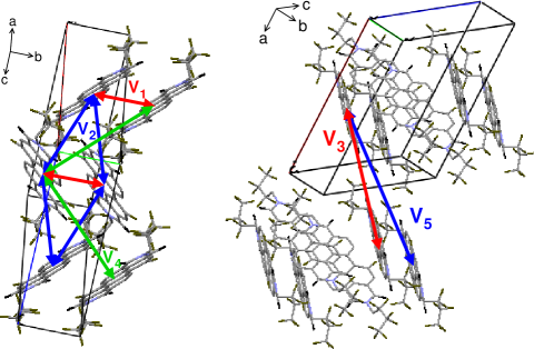
Figure 11: (Color online) The most important hopping paths in the PBI-F₂ crystal.

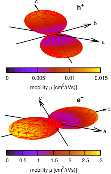
Figure 12: (Color online) The mobility for holes (top) and electrons (bottom) in the PBI-F₂ crystal in all three dimensions. The parameters are $F=10^{7}$ V/m, $T=300$ K.

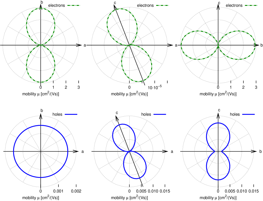
Figure 13: (Color online) The mobility for electrons and holes in the PBI-F₂ crystal in the $ab$ plane (left), $ac$ plane (middle) and $bc$ plane (right). The parameters are $F=10^{7}$ V/m, $T=300$ K.

Whereas the coupling between $b$ shifted monomers is very strong for electrons, this is surprisingly not the case for holes. Their coupling is more than two orders of magnitude smaller than the electron coupling. This is confirmed by other calculations. Delgado et al. (2010) The reason can be found in the differing nodal structure of the HOMO and the LUMO orbital for that dimer, see Fig. 14. By sliding one monomer relative to the other along the long axis, the coupling for holes oscillates depending on the displacement around zero, Delgado et al. (2010) because the overlap of the two HOMO orbitals with same and different phase alternate. All the other coupling constants do not differ significantly for the two types of charge carriers. This sole difference in the coupling results in a maximum electron mobility that is two orders of magnitude bigger than the maximum hole mobility, which is achieved in $c$ direction. However, in the plane perpendicular to $b$, the hole mobility is two orders of magnitude bigger than that of electrons, see Fig. 13.

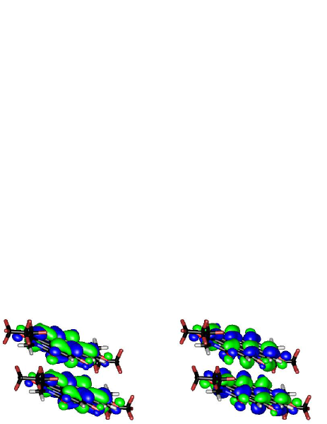
Figure 14: (Color online) The PBI-F₂ HOMO (left) and the LUMO (right) orbital for the dimer which is built by a $b$ shift and leads to the coupling $V_{1}$, compare Tab. 4 and Fig. 11.

The calculated reorganization energies, 303 meV for electrons and 213 meV for holes, is bigger than those for rubrene and pentacene. The values are in very good agreement with reorganization energies calculated by Delgado et al. Delgado et al. (2010) (309 and 307 meV for electrons, 215 and 213 meV for holes).

In order to test our master equation approach, some calculations were verified with Monte Carlo calculations. The results of both methods agree very well within the error bars of the Monte Carlo method. As an example Fig. 15 shows the mobility of PBI-F₂ in the $ab$ plane calculated with both approaches. The Monte Carlo simulations have run for at least 10 ns and have been averaged over at least 100 simulation runs, leading to a relative average error of less than 1 %. For this example the master equation approach required about 80.000 times less CPU time than the Monte Carlo approach. Thus the master equation approach is clearly advantageous as it is exact within the numerical accuracy of the computer while the Monte Carlo approach contains significant and slowly converging statistical errors.

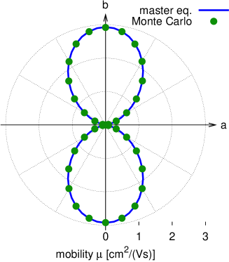
Figure 15: (Color online) Comparison of master equation and Monte Carlo results for the electron mobility in PBI-F₂ in the $ab$ plane. The parameters are $F=10^{7}$ V/m, $T=300$ K. The two methods show very good agreement.

III.2.4 PBI-(C₄F₉)₂

A further fluorinated perylene bisimide was investigated which was described by Li et al. Li et al. (2008) The four most important electronic couplings are listed in Tab. 5 and depicted in Fig. 16. In contrast to the other molecules it is striking that there is no symmetry-caused degeneration of the electronic couplings. It is furthermore important to notice that the intra-column couplings $V_{1}$ and $V_{2}$ along the $\pi$ stacks, which are parallel to the $a$ axis, differ by a factor of 3. This leads to a “trapping” of the charge carrier between the monomers which are coupled by $V_{1}$ as described in Sec. II.2: After jumping from one monomer to the next one along $V_{1}$, the charge carrier is more likely to jump back to the first monomer than to move on along $V_{2}$. To illustrate this trapping a charge trajectory along the $a$ axis, simulated by Monte Carlo, is drawn in Fig. 17 (top). One clearly sees that the charge carrier very often oscillates between two sites which lowers the mobility of the charge along the stacks. For comparison, a charge trajectory in PBI-F₂ along the high mobility axis is also depicted. No oscillatory motions can be found there.

Table 5: The most important electronic couplings and the reorganization energy in the PBI-(C₄F₉)₂ crystal for electrons, cf. Fig. 16.

	$e^{-}$ [meV]	$e^{-}$ [meV] Ref. Di Donato et al. (2010)
$V_{1}$	97.7	95.7
$V_{2}$	33.7	35.0
$V_{3}$	2.1	2.2
$V_{4}$	1.1	0.9
$\lambda$	339	360

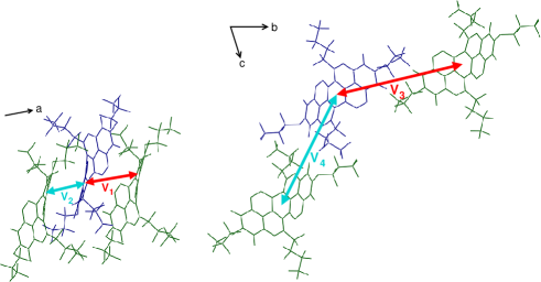
Figure 16: (Color online) The most important hopping paths in the PBI-(C₄F₉)₂ crystal.

Figure 17: Projection of the charge trajectory onto the respective direction with the highest mobility for PBI-(C₄F₉)₂ ($a$ direction, top) and PBI-F₂ ($b$ direction, bottom). The parameters are $F=10^{7}$ V/m, $T=300$ K.

This peculiarity of PBI-(C₄F₉)₂ becomes important when calculating the mobility: Because of the “trapping” that is caused by these oscillations, the mobility calculated with Eq. (15) or (16) and the Einstein relation (11) is severely overestimated, see Fig. 18. The green dotted curve is calculated without external field with the master equation along with Eq. (15) or (16) respectively, which is often used in literature. The red solid curve is also obtained by the master equation but the direct equation for the mobility, Eq. (10), was applied. The maximum mobility between these two curves differ by a factor of 2.4. Besides that, the calculation using the diffusion coefficient and the Einstein relation even results in a wrong angle for the maximum mobility. To prove that the result of Eq. (10) (red solid line) is the right one, Monte Carlo simulations were conducted (blue points). The simulations ran for 10 ns and $\langle x\rangle$ and $\langle(x-\langle x\rangle)^{2}\rangle$ were averaged over 1000 trajectories. The relative average error was about 0.4 % and the deviation of the master equation from Monte Carlo was about 0.2 %. The differences in the results of Eq. (15) or (16) and (10) are not caused by the electric field. This is shown by the black dashed line which was calculated with Eq. (15) but with the same field as for the red solid line. One clearly sees that the black dashed line does not coincide with the red line but with the green line (calculated without field) instead, proving that this approach cannot be applied.

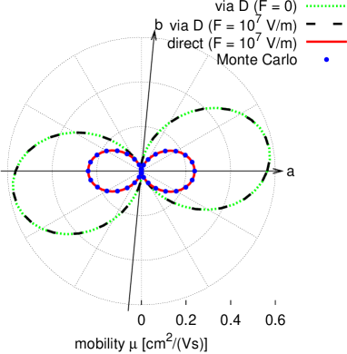
Figure 18: (Color online) Comparison of the mobility in the $ab$ plane of PBI-(C₄F₉)₂ calculated via the diffusion coefficient (Eq. (15)) and the Einstein relation (Eq. (11)) for $F=0$ (green, dotted) and $F=10^{7}$ V/m (black, dashed), calculated directly (Eq. (10), red, solid) and calculated with Monte Carlo (Eq. (17), blue points) for $F=10^{7}$ V/m ($T=300$ K in all cases).

IV Summary and conclusions

A quantum chemical protocol for calculating the charge carrier mobilities in organic semiconductor crystals was presented. A hopping model using Marcus theory has been implemented by means of the master equation approach which is more than four orders of magnitude faster than the Monte Carlo method and free from statistical errors. In contrast to the master equation, the Monte Carlo approach allows to simulate the transport parameters with a time dependent framework. However, since this is a stochastic method many simulation runs are needed in order to achieve an acceptable statistical error. Furthermore, it is important to make sure that the stationary state is obtained within the simulation time. This is a serious problem for disordered materials. Solving the matrix equation (4) describing the stationary state instead by means of analytic numerical methods guarantees the stationary solution.

The mobility is often calculated without external field and without the master equation by calculating the diffusion coefficient and applying the Einstein relation. However it can easily happen that the diffusion coefficient is overestimated in amorphous materials and even in perfect crystals due to to a “trapping” of the charge between energetically similar sites. That is why it is more appropriate to calculate the mobility by means of the master equation from the charge drift velocity. The obtained results fit perfectly with those of Monte Carlo simulations. It is advisable even to calculate the diffusion coefficient out of the mobility by applying the Einstein relation, because in the Eq. (10) for the mobility, the trapping cancels. It was shown that the Einstein relation even holds for extremely energetically disordered materials for not too high electric fields.

The angular dependence of the mobility in pentacene, rubrene, PBI-F₂ and PBI-C₄F₉ was calculated and the results were correlated with the morphology of the crystals. The results for pentacene and rubrene show a good qualitative agreement with experimental data. However, the absolute values of the mobilities are strongly overestimated as he assumption of localized charge carriers that move in a hopping process without any interaction with nonlocal lattice vibrations is not completely adequate for organic crystals. Nevertheless this simple model allows for qualitative transport property predictions. It was shown that PBI-F₂ appears to be an almost one dimensional n-type semiconductor.

Appendix A

Equation (15) is valid even if an external field is applied because in this approach the resulting drift is not caused by different jump distances parallel or antiparallel to the field respectively since these distances $\vec{r}_{ji}$ are fixed by the monomer positions. Instead the field influences the jump rates $\nu_{ji}$, cf. Eq. (1). The drift contribution to the jump rate would have to be added to or subtracted from the actual rate respectively. However, since $\nu_{ji}$ influences the diffusion linearly, the drift cancels when summing across all lattice sites. In order to verify this we have computed the solution of the time dependent master equation

$$\frac{d}{dt}\vec{p}=\mathbf{N}\vec{p},$$ (26)

which reads

$$\vec{p}(t)=\sum_{i}\vec{c}_{i}\mathrm{e}^{l_{i}t},$$ (27)

with the eigenvalues $l_{i}$ and the respective eigenvectors $\vec{c}_{i}$. The diffusion constant can now be calculated via

$$D = \frac{1}{2}\frac{d}{dt}\langle(x(t)-\langle x\rangle(t))^{2}\rangle$$ (28)

$$= \frac{1}{2}\frac{d}{dt}\sum_{i}\left(p_{i}(t)x_{i}-\sum_{j}p_{j}(t)x_{j}\right)^{2},$$

where the summation is across all sites which positions are $x_{i}$. We have used the Gaussian disorder model described in Sec. II.5 using the Miller-Abrahams hopping rate, Eq. (25), for the entries of the matrix $\mathbf{N}$, cf. Eq. (5). Additionally we have used a simple biased random walk where the mobility and the diffusion can even be calculated analytically. Our calculations confirmed that Eq. (15) leads to exactly the same results as Eq. (28) as long as there is no energetic disorder, i.e. $\varrho(E)=\delta(E)$, cf. Eq. (21). The reason for the deviations in the case $\sigma\neq 0$ have already been explained in detail in Sec. II.2.

References

- Armstrong et al. (2009) N. R. Armstrong, W. Wang, D. M. Alloway, D. Placencia, E. Ratcliff, and M. Brumbach, Macromol. Rapid Commun. 30, 717 (2009).
- Meerheim et al. (2009) R. Meerheim, B. Luessem, and K. Leo, Proc. of the IEEE 97, 1606 (2009).
- Kulkarni et al. (2004) A. P. Kulkarni, C. J. Tonzola, A. Babel, and S. A. Jenekhe, Chem. Mater. 16, 4556 (2004).
- Dimitrakopoulos and Malenfant (2002) C. Dimitrakopoulos and P. Malenfant, Adv. Mater. 14, 99 (2002).
- Newman et al. (2004) C. R. Newman, C. D. Frisbie, D. A. da Silva Filho, J.-L. Brédas, P. C. Ewbank, and K. R. Mann, Chem. Mater. 16, 4436 (2004).
- Facchetti (2007) A. Facchetti, Mater. Today 10, 28 (2007).
- Subramanian et al. (2005) V. Subramanian, P. Chang, J. Lee, S. Molesa, and S. Volkman, IEEE Transactions on Components and Packaging Technologies 28, 742 (2005).
- Myny et al. (2010) K. Myny, S. Steudel, S. Smout, P. Vicca, F. Furthner, B. van der Putten, A. Tripathi, G. Gelinck, J. Genoe, W. Dehaene, and P. Heremans, Organic Electronics 11, 1176 (2010).
- Riede et al. (2008) M. Riede, T. Mueller, W. Tress, R. Schueppel, and K. Leo, Nanotechnology 19, 424001 (2008).
- Kippelen and Brédas (2009) B. Kippelen and J.-L. Brédas, Energy Environ. Sci. 2, 251 (2009).
- Dennler et al. (2009) G. Dennler, M. C. Scharber, and C. J. Brabec, Adv. Mater. 21, 1323 (2009).
- Chidichimo and Filippelli (2010) G. Chidichimo and L. Filippelli, International Journal of Photoenergy 2010, Article ID 123534 (2010).
- Deibel and Dyakonov (2010) C. Deibel and V. Dyakonov, Rep. Prog. Phys. 73, 096401 (2010).
- Brédas et al. (2009) J.-L. Brédas, J. E. Norton, J. Cornil, and V. Coropceanu, Accounts of Chemical Research 42, 1691 (2009).
- Holstein (1959) T. Holstein, Ann. Phys. 8, 343 (1959).
- Peierls (1955) R. E. Peierls, Quantum theory of solids, 1st ed. (Oxford University Press, 1955).
- Hannewald et al. (2004) K. Hannewald, V. M. Stojanović, J. M. T. Schellekens, P. A. Bobbert, G. Kresse, and J. Hafner, Phys. Rev. B 69, 075211 (2004).
- Hannewald and Bobbert (2004) K. Hannewald and P. A. Bobbert, Appl. Phys. Lett. 85, 1535 (2004).
- Ortmann et al. (2010a) F. Ortmann, F. Bechstedt, and K. Hannewald, New J. Phys. 12, 023011 (2010a).
- Ortmann et al. (2010b) F. Ortmann, F. Bechstedt, and K. Hannewald, J. Phys.: Condens. Matter 22, 465802 (2010b).
- Troisi et al. (2005) A. Troisi, G. Orlandi, and J. E. Anthony, Chem. Mater. 17, 5024 (2005).
- Troisi and Orlandi (2006) A. Troisi and G. Orlandi, Phys. Rev. Lett. 96, 086601 (2006).
- Troisi (2007) A. Troisi, Adv. Mater. 19, 2000 (2007).
- Stafström (2010) S. Stafström, Chem. Soc. Rev. 39, 2484 (2010).
- Schein et al. (1978) L. B. Schein, C. B. Duke, and A. R. McGhie, Phys. Rev. Lett. 40, 197 (1978).
- Brédas et al. (2002) J. L. Brédas, J. P. Calbert, D. A. da Silva Filho, and J. Cornil, Proc. Natl. Acad. Sci. U.S.A. 99, 5804 (2002).
- Herbst and Hunger (1997) W. Herbst and K. Hunger, Industrial Organic Pigments: Production, Properties, Applications, 2nd ed. (Wiley-VCH, 1997).
- Langhals et al. (1998) H. Langhals, J. Karolin, and L. B-A. Johansson, J. Chem. Soc., Faraday Trans. 94, 2919 (1998).
- Struijk et al. (2000) C. W. Struijk, A. B. Sieval, J. E. J. Dakhorst, M. van Dijk, P. Kimkes, R. B. M. Koehorst, H. Donker, T. J. Schaafsma, S. J. Picken, A. M. van de Craats, J. M. Warman, H. Zuilhof, and E. J. R. Sudhölter, J. Am. Chem. Soc. 122, 11057 (2000).
- Chen et al. (2004) Z. Chen, M. G. Debije, T. Debaerdemaeker, P. Osswald, and F. Würthner, ChemPhysChem 5, 137 (2004).
- An et al. (2005) Z. An, J. Yu, S. C. Jones, S. Barlow, S. Yoo, B. Domercq, P. Prins, L. D. A. Siebbeles, B. Kippelen, and S. R. Marder, Adv. Mater. 17, 2580 (2005).
- Schmidt et al. (2007) R. Schmidt, M. M. Ling, J. H. Oh, M. Winkler, M. Könemann, Z. B. 2, and F. Würthner, Adv. Mater. 19, 3692 (2007).
- Chen et al. (2007) H. Z. Chen, M. M. Ling, X. Mo, M. M. Shi, M. Wang, and Z. Bao, Chem. Mater. 19, 816 (2007).
- Weitz et al. (2008) R. T. Weitz, K. Amsharov, U. Zschieschang, E. B. Villas, D. K. Goswami, M. Burghard, H. Dosch, M. Jansen, K. Kern, and H. Klauk, J. Am. Chem. Soc. 130, 4637 (2008).
- Molinari et al. (2009) A. S. Molinari, H. Alves, Z. Chen, A. Facchetti, and A. F. Morpurgo, J. Am. Chem. Soc. 131, 2462 (2009).
- Wen et al. (2009a) Y. Wen, Y. Liu, C. an Di1, Y. Wang, X. Sun, Y. Guo, J. Zheng, W. Wu, S. Ye, and G. Yu, Adv. Mater. 21, 1631 (2009a).
- Zhan et al. (2007) X. Zhan, Z. Tan, B. Domercq, Z. An, X. Zhang, S. Barlow, Y. Li, D. Zhu, B. Kippelen, and S. R. Marder, J. Am. Chem. Soc. 129, 7246 (2007).
- Wöhrle et al. (1995) D. Wöhrle, L. Kreienhoop, G. Schnurpfeil, J. Elbe, B. Tennigkeit, S. Hiller, and D. Schlettwein, J. Mater. Chem. 5, 1819 (1995).
- Schmidt-Mende et al. (2001) L. Schmidt-Mende, A. Fechtenkötter, K. Müllen, E. Moons, R. H. Friend, and J. D. MacKenzie, Science 293, 1119 (2001).
- Shin et al. (2006) W. S. Shin, H.-H. Jeong, M.-K. Kim, S.-H. Jin, M.-R. Kim, J.-K. Lee, J. W. Lee, and Y.-S. Gal, J. Mater. Chem. 16, 384 (2006).
- Wen et al. (2009b) S.-H. Wen, A. Li, J. Song, W.-Q. Deng, K.-L. Han, and W. A. Goddard III, J. Phys. Chem. B 113, 8813 (2009b).
- Liu et al. (2010) Y.-H. Liu, Y. Xie, and Z.-Y. Lu, Chem. Phys. 367, 160 (2010).
- Deng and Goddard III (2004) W.-Q. Deng and W. A. Goddard III, J. Phys. Chem. B 108, 8614 (2004).
- Coropceanu et al. (2007) V. Coropceanu, J. Cornil, D. A. da Silva Filho, Y. Olivier, R. Silbey, and J.-L. Brédas, Chem. Rev. 107, 926 (2007).
- Harada et al. (2005) K. Harada, A. G. Werner, M. Pfeiffer, C. J. Bloom, C. M. Elliott, and K. Leo, Phys. Rev. Lett. 94, 036601 (2005).
- Pautmeier et al. (1991) L. Pautmeier, R. Richert, and H. Bässler, Philos. Mag. B 63, 587 (1991).
- Borsenberger et al. (1991) P. M. Borsenberger, L. Pautmeier, R. Richert, and H. Bässler, J. Chem. Phys. 94, 8276 (1991).
- Casado and Mejias (1994) J. M. Casado and J. J. Mejias, Philos. Mag. B 70, 1111 (1994).
- Baranovskii et al. (1998a) S. D. Baranovskii, T. Faber, F. Hensel, and P. Thomas, J. Non-Cryst. Solids 227-230, 158 (1998a).
- Mattheus et al. (2001) C. C. Mattheus, A. B. Dros, J. Baas, A. Meetsma, J. L. de Boer, and T. T. M. Palstra, Acta Cryst. C 57, 939 (2001).
- Malagoli et al. (2004) M. Malagoli, V. Coropceanu, D. A. da Silva Filho, and J. L. Brédas, J. Chem. Phys. 120, 7490 (2004).
- Jurchescu et al. (2004) O. D. Jurchescu, J. Baas, , and T. T. M. Palstra, Appl. Phys. Lett. 84, 3061 (2004).
- Lee et al. (2006) J. Y. Lee, S. Roth, and Y. W. Park, Appl. Phys. Lett. 88, 252106 (2006).
- Sundar et al. (2004) V. C. Sundar, J. Zaumseil, V. Podzorov, E. Menard, R. L. Willett, T. Someya, M. E. Gershenson, and J. A. Rogers, Science 303, 1644 (2004).
- Podzorov et al. (2004) V. Podzorov, E. Menard, A. Borissov, V. Kiryukhin, J. A. Rogers, and M. E. Gershenson, Phys. Rev. Lett. 93, 086602 (2004).
- de Boer et al. (2004) R. W. I. de Boer, M. E. Gershenson, A. F. Morpurgo, and V. Podzorov, phys. stat. sol. (a) 201, 1302–1331 (2004).
- da Silva Filho et al. (2005) D. A. da Silva Filho, E.-G. Kim, and J.-L. Brédas, Adv. Mater. 17, 1072 (2005).
- Jurchescu et al. (2006) O. D. Jurchescu, A. Meetsma, and T. T. M. Palstra, Acta Cryst. B 62, 330 (2006).
- Zeis et al. (2006) R. Zeis, C. Besnard, T. Siegrist, C. Schlockermann, X. Chi, and C. Kloc, Chem. Mater. 18, 244 (2006).
- Ling et al. (2007) M.-M. Ling, C. Reese, A. L. Briseno, and Z. Bao, Synth. Met. 157, 257 (2007).
- Marcus (1956) R. A. Marcus, J. Chem. Phys. 129, 966 (1956).
- Marcus (1993) R. A. Marcus, Rev. Mod. Phys. 65, 599 (1993).
- Norton and Brédas (2008) J. E. Norton and J.-L. Brédas, J. Am. Chem. Soc. 130, 12377 (2008).
- McMahon and Troisi (2010) D. P. McMahon and A. Troisi, J. Phys. Chem. Lett. 1, 941 (2010).
- Picon et al. (2007) J.-D. Picon, M. N. Bussac, and L. Zuppiroli, Phys. Rev. B 75, 235106 (2007).
- Cheung and Troisi (2008) D. L. Cheung and A. Troisi, Phys. Chem. Chem. Phys. 10, 5941 (2008).
- Li et al. (2007) H. Li, J.-L. Brédas, and C. Lennartz, J. Chem. Phys. 126, 164704 (2007).
- Sancho-García and Pérez-Jiménez (2008) J. C. Sancho-García and A. J. Pérez-Jiménez, J. Chem. Phys. 129, 024103 (2008).
- Sancho-García et al. (2010) J. C. Sancho-García, A. J. Pérez-Jiménez, Y. Olivier, and J. Cornil, Phys. Chem. Chem. Phys. 12, 9381 (2010).
- Sancho-García and Pérez-Jiménez (2009) J. C. Sancho-García and A. J. Pérez-Jiménez, Phys. Chem. Chem. Phys. 11, 2741 (2009).
- Houili et al. (2006) H. Houili, E. T. s, I. Batistić, and L. Zuppiroli, J. Appl. Phys. 100, 033702 (2006).
- Yu et al. (2001) Z. G. Yu, D. L. Smith, A. Saxena, R. L. Martin, and A. R. Bishop, Phys. Rev. B 63, 085202 (2001).
- Landsberg (1981) P. T. Landsberg, Eur. J. Phys. 2, 213 (1981).
- Bisquert (2008) J. Bisquert, Phys. Chem. Chem. Phys. 10, 3175 (2008).
- Zhdanov (1985) V. Zhdanov, Surface Sci. 149, L13 (1985).
- Myshlyavtsev et al. (1995) A. V. Myshlyavtsev, A. A. Stepanov, C. Uebing, and V. P. Zhdanov, Phys. Rev. B 52, 5977 (1995).
- Gonzalez-Vazquez et al. (2009) J. P. Gonzalez-Vazquez, J. A. Anta, and J. Bisquert, Phys. Chem. Chem. Phys. 11, 10359 (2009).
- tur (2009) “TURBOMOLE V6.0, a development of University of Karlsruhe and Forschungszentrum Karlsruhe GmbH, 1989-2007, TURBOMOLE GmbH, since 2007; available from http://www.turbomole.com,” (2009).
- Dirac (1929) P. A. M. Dirac, Proc. R. Soc. Lond. A 123, 714 (1929).
- Slater (1951) J. C. Slater, Phys. Rev. 81, 385 (1951).
- Vosko et al. (1980) S. H. Vosko, L. Wilk, and M. Nusair, Can. J. Phys. 58, 1200 (1980).
- Becke (1988) A. D. Becke, Phys. Rev. A 38, 3098 (1988).
- Lee et al. (1988) C. Lee, W. Yang, and R. G. Parr, Phys. Rev. B 37, 785 (1988).
- Becke (1993) A. D. Becke, J. Chem. Phys. 98, 5648 (1993).
- Dunning (1989) T. H. Dunning, J. Chem. Phys. 90, 1007 (1989).
- Sánchez-Carrera et al. (2006) R. S. Sánchez-Carrera, V. Coropceanu, D. A. da Silva Filho, R. Friedlein, W. Osikowicz, R. Murdey, C. Suess, W. R. Salaneck, and J.-L. Brédas, J. Phys. Chem. B 110, 18904 (2006).
- Coropceanu et al. (2002) V. Coropceanu, M. Malagoli, D. A. da Silva Filho, N. E. Gruhn, T. G. Bill, and J. L. Brédas, Phys. Rev. Lett. 89, 275503 (2002).
- Anta et al. (2008) J. A. Anta, I. Mora-Sero, T. Dittrich, and J. Bisquert, Phys. Chem. Chem. Phys. 10, 4478 (2008).
- Novikov and Malliaras (2006) S. V. Novikov and G. G. Malliaras, phys. stat. sol. (b) 243, 291 (2006).
- Roichman and Tessler (2002) Y. Roichman and N. Tessler, Appl. Phys. Lett. 80, 1948 (2002).
- Baranovskii et al. (1998b) S. D. Baranovskii, T. Faber, F. Hensel, and P. Thomas, phys. stat. sol. (b) 205, 87 (1998b).
- Abkowitz et al. (1991) M. Abkowitz, H.Bässler, and M. Stolka, Philos. Mag. B 63, 201 (1991).
- Bässler (1993) H. Bässler, phys. stat. sol. (b) 175 (1993).
- Richert et al. (1989) R. Richert, L. Pautmeier, and H. Bässler, Phys. Rev. Lett. 63, 547 (1989).
- Miller and Abrahams (1960) A. Miller and E. Abrahams, Phys. Rev. 120, 745 (1960).
- Li et al. (2008) Y. Li, L. Tan, Z. Wang, H. Qian, Y. Shi, and W. Hu, Org. Lett. 10, 529 (2008).
- Delgado et al. (2010) M. C. R. Delgado, E.-G. Kim, D. A. da Silva Filho, and J.-L. Brédas, J. Am. Chem. Soc. 132, 3375 (2010).
- Di Donato et al. (2010) E. Di Donato, R. P. Fornari, S. Di Motta, Y. Li, Z. Wang, and F. Negri, J. Phys. Chem. B 114, 5327 (2010).