SHREC 2011: robust feature detection and description benchmark
Abstract
Feature-based approaches have recently become very popular in computer vision and image analysis applications, and are becoming a promising direction in shape retrieval. SHREC’11 robust feature detection and description benchmark simulates the feature detection and description stages of feature-based shape retrieval algorithms. The benchmark tests the performance of shape feature detectors and descriptors under a wide variety of transformations. The benchmark allows evaluating how algorithms cope with certain classes of transformations and strength of the transformations that can be dealt with. The present paper is a report of the SHREC’11 robust feature detection and description benchmark results.
Information storage and retrievalH.3.2Information Search and RetrievalRetrieval models \CCScatArtificial intelligenceI.2.10Vision and Scene UnderstandingShape
:
\CCScat1 Introduction
Feature-based approaches have recently become very popular in computer vision and image analysis applications, notably due to the works of Lowe [Low04], Sivic and Zisserman [SZ03], and Mikolajczyk and Schmid [MS05]. In these approaches, an image is described as a collection of local features (“visual words”) from a given vocabulary, resulting in a representation referred to as a bag of features. The bag of features paradigm relies heavily on the choice of the local feature descriptor that is used to create the visual words. A common evaluation strategy of image feature detection and description algorithms is the stability of the detected features and their invariance to different transformations applied to an image. In shape analysis, feature-based approaches have been introduced more recently and are gaining popularity in shape retrieval applications.
SHREC’11 invariant feature detection and description benchmark simulates the feature detection and description stages of feature-based shape retrieval algorithms. The benchmark tests the performance of shape feature detectors and descriptors under a wide variety of different transformations. The benchmark allows evaluating how algorithms cope with certain classes of transformations and what is the strength of the transformations that can be dealt with.
This report presents a long version of the paper [BBB∗11].
2 Data
The dataset used in this benchmark was from the TOSCA shapes [BBK08], available in the public domain. The shapes were represented as triangular meshes with approximately 10,000–50,000 vertices.
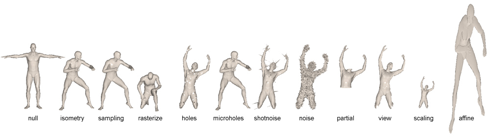
The dataset includes ones shape class (human) with simulated transformations. Compared to the SHREC 2010 benchmark, there are additional transformation classes and the transformations themselves are more challenging. For each null shape, transformations were split into 11 classes shown in Figure 1: isometry (non-rigid triangulation- and distance-preserving almost inelastic deformations), topology (welding of shape vertices resulting in different triangulation), rasterization (simulating non-pointwise topological artifacts due to occlusions in 3D geometry acquisition), view (simulating missing parts due to 3D acquisition artifacts), partial (missing parts), micro holes and big holes, global uniform scaling, global affine transformations, additive Gaussian noise, shot noise, down-sampling (less than 20% of the original points).
In each class, the transformation appeared in five different versions numbered 1–5. In all shape categories except scale and isometry, the version number corresponded to the transformation strength levels: the higher the number, the stronger the transformation (e.g., in noise transformation, the noise variance was proportional to the strength number). For the isometry class, the numbers do not reflect the strength of the transformation. The total number of transformations was 55. The dataset is available at http://tosca.cs.technion.ac.il/book/shrec_feat.html.
3 Evaluation methodology
The evaluation was performed separately for feature detection and feature description algorithms. Feature detectors were further divided into point and region; feature descriptors were divided into point, region, and dense. The participants were asked to provide, for each shape in the dataset, (i) a set of detected feature points or regions ; (ii) optionally, for each detected point , a descriptor vector ; or alternatively, for each detected region , a descriptor vector . For dense descriptors, participants provided . The performance was measured by comparing features and feature descriptors computed for transformed shapes and the corresponding null shapes.
3.1 Feature detection
The quality of the feature detection was measured using the repeatability criterion. Assuming for each transformed shape in the dataset the groundtruth dense correspondence to the null shape to be given in the form of pairs of points , a feature point is said to be repeatable if a geodesic ball of radius around the corresponding point contains a detected feature point .111Features without groundtruth correspondence (e.g. in regions in the null shape corresponding to holes in the transformed shape) are ignored. Repeatable features are
where and denotes the geodesic distance function in .
Similarly, for region detectors, a region is repeatable if the corresponding region has overlap larger than ,
The repeatability of a feature detector is defined as the percentage of features that are repeatable, the definition being dependent of whether a point or region descriptor is used.
3.2 Feature description
Let , denote descriptors computed on feature points and , respectively. For point descriptors, we consider as the point corresponding to the closest point to , where , such that for some .
Descriptor quality was evaluated using the normalized distance between descriptors at corresponding points,
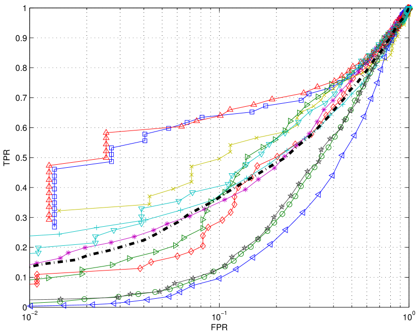
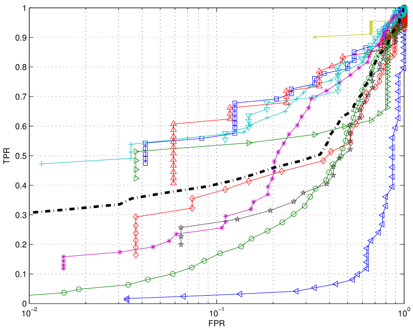
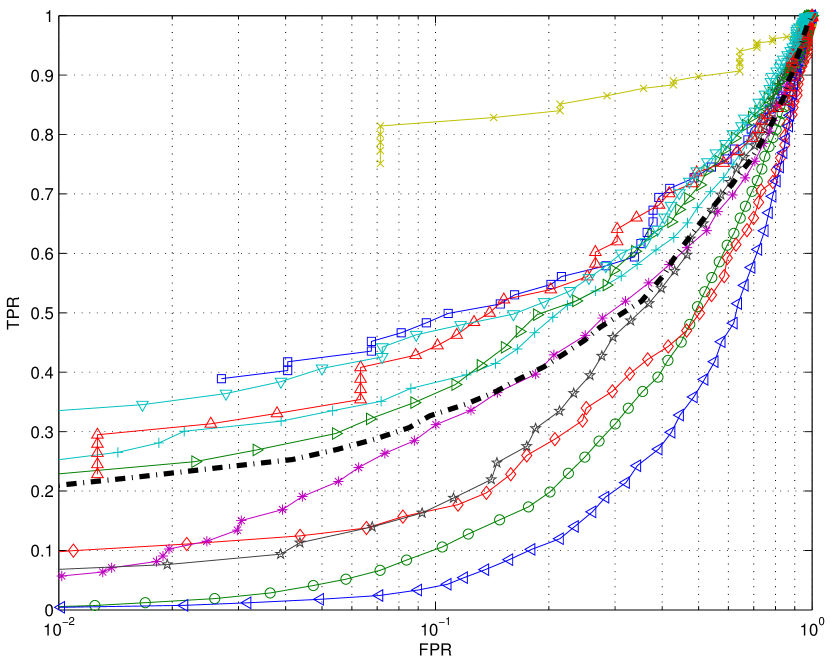
In addition, an evaluation using the ROC was performed as follows. The corresponding feature points are considered true positives if , for some threshold . The true positive rate is defined as ; the false positive rate is defined as . By varying the threshold , a set of pairs referred to as the receiver operation characteristic (ROC) curve is obtained. For a fixed FPR, the higher the TPR, the better.
For a dense descriptor, the quality is measured as the average normalized distance between the descriptor vectors in corresponding points,
4 Feature detection methods
4.1 Point features
Harris 3D (Sipiran and Bustos [SB10]). The algorithm proposes an extension for meshes of the Harris corner detection method [HS88]. The algorithm suggests to determine a neighborhood (rings or adaptive) around a vertex. Next, this neighborhood is used to fit a quadratic patch which is considered as an image. After applying a gaussian smoothing, derivatives are calculated which are used to calculate the Harris response for each vertex. In this benchmark, three different configurations were used: adaptive neighborhoods with , 1-ring neighborhoods , and 2-ring neighborhoods. For details, see [SB10].
Mesh-DoG (Zaharescu et al. [ZBVH09] ). The method considers the general setting of 2-D manifolds embedded in endowed in with a scalar function , such as colour or curvature. This represents a generalization of 2-D images, that can be viewed as a uniformly sampled square grid with vertices of valence 4. Operators, such as the gradient and the convolution are defined in this context. A scale-space representation of the scalar function is build using iterative convolutions with a Guassian kernel. Feature detection consists of two steps. Firstly, the extrema of the function’s Laplacian (approximated by taking the difference between adjacent scales - Difference of Gaussian) are found across scales, followed by non-maximum suppression using a 1-ring neighbourhood both spatially and across adjacent scales. Secondly, the detected extrema are thresholded (400 points). Mean and Gaussian curvature computed using [MDSB02] were the scalar functions used for current tests. For exact details and settings, see [ZBVH09].
Mesh SIFT (Smeets et al. [MFK∗10]). The Mesh SIFT detector detects scale space extrema as local feature locations. First, a scale space is constructed containing smoothed versions of the input mesh, which are obtained by subsequent convolutions of the mesh with a binomial filter. Next, for the detection of salient points in the scale space, the mean curvature (Mesh SIFT-H) and the principal coordinates in curvature space (Mesh SIFT-KK), which are minimal and maximal curvature, are computed for each vertex and at each scale in the scale space ( and ). Note that the mesh is smoothed and not the function on the mesh ( or ). Scale space extrema in scale spaces of differences between subsequent scales ( for Mesh SIFT-H and for Mesh SIFT-KK) are finally selected as local feature locations.
Mesh-Scale DoG (Darom and Keller [DK11]) We follow the work of Zaharescu et al. [ZBVH09] that presented a Difference of Gaussians based feature points detector for mesh objects. We propose to define a Gaussian filter on the mesh geometry, and compute a set of filtered meshes. Consecutive octaves are subtracted to compute the DoG function, and define the local maxima (both in location and scale) as our feature points at that point and scale. In order to make the detected features scale invariant, we suggest to set the support for each feature point to the width of the filter at that scale. For details, see [DK11].
4.2 Region detectors
Shape MSER (Litman et al. [LBB10]). The algorithm finds maximally stable components in 3D shapes, similarly to the popular MSER method for feature analysis in images [MCUP04]. The shape is represented as a component tree based on vertex- or edge-wise weighting function (VW and EW, respectively). In this benchmark, three different weights were used: edge weighting by inverse of commute time kernel (EW 1/CT) and inverse heat kernel (EW 1/HKS), and vertex weighting by heat kernel diagonal (VW HKS). For details, see [LBB10].
5 Feature description methods
5.1 Point descriptors
Mesh-HoG (Zaharescu et al. [ZBVH09] ). For a given interest point, the descriptor is computed using a geodesic support region, proportional to of the total surface area. For each vertex in the neighbourhood, the 3-D gradient information is computed using at the detected scale. As a first step, a local coordinate system is chosen, in order to make the descriptor rotation invariant. Then, a histogram of gradient is computed, both spatially, at a coarse level, in order to maintain a certain high-level spatial ordering, and using orientations, at a finer level. Since the gradient vectors are 3 dimensional, the histograms are computed in 3D. The histograms are concatenated and normalized. A dimensional descriptor is obtained. The gradient of the participating neighbouring vertices is computed at the scale of the detected interest point. For exact details and settings, see [ZBVH09].
Scale Invariant Spin Image (Darom and Keller [DK11]) The Spin Image local descriptor was presented by Johnson and Hebert [JH99], and has gained popularity due to its robustness and simplicity. Utilizing the local scale estimated by the Mesh-Scale DoG detector, we propose to derive a Scale Invariant Spin Image mesh descriptor, where we compute the Spin Image descriptor over the local scale estimated at the interest point. This improves feature point matching, in particular when the meshes are related significant partial matching. For details, see [DK11].
Local Depth SIFT (Darom and Keller [DK11]) The SIFT algorithm, presented by D. Lowe [Low04] is a state-of-the-art approach to computing scale and rotation invariant local features in images. The SIFT descriptor is based on computing a local radial-angular histogram of the pixel value derivatives. Inspired by Lowe’s seminal work, we propose to compute a new local feature for 3D meshes we denote Local Depth SIFT (LD-SIFT). Given an interest point we estimate its tangent plane, and compute the distance from each point on the surface to that plane to create a depth map, and set the viewport size to match the feature scale, as detected by the Mesh-Scale DoG detector. This makes our construction scale invariant. We compute the PCA of the the points surrounding the interest point, and use their dominant direction as the local dominant angle, and rotate the depth map to a canonical angle based on the dominant angle. This makes the LD-SIFT rotation invariant. We compute a SIFT feature descriptor on the resulting depth map to create the Local Depth SIFT feature descriptor. For details, see [DK11].
5.2 Dense descriptors
Generalized HKS (Zobel et al. [ZRHar]). The Generalized HKS is a generalization of the HKS [SOG09] to 1-forms (where a 1-form can be regarded as vector field). It is derived from the heat kernel for 1-forms in a similar way as the HKS is derived from the heat kernel for functions. This yields a symmetric tensor field of second order with a time parameter . For easier comparability we consider scalar tensor invariants. For details see [ZRHar] or [Zob10].
6 Results
6.1 Point feature detectors.
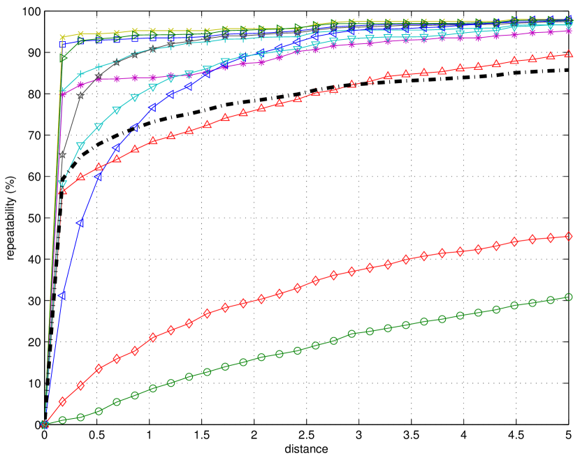
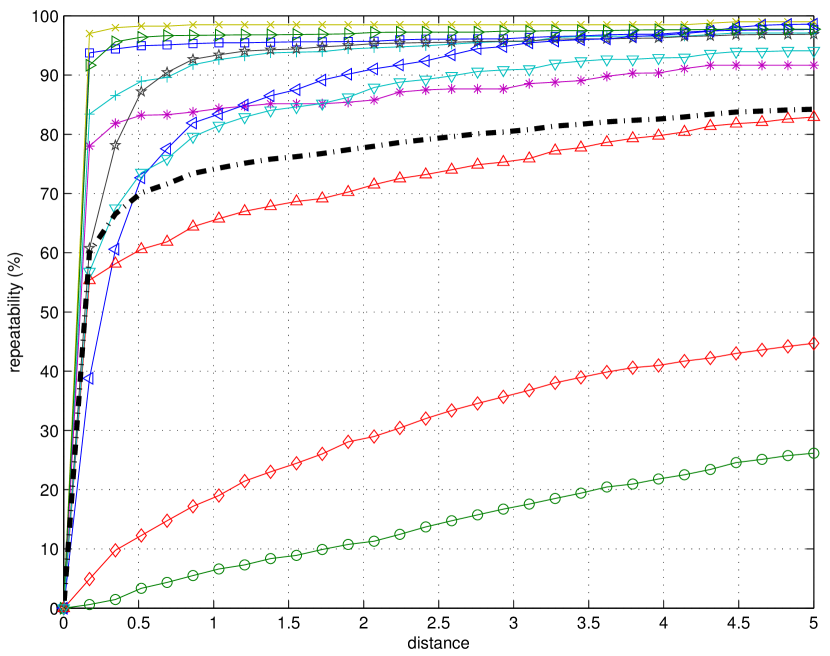
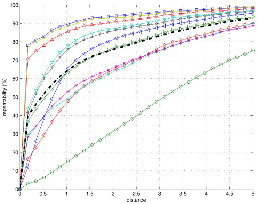
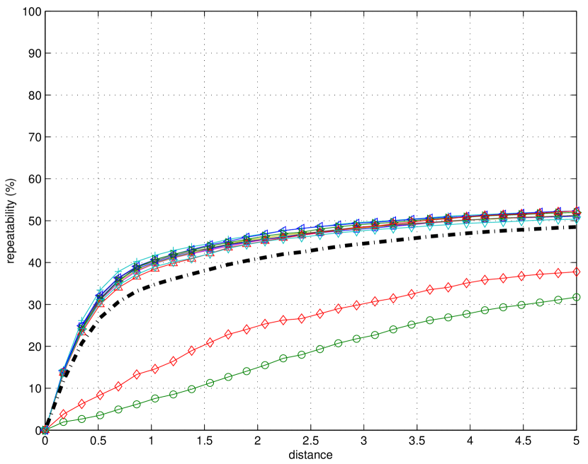
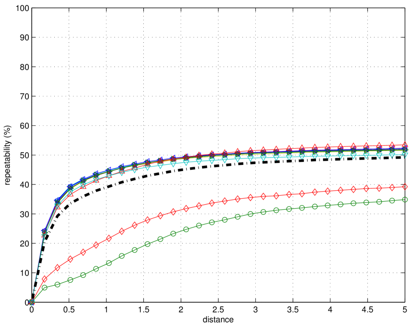
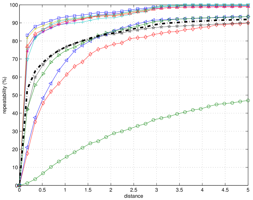
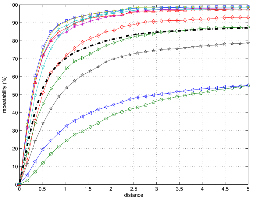
Tables 1–9 show the repeatability of different point descriptors at fixed radius (approximately of the shape diameter), broken down according to transformation classes and strengths. Higher repeatability scores are indication of better performance. Figures 2–3 show the repeatability of point descriptors as function of geodesic distance varying from to .
| Strength | |||||
|---|---|---|---|---|---|
| Transform. | 1 | 2 | 3 | 4 | 5 |
| Isometry | 97.75 | 98.13 | 97.92 | 97.94 | 97.70 |
| Rasterization | 35.50 | 37.75 | 36.17 | 34.19 | 30.85 |
| Sampling | 73.50 | 59.50 | 50.67 | 44.72 | 42.06 |
| Holes | 96.50 | 96.88 | 96.83 | 96.88 | 96.65 |
| Micro holes | 96.50 | 95.75 | 95.50 | 95.38 | 95.20 |
| Scaling | 98.00 | 98.00 | 98.00 | 98.00 | 98.00 |
| Affine | 98.25 | 98.75 | 98.50 | 98.13 | 97.45 |
| Noise | 99.25 | 99.13 | 98.50 | 98.25 | 97.95 |
| Shot Noise | 98.25 | 98.00 | 98.00 | 97.87 | 97.75 |
| Partial | 98.25 | 97.25 | 97.17 | 90.06 | 89.50 |
| View | 95.50 | 96.38 | 96.33 | 97.00 | 96.70 |
| Average | 89.75 | 88.68 | 87.60 | 86.22 | 85.44 |
| Strength | |||||
|---|---|---|---|---|---|
| Transform. | 1 | 2 | 3 | 4 | 5 |
| Isometry | 99.00 | 99.38 | 98.58 | 98.69 | 97.70 |
| Rasterization | 29.50 | 30.66 | 31.03 | 29.08 | 26.17 |
| Sampling | 76.00 | 61.00 | 50.50 | 43.68 | 39.77 |
| Holes | 98.25 | 98.25 | 98.08 | 97.94 | 97.10 |
| Micro holes | 94.00 | 92.88 | 92.42 | 92.19 | 91.65 |
| Scaling | 99.00 | 99.00 | 99.00 | 99.00 | 99.00 |
| Affine | 98.00 | 98.25 | 98.00 | 97.69 | 96.90 |
| Noise | 99.75 | 99.50 | 99.00 | 98.75 | 98.60 |
| Shot Noise | 98.25 | 98.13 | 98.00 | 97.88 | 97.75 |
| Partial | 98.75 | 96.38 | 95.33 | 85.31 | 82.90 |
| View | 92.50 | 92.75 | 92.08 | 92.94 | 94.10 |
| Average | 89.36 | 87.83 | 86.55 | 84.83 | 83.79 |
| Strength | |||||
|---|---|---|---|---|---|
| Transform. | 1 | 2 | 3 | 4 | 5 |
| Isometry | 99.75 | 99.83 | 99.85 | 99.87 | 99.87 |
| Rasterization | 98.25 | 98.28 | 98.23 | 98.26 | 98.17 |
| Sampling | 99.62 | 99.61 | 99.52 | 99.40 | 99.52 |
| Holes | 99.75 | 99.76 | 99.70 | 99.67 | 99.61 |
| Micro holes | 99.25 | 99.29 | 99.26 | 99.25 | 99.20 |
| Scaling | 99.92 | 99.92 | 99.92 | 99.92 | 99.92 |
| Affine | 99.73 | 99.83 | 99.83 | 99.83 | 99.83 |
| Noise | 99.94 | 99.92 | 99.92 | 99.92 | 99.91 |
| Shot Noise | 99.74 | 99.75 | 99.74 | 99.71 | 99.71 |
| Partial | 99.91 | 99.88 | 99.90 | 99.82 | 99.85 |
| View | 99.97 | 99.89 | 99.88 | 99.84 | 99.84 |
| Average | 99.62 | 99.63 | 99.61 | 99.59 | 99.58 |
| Strength | |||||
|---|---|---|---|---|---|
| Transform. | 1 | 2 | 3 | 4 | 5 |
| Isometry | 97.93 | 98.50 | 98.74 | 98.77 | 98.78 |
| Rasterization | 73.91 | 75.03 | 74.38 | 75.36 | 75.91 |
| Sampling | 93.63 | 91.40 | 89.84 | 88.39 | 89.63 |
| Holes | 94.13 | 92.81 | 91.68 | 90.79 | 90.16 |
| Micro holes | 93.24 | 92.13 | 90.97 | 90.04 | 89.30 |
| Scaling | 98.85 | 98.85 | 98.85 | 98.85 | 98.85 |
| Affine | 96.51 | 96.66 | 96.91 | 96.76 | 96.49 |
| Noise | 94.53 | 95.05 | 95.23 | 95.37 | 95.43 |
| Shot Noise | 94.29 | 93.72 | 93.57 | 93.47 | 93.47 |
| Partial | 98.65 | 98.23 | 98.20 | 97.61 | 97.86 |
| View | 97.77 | 97.53 | 97.55 | 97.28 | 97.05 |
| Average | 93.95 | 93.63 | 93.27 | 92.97 | 92.99 |
| Strength | |||||
|---|---|---|---|---|---|
| Transform. | 1 | 2 | 3 | 4 | 5 |
| Isometry | 49.18 | 50.20 | 50.38 | 50.81 | 51.03 |
| Rasterization | 31.93 | 31.98 | 32.03 | 31.93 | 31.57 |
| Sampling | 40.59 | 40.09 | 37.97 | 36.71 | 35.82 |
| Holes | 53.71 | 51.78 | 52.31 | 52.33 | 52.29 |
| Micro holes | 50.00 | 50.05 | 50.65 | 51.36 | 51.14 |
| Scaling | 49.73 | 51.44 | 51.80 | 51.77 | 51.21 |
| Affine | 51.38 | 51.27 | 51.33 | 51.36 | 51.23 |
| Noise | 53.91 | 53.94 | 53.17 | 52.57 | 52.51 |
| Shot Noise | 50.77 | 53.56 | 52.88 | 52.32 | 51.96 |
| Partial | 62.26 | 67.72 | 63.65 | 54.13 | 47.32 |
| View | 42.59 | 48.78 | 47.51 | 49.47 | 49.93 |
| Average | 48.73 | 50.07 | 49.42 | 48.61 | 47.82 |
| Strength | |||||
|---|---|---|---|---|---|
| Transform. | 1 | 2 | 3 | 4 | 5 |
| Isometry | 50.11 | 51.63 | 51.74 | 51.62 | 51.86 |
| Rasterization | 34.37 | 35.44 | 34.73 | 34.72 | 34.97 |
| Sampling | 41.13 | 40.03 | 38.64 | 38.63 | 38.18 |
| Holes | 51.79 | 51.67 | 52.53 | 52.21 | 51.63 |
| Micro holes | 51.91 | 52.42 | 52.30 | 52.54 | 52.32 |
| Scaling | 51.86 | 51.47 | 51.45 | 51.68 | 51.58 |
| Affine | 52.25 | 52.34 | 52.33 | 52.08 | 52.09 |
| Noise | 52.70 | 52.74 | 52.72 | 52.33 | 52.34 |
| Shot Noise | 51.62 | 52.17 | 51.91 | 51.65 | 51.76 |
| Partial | 62.46 | 67.70 | 64.49 | 56.13 | 49.17 |
| View | 41.88 | 47.84 | 46.60 | 48.99 | 49.89 |
| Average | 49.28 | 50.49 | 49.95 | 49.32 | 48.71 |
| Strength | |||||
|---|---|---|---|---|---|
| Transform. | 1 | 2 | 3 | 4 | 5 |
| Isometry | 99.81 | 99.90 | 99.75 | 99.81 | 99.58 |
| Rasterization | 49.63 | 51.63 | 53.11 | 50.10 | 47.53 |
| Sampling | 97.20 | 98.27 | 98.18 | 97.13 | 87.71 |
| Holes | 100.00 | 99.54 | 99.33 | 99.12 | 98.92 |
| Micro holes | 98.51 | 98.71 | 98.67 | 98.66 | 98.56 |
| Scaling | 100.00 | 100.00 | 100.00 | 99.90 | 99.92 |
| Affine | 99.43 | 99.52 | 98.16 | 95.19 | 93.75 |
| Noise | 98.48 | 97.05 | 95.17 | 94.38 | 93.22 |
| Shot Noise | 95.62 | 93.62 | 92.06 | 91.10 | 90.63 |
| Partial | 100.00 | 99.46 | 99.21 | 99.05 | 99.24 |
| View | 99.75 | 99.77 | 99.85 | 99.66 | 99.73 |
| Average | 94.40 | 94.32 | 93.95 | 93.10 | 91.71 |
| Strength | |||||
|---|---|---|---|---|---|
| Transform. | 1 | 2 | 3 | 4 | 5 |
| Isometry | 99.81 | 99.90 | 99.87 | 99.90 | 99.77 |
| Rasterization | 49.08 | 51.22 | 52.29 | 47.94 | 44.04 |
| Sampling | 94.00 | 94.67 | 93.11 | 84.83 | 79.87 |
| Holes | 100.00 | 100.00 | 99.94 | 99.72 | 99.63 |
| Micro holes | 99.26 | 99.09 | 99.04 | 98.98 | 98.95 |
| Scaling | 100.00 | 100.00 | 100.00 | 99.86 | 99.89 |
| Affine | 99.43 | 98.95 | 95.62 | 92.33 | 89.98 |
| Noise | 100.00 | 99.24 | 97.97 | 95.86 | 93.45 |
| Shot Noise | 96.95 | 95.71 | 94.67 | 93.90 | 93.45 |
| Partial | 100.00 | 99.46 | 99.35 | 98.55 | 98.84 |
| View | 100.00 | 100.00 | 100.00 | 100.00 | 100.00 |
| Average | 94.41 | 94.39 | 93.80 | 91.99 | 90.71 |
| Strength | |||||
|---|---|---|---|---|---|
| Transform. | 1 | 2 | 3 | 4 | 5 |
| Isometry | 96.57 | 98.10 | 98.60 | 98.81 | 98.86 |
| Rasterization | 52.39 | 55.55 | 60.09 | 56.80 | 53.32 |
| Sampling | 90.80 | 95.07 | 94.71 | 92.03 | 91.63 |
| Holes | 99.44 | 99.08 | 98.71 | 97.96 | 97.50 |
| Micro holes | 98.70 | 98.81 | 98.56 | 98.44 | 98.28 |
| Scaling | 99.43 | 99.33 | 99.11 | 99.05 | 98.78 |
| Affine | 96.38 | 92.95 | 87.17 | 81.71 | 78.78 |
| Noise | 50.48 | 51.90 | 52.57 | 54.10 | 55.24 |
| Shot Noise | 93.14 | 90.57 | 89.40 | 88.38 | 87.62 |
| Partial | 99.33 | 98.46 | 98.61 | 95.95 | 96.76 |
| View | 99.26 | 98.60 | 98.73 | 98.37 | 98.43 |
| Average | 88.72 | 88.95 | 88.75 | 87.42 | 86.84 |
 |
 |
| Mesh DoG (mean) | Mesh DoG (Gaussian) |
 |
 |
| Mesh-Scale DoG (1) | IMesh-Scale DoG (2) |
 |
 |
| Mesh SIFT (H) | Mesh SIFT (KK) |
 |
 |
| 3D Harris (ring 1) | 3D Harris (ring 2) |
 |
|
| 3D Harris (adaptive) | |
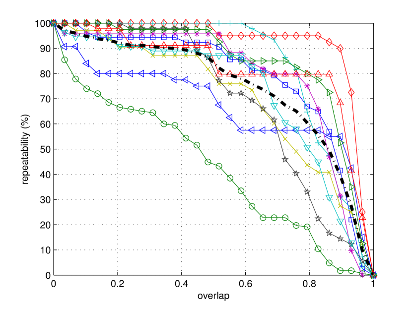
6.2 Region feature detectors.
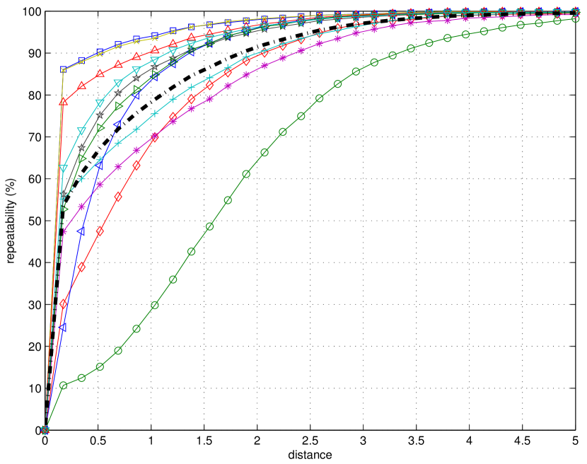
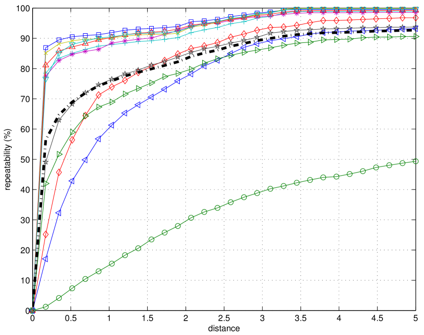
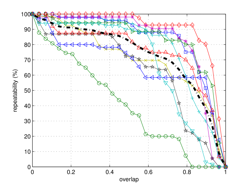
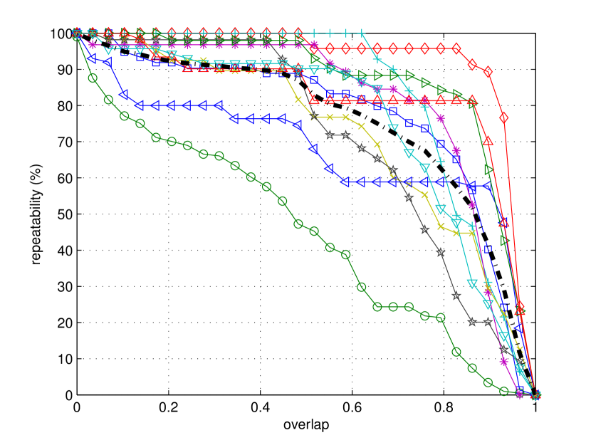
Tables 10–12 show the repeatability of different point descriptors at fixed overlap of , broken down according to transformation classes and strengths. Figure 4 shows the repeatability of region feature detectors as function of overlap varying from to .
| Strength | |||||
|---|---|---|---|---|---|
| Transform. | 1 | 2 | 3 | 4 | 5 |
| Isometry | 100.00 | 100.00 | 96.30 | 94.72 | 95.78 |
| Rasterization | 46.67 | 64.24 | 66.64 | 61.34 | 54.53 |
| Sampling | 100.00 | 100.00 | 98.15 | 73.61 | 58.89 |
| Holes | 90.00 | 45.00 | 30.00 | 22.50 | 24.34 |
| Micro holes | 100.00 | 100.00 | 100.00 | 96.15 | 84.07 |
| Scaling | 87.50 | 87.50 | 89.29 | 86.96 | 88.32 |
| Affine | 93.33 | 90.42 | 78.46 | 76.70 | 75.21 |
| Noise | 83.33 | 87.12 | 87.71 | 84.53 | 81.47 |
| Shot Noise | 92.86 | 90.18 | 83.45 | 82.90 | 81.32 |
| Partial | 75.00 | 77.50 | 57.73 | 62.05 | 58.21 |
| View | 20.00 | 60.00 | 61.43 | 69.51 | 67.04 |
| Average | 80.79 | 82.00 | 77.20 | 73.73 | 69.92 |
| Strength | |||||
|---|---|---|---|---|---|
| Transform. | 1 | 2 | 3 | 4 | 5 |
| Isometry | 88.89 | 94.44 | 92.13 | 94.10 | 92.78 |
| Rasterization | 77.78 | 78.17 | 78.78 | 65.91 | 56.36 |
| Sampling | 92.31 | 96.15 | 97.44 | 73.08 | 58.46 |
| Holes | 100.00 | 50.00 | 33.33 | 25.00 | 20.00 |
| Micro holes | 100.00 | 100.00 | 96.30 | 90.97 | 80.78 |
| Scaling | 14.29 | 57.14 | 71.43 | 78.57 | 82.86 |
| Affine | 90.91 | 88.31 | 87.08 | 87.81 | 88.03 |
| Noise | 88.89 | 86.11 | 90.74 | 93.06 | 90.44 |
| Shot Noise | 100.00 | 95.83 | 78.17 | 81.13 | 72.90 |
| Partial | 83.33 | 84.52 | 64.68 | 63.10 | 58.48 |
| View | 11.11 | 38.89 | 37.83 | 46.55 | 49.74 |
| Average | 77.05 | 79.05 | 75.26 | 72.66 | 68.26 |
| Strength | |||||
|---|---|---|---|---|---|
| Transform. | 1 | 2 | 3 | 4 | 5 |
| Isometry | 100.00 | 100.00 | 95.83 | 93.75 | 95.00 |
| Rasterization | 55.56 | 61.11 | 57.41 | 50.20 | 45.87 |
| Sampling | 100.00 | 100.00 | 95.83 | 71.88 | 57.50 |
| Holes | 87.50 | 43.75 | 29.17 | 21.88 | 22.79 |
| Micro holes | 100.00 | 100.00 | 100.00 | 96.88 | 86.39 |
| Scaling | 87.50 | 87.50 | 87.50 | 84.38 | 85.00 |
| Affine | 87.50 | 87.50 | 76.52 | 72.39 | 75.41 |
| Noise | 87.50 | 87.50 | 87.50 | 82.29 | 79.83 |
| Shot Noise | 87.50 | 82.64 | 81.02 | 80.21 | 79.72 |
| Partial | 75.00 | 75.00 | 59.52 | 63.39 | 54.05 |
| View | 12.50 | 56.25 | 55.68 | 64.26 | 60.50 |
| Average | 80.05 | 80.11 | 75.09 | 71.04 | 67.46 |
 |
 |
| Shape MSER (EW 1/CT) | Shape MSER (EW 1/HKS) |
 |
|
| Shape MSER (VW HKS) | |
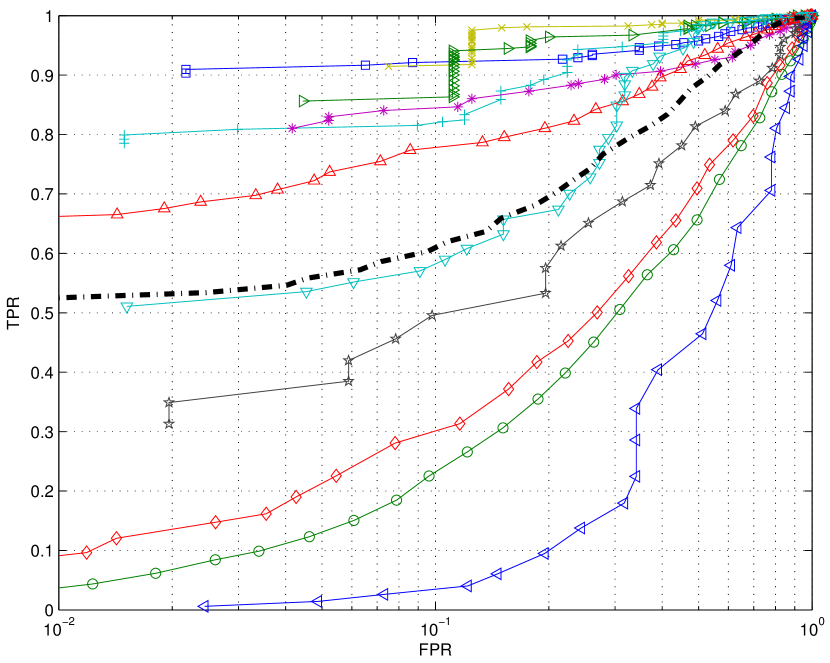
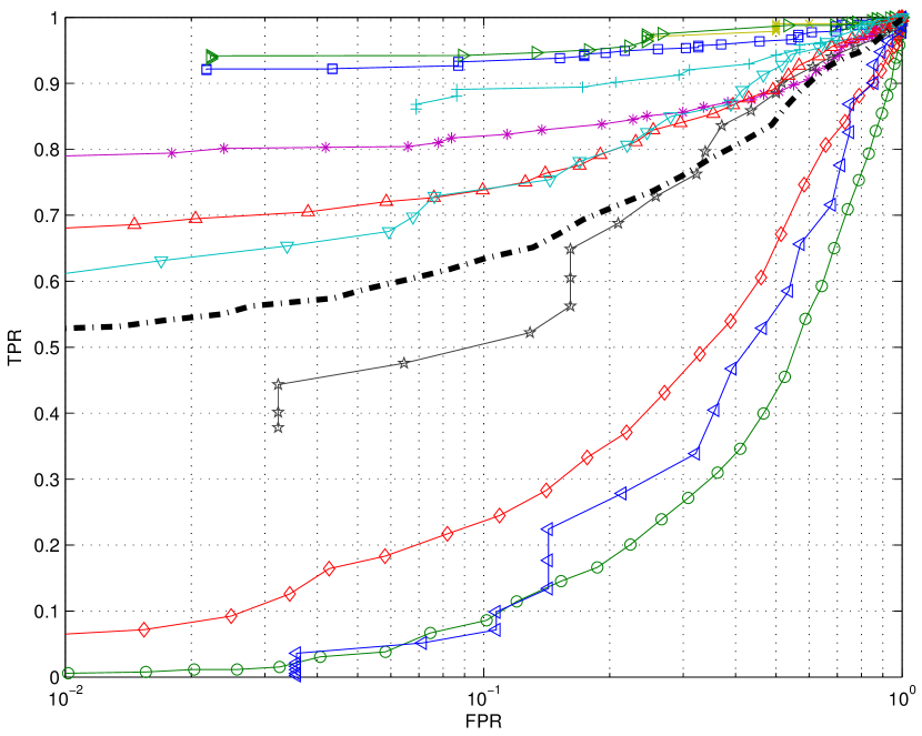
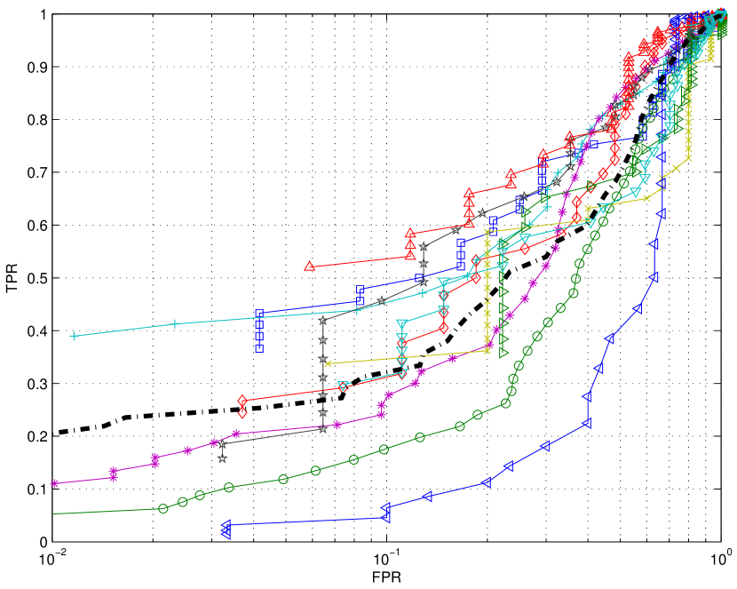
6.3 Point feature descriptors
Tables 13–18 show the performance of different point feature description algorithms, in terms of average normalized distance between corresponding descriptors. Smaller numbers correspond to better performance. Figure 5 shows the ROC curves of different point feature descriptors, using a fixed value of . Higher values of the vertical axis at a fixed point on the horizontal axis are indication of better performance.
| Strength | |||||
|---|---|---|---|---|---|
| Transform. | 1 | 2 | 3 | 4 | 5 |
| Isometry | 0.17 | 0.17 | 0.19 | 0.19 | 0.21 |
| Rasterization | 1.00 | 1.00 | 0.99 | 0.99 | 0.99 |
| Sampling | 0.93 | 0.95 | 0.96 | 0.97 | 0.98 |
| Holes | 0.23 | 0.24 | 0.26 | 0.29 | 0.32 |
| Micro holes | 0.30 | 0.31 | 0.33 | 0.34 | 0.35 |
| Scaling | 0.20 | 0.20 | 0.20 | 0.20 | 0.20 |
| Affine | 0.52 | 0.63 | 0.68 | 0.72 | 0.75 |
| Noise | 1.00 | 0.99 | 0.99 | 0.99 | 0.99 |
| Shot Noise | 0.23 | 0.24 | 0.25 | 0.26 | 0.27 |
| Partial | 0.30 | 0.36 | 0.37 | 0.46 | 0.49 |
| View | 0.64 | 0.59 | 0.61 | 0.60 | 0.60 |
| Average | 0.50 | 0.52 | 0.53 | 0.55 | 0.56 |
| Strength | |||||
|---|---|---|---|---|---|
| Transform. | 1 | 2 | 3 | 4 | 5 |
| Isometry | 0.15 | 0.15 | 0.17 | 0.17 | 0.19 |
| Rasterization | 0.98 | 0.98 | 0.99 | 0.99 | 0.99 |
| Sampling | 0.95 | 0.97 | 0.97 | 0.98 | 0.98 |
| Holes | 0.21 | 0.23 | 0.27 | 0.30 | 0.34 |
| Micro holes | 0.29 | 0.30 | 0.32 | 0.34 | 0.35 |
| Scaling | 0.19 | 0.19 | 0.19 | 0.19 | 0.19 |
| Affine | 0.58 | 0.66 | 0.71 | 0.74 | 0.78 |
| Noise | 0.98 | 0.99 | 0.99 | 0.99 | 0.99 |
| Shot Noise | 0.22 | 0.23 | 0.24 | 0.25 | 0.26 |
| Partial | 0.32 | 0.40 | 0.40 | 0.48 | 0.51 |
| View | 0.69 | 0.62 | 0.65 | 0.65 | 0.63 |
| Average | 0.51 | 0.52 | 0.54 | 0.55 | 0.56 |
| Strength | |||||
|---|---|---|---|---|---|
| Transform. | 1 | 2 | 3 | 4 | 5 |
| Isometry | 0.63 | 0.56 | 0.58 | 0.59 | 0.59 |
| Rasterization | 0.94 | 0.94 | 0.94 | 0.94 | 0.94 |
| Sampling | 0.74 | 0.77 | 0.81 | 0.84 | 0.87 |
| Holes | 0.71 | 0.73 | 0.75 | 0.77 | 0.78 |
| Micro holes | 0.70 | 0.74 | 0.76 | 0.78 | 0.80 |
| Scaling | 0.68 | 0.70 | 0.72 | 0.74 | 0.75 |
| Affine | 0.87 | 0.88 | 0.90 | 0.91 | 0.93 |
| Noise | 0.95 | 0.96 | 0.97 | 0.98 | 0.98 |
| Shot Noise | 0.70 | 0.73 | 0.76 | 0.78 | 0.80 |
| Partial | 0.46 | 0.47 | 0.53 | 0.57 | 0.59 |
| View | 0.76 | 0.74 | 0.75 | 0.74 | 0.74 |
| Average | 0.74 | 0.75 | 0.77 | 0.79 | 0.80 |
| Strength | |||||
|---|---|---|---|---|---|
| Transform. | 1 | 2 | 3 | 4 | 5 |
| Isometry | 0.67 | 0.61 | 0.64 | 0.65 | 0.64 |
| Rasterization | 0.95 | 0.96 | 0.96 | 0.96 | 0.96 |
| Sampling | 0.79 | 0.81 | 0.85 | 0.87 | 0.90 |
| Holes | 0.79 | 0.82 | 0.84 | 0.86 | 0.87 |
| Micro holes | 0.78 | 0.80 | 0.83 | 0.84 | 0.86 |
| Scaling | 0.71 | 0.72 | 0.74 | 0.75 | 0.76 |
| Affine | 0.89 | 0.89 | 0.91 | 0.92 | 0.94 |
| Noise | 0.95 | 0.96 | 0.97 | 0.98 | 0.98 |
| Shot Noise | 0.79 | 0.81 | 0.82 | 0.83 | 0.84 |
| Partial | 0.50 | 0.51 | 0.57 | 0.61 | 0.63 |
| View | 0.84 | 0.82 | 0.83 | 0.83 | 0.83 |
| Average | 0.79 | 0.79 | 0.81 | 0.83 | 0.84 |
| Strength | |||||
|---|---|---|---|---|---|
| Transform. | 1 | 2 | 3 | 4 | 5 |
| Isometry | 0.26 | 0.52 | 0.61 | 0.52 | 0.57 |
| Rasterization | 0.88 | 0.87 | 0.87 | 0.87 | 0.87 |
| Sampling | 0.62 | 0.66 | 0.70 | 0.75 | 0.79 |
| Holes | 0.36 | 0.39 | 0.42 | 0.45 | 0.47 |
| Micro holes | 0.84 | 0.85 | 0.86 | 0.87 | 0.87 |
| Scaling | 0.24 | 0.24 | 0.24 | 0.24 | 0.24 |
| Affine | 0.60 | 0.74 | 0.75 | 0.76 | 0.79 |
| Noise | 0.96 | 0.97 | 0.98 | 0.98 | 0.99 |
| Shot Noise | 0.41 | 0.48 | 0.52 | 0.56 | 0.60 |
| Partial | 0.78 | 0.77 | 0.78 | 0.69 | 0.62 |
| View | 0.50 | 0.45 | 0.46 | 0.46 | 0.45 |
| Average | 0.58 | 0.63 | 0.65 | 0.65 | 0.66 |
| Strength | |||||
|---|---|---|---|---|---|
| Transform. | 1 | 2 | 3 | 4 | 5 |
| Isometry | 0.29 | 0.55 | 0.64 | 0.55 | 0.60 |
| Rasterization | 0.91 | 0.90 | 0.89 | 0.89 | 0.90 |
| Sampling | 0.67 | 0.71 | 0.74 | 0.78 | 0.82 |
| Holes | 0.50 | 0.55 | 0.59 | 0.62 | 0.65 |
| Micro holes | 0.89 | 0.90 | 0.90 | 0.91 | 0.92 |
| Scaling | 0.26 | 0.26 | 0.26 | 0.26 | 0.26 |
| Affine | 0.64 | 0.77 | 0.77 | 0.78 | 0.81 |
| Noise | 0.93 | 0.95 | 0.96 | 0.96 | 0.97 |
| Shot Noise | 0.51 | 0.55 | 0.58 | 0.60 | 0.62 |
| Partial | 0.80 | 0.80 | 0.80 | 0.72 | 0.66 |
| View | 0.63 | 0.58 | 0.60 | 0.59 | 0.59 |
| Average | 0.64 | 0.68 | 0.70 | 0.70 | 0.71 |
 |
 |
| Mesh HoG (mean) | Mesh HoG (2) |
 |
 |
| Local depth SIFT (1) | Local depth SIFT (2) |
 |
 |
| Scale invariant Spin Image (1) | Scale invariant Spin Image (2) |
6.4 Dense feature descriptors
Table 19 shows the performance of the GHKS dense feature description algorithm, in terms of normalized average distance between corresponding descriptors. Some results could not be computed by the participants.
| Strength | |||||
|---|---|---|---|---|---|
| Transform. | 1 | 2 | 3 | 4 | 5 |
| Isometry | 0.57 | 0.58 | 0.62 | 0.62 | 0.65 |
| Rasterization | – | – | – | – | – |
| Sampling | 0.73 | 0.74 | 0.86 | 0.94 | 0.92 |
| Holes | – | – | – | – | – |
| Micro holes | – | – | – | – | – |
| Scaling | 0.62 | 0.61 | 0.65 | 0.65 | 0.75 |
| Affine | 1.08 | 1.32 | 1.46 | 1.61 | 1.77 |
| Noise | 3.24 | 3.37 | 3.37 | 3.34 | 3.32 |
| Shot Noise | 0.89 | 1.03 | 1.21 | 1.33 | 1.40 |
| Partial | 0.80 | 0.97 | 1.12 | 1.10 | 1.15 |
| View | – | – | – | – | – |
References
- [BBB∗11] Boyer E., Bronstein A. M., Bronstein M. M., Bustos B., Darom T., Horaud R., Hotz I., Keller Y., Keustermans J., Kovnatsky A., Litman R., Reininghaus J., Sipiran I., Smeets D., Suetens P., Vandermeulen D., Zaharescu A., Zobel V.: SHREC 2011: robust feature detection and description benchmark. In Proc. 3DOR (20011).
- [BBK08] Bronstein A. M., Bronstein M. M., Kimmel R.: Numerical geometry of non-rigid shapes. Springer, 2008.
- [DK11] Darom T., Keller Y.: Scale invariant features for 3d mesh models.
- [HS88] Harris C., Stephens M.: A combined corner and edge detection. In Proc. of The Fourth Alvey Vision Conference (1988), pp. 147–151.
- [JH99] Johnson A. E., Hebert M.: Using spin images for efficient object recognition in cluttered 3d scenes. IEEE Trans. Pattern Anal. Mach. Intell. 21, 5 (1999), 433–449.
- [LBB10] Litman R., Bronstein A., Bronstein M.: Diffusion-geometric maximally stable component detection in deformable shapes. Arxiv preprint arXiv:1012.3951 (2010).
- [Low04] Lowe D.: Distinctive image features from scale-invariant keypoints. IJCV 60, 2 (2004), 91–110.
- [MCUP04] Matas J., Chum O., Urban M., Pajdla T.: Robust wide-baseline stereo from maximally stable extremal regions. Image and Vision Computing 22, 10 (2004), 761–767.
- [MDSB02] Meyer M., Desbrun M., Schröder P., Barr A. H.: Discrete differential geometry operators for triangulated 2-dimensional manifolds. In Proceedings of VisMath (2002).
- [MFK∗10] Maes C., Fabry T., Keustermans J., Smeets D., Suetens P., Vandermeulen D.: Feature detection on 3D face surfaces for pose normalisation and recognition. In Proc. BTAS (2010).
- [MS05] Mikolajczyk K., Schmid C.: A performance evaluation of local descriptors. Trans. PAMI (2005), 1615–1630.
- [SB10] Sipiran I., Bustos B.: A robust 3D interest points detector based on Harris operator. In Proc. Eurographics Workshop on 3D Object Retrieval (2010), Eurographics Association, pp. 7–14.
- [SOG09] Sun J., Ovsjanikov M., Guibas L.: A concise and provably informative multi-scale signature based on heat diffusion. In Eurographics Symposium on Geometry Processing (SGP) (2009).
- [SZ03] Sivic J., Zisserman A.: Video Google: A text retrieval approach to object matching in videos. In Proc. ICCV (2003), vol. 2, pp. 1470–1477.
- [ZBVH09] Zaharescu A., Boyer E., Varanasi K., Horaud R.: Surface feature detection and description with applications to mesh matching.
- [Zob10] Zobel V.: Spectral Analysis of the Hodge Laplacian on Discrete Manifolds. Master Thesis, 2010.
- [ZRHar] Zobel V., Reininghaus J., Hotz I.: Generalized heat kernel signature. Journal of WSCG, International Conference on Computer Graphics, Visualization and Computer Vision (2011 to appear).