Wavelets centered on a knot sequence: theory, construction, and applications

Abstract.

We develop a general notion of orthogonal wavelets ‘centered’ on an irregular knot sequence. We present two families of orthogonal wavelets that are continuous and piecewise polynomial. We develop efficient algorithms to implement these schemes and apply them to a data set extracted from an ocelot image. As another application, we construct continuous, piecewise quadratic, orthogonal wavelet bases on the quasi-crystal lattice consisting of the $\tau$-integers where $\tau$ is the golden ratio. The resulting spaces then generate a multiresolution analysis of $L^{2}(\mathbf{R})$ with scaling factor $\tau$.

Introduction

Wavelets are a useful tool for representing general functions and datasets and are now used in a wide variety of areas such as signal processing, image compression, function approximation, and finite-element methods. Traditionally wavelets are constructed from one function, the so-called mother wavelet, by integer translation and dyadic dilation and give rise to a stationary refinement equation. For many functions however this may not be the most efficient way of approximating them and one may require adaptive schemes for which the knot sequence is not regularly spaced or where the knots are on a regular grid but the refinement equation changes at each step. There has been much work devoted to extending wavelet constructions to irregularly spaced knot sequences including the lifting scheme of Sweldens [27] and wavelets on irregular grids (see Daubechies et. al. [11],[12], Charina and Stöckler [5]) or nonstationary tight wavelet frames (see Chui, He, and Stöckler, [6, 7] and Shah [26]) or to nonstationary refinement masks (see Cohen and Dyn [9] and Herley, Kovac̆ević, and Vetterli [21]). If the knots are allowed to be chosen generally enough it is difficult to maintain the orthogonality of the wavelet functions while keeping the compact support and smoothness properties.

In [13, 16] piecewise polynomial, orthogonal, multiwavelets with compact support were constructed using multiresolution analyses that were intertwined with classical spline spaces. Both the multiwavelets as well as the scaling functions generating these multiwavelets have ‘short’ support allowing them to be adapted to irregular knot sequences using the machinery of squeezable bases developed in [14, 15] in a way that preserved the orthogonality, polynomial reproduction, and smoothness of the respective bases. In general, the multiresolution analyses were restricted to semi-regular refinement schemes in which an initial irregular knot sequence is refined by a regular refinement scheme such as mid-point subdivision (cf. [4]). However, in [15], a construction was given of a fully irregular multiresolution analysis consisting of continuous, piecewise quadratic functions on an arbitrary sequence of nested knot sequences such that the multiresolution spaces have compactly supported orthogonal bases with ‘short’ support (we review and generalize this construction in Section 1.4). The resulting spaces in the multiresolution analysis did not fit, for general knot sequences, into the framework of squeezable bases. In [3], a more general notion of bases centered on a knot sequence was introduced that includes the squeezable bases as well as the irregular construction. In particular, necessary and sufficient conditions were given for when a space $V$ has an orthogonal basis centered on a knot sequence. This is used to prove one of the main results of this paper that if $V^{0}\subset V^{1}$ are spaces generated by orthogonal bases centered on a common knot sequence $\mathbf{a}$ then the orthogonal complement $W=V^{1}\ominus V^{0}$ is also generated by an orthogonal basis $\Psi$ centered on $\mathbf{a}$.

In Section 1 we review and further elucidate the theory of bases centered on a knot sequence. In particular, as mentioned above, we focus on the question of characterizing spaces that are generated by orthogonal bases centered on a knot sequence. We next give two different constructions of nested spaces of this type. The first uses a fixed knot sequence $\mathbf{a}$ and constructs $V^{0}\subset V^{1}\subset\cdots$ which are spaces generated by orthogonal continuous piecewise polynomial functions with compact support and with breakpoints in $\mathbf{a}$; these spaces have increasing polynomial reproduction. The second construction begins with a given knot sequence $\mathbf{a}$ and the spline space $S^{0}_{2}(\mathbf{a})$ consisting of continuous piecewise quadratic functions with breakpoints in $\mathbf{a}$. The knot sequence $\mathbf{a}$ is then refined and a space $V$, containing $S^{0}_{2}(\mathbf{a})$, is constructed which is generated by continuous orthogonal piecewise quadratic functions with compact support and breakpoints in the refined sequence. If $\mathbf{a^{0}}\subset\mathbf{a^{1}}$ and $V^{0}$ (resp. $V^{1}$) is constructed in this way starting with $\mathbf{a^{0}}$ (resp. $\mathbf{a^{1}}$), we describe general conditions under which $V^{0}\subset V^{1}$.

In Section 2 it is shown how to build wavelets from the scaling functions constructed in the previous section. Certain spaces are introduced which shed light on techniques of [16]. The wavelet construction methods given in [16] are sufficiently general so that they can be used to give a decomposition of the wavelet spaces, thus providing a convenient algorithm for calculating these bases.

In Section 3 efficient algorithms are developed in order to demonstrate practicality of the method developed in the previous sections. The matrices, defined in section 2, in the equations for the scaling functions and wavelets are computed after a knot is added or dropped. These algorithms are based upon the greedy algorithm and nonlinear approximation schemes [1], [9], [17] and an application to a data set extracted from the digital image of an ocelot is given to show their effectiveness.

In Section 4 a construction of multiwavelets is carried out for the knot sequence consisting of the $\tau$-integers, where $\tau=\frac{1}{2}(1+\sqrt{5})$ is the golden mean. These multiwavelets have a scaling factor $\tau$ and will be called $\tau$-multiwavelets. The lattice generated by $\tau$ and other Pisot numbers appears in the study of quasi-crystals and powers of these numbers appear in the diffraction patterns of actual experiments. $\tau$-Haar wavelets were constructed in [19, 20]. $\tau$-Haar wavelets are orthogonal and compactly supported but they are not continuous. The above construction is used to give examples of piecewise quadratic continuous compactly supported $\tau$-multiwavelets. Additional work on multiresolution analyses with irrational scaling factors includes Chui and Shi [8], Hernández, Wang, and Weiss [22], [23], and Bownik [2].

1. Bases Centered on Knot Sequences

Let $J$ be an interval in $\mathbf{R}$ and let $\mathbf{a}\subset J$ have no cluster point in $J$ and such that $\inf\mathbf{a}=\inf J$ and $\sup\mathbf{a}=\sup J$; to avoid trivial cases we assume that $\mathbf{a}$ consists of at least three elements. We refer to such a set $\mathbf{a}$ as a knot sequence in $J$ since it can be represented as the range of a strictly increasing sequence indexed by an interval $\mathcal{I}\subset\mathbf{Z}$.

Let $\mathbf{a}$ be a knot sequence in $J$. If $a\in\mathbf{a}$, we define $a_{+}:=\inf\{b\in\mathbf{a}|a<b\}$; in this case we shall refer to $a_{+}$ as the successor of $a$ in $\mathbf{a}$. We will write $a_{++}$ for $(a_{+})_{+}$. Similarly, we define $a_{-}:=\sup\{b\in\mathbf{a}|b<a\}$; i.e. $a_{-}$ is the predecessor of $a$ in $\mathbf{a}$. We remark that $a_{+}=\infty$ if $a=\sup J$ and $a_{-}=-\infty$ if $a=\inf J$.

For an arbitrary collection of functions $G\subset L^{2}(J)$ and an interval $I\subset J$, let

$$G_{I}:=\{g\in G\ |\ \text{supp }g\subset I\}.$$

If $\Phi\subset L^{2}(J)$ is a locally finite collection of functions (i.e., on any compact interval $K\subset J$ all but a finite number of $\phi\in\Phi$ vanish on $K$) then for $a\in\mathbf{a}$ we define

(1) $$\begin{split}\breve{\Phi}_{a}&:=\Phi_{[a,a_{+}]},\\ \Phi_{a}&:=\Phi_{[a_{-},a_{+}]}\setminus\breve{\Phi}_{a_{-}},\text{ and}\\ \bar{\Phi}_{a}&:=\Phi_{a}\setminus\breve{\Phi}_{a},\end{split}$$

where we define $\breve{\Phi}_{-\infty}:=\emptyset$ and $\bar{\Phi}_{\infty}:=\emptyset$. We remark that if $J$ contains its supremum and $a=\sup J$ then $\Phi_{a}=\emptyset$ while if $J$ contains its infimum and $a=\inf J$ then $\bar{\Phi}_{a}=\emptyset$. The sets $\breve{\Phi}_{a}$, $\bar{\Phi}_{a}$, and $\Phi_{a}$ depend on the knot sequence ${\mathbf{a}}$ since $a_{+}$ and $a_{-}$ are defined relative to $\mathbf{a}$. When there is a chance of ambiguity we write $\breve{\Phi}_{a,\mathbf{a}}$, $\bar{\Phi}_{a,\mathbf{a}}$, and $\Phi_{a,\mathbf{a}}$ to denote the knot sequence $\mathbf{a}$ that is referenced.

We say that $\Phi\subset L^{2}(J)$ is a basis  centered on the knot sequence $\mathbf{a}$ provided

(2) $$\begin{split}\text{(a) }&\text{$\Phi$ is locally finite,}\\ \text{(b) }&\text{ $\Phi=\bigcup_{a\in\mathbf{a}}\Phi_{a}$, and}\\ \text{(c) }&\text{ $\left(\Phi_{a}\cup\bar{\Phi}_{a_{+}}\right)|_{[a,a_{+}]}$ is a linearly independent set for all $a\in\mathbf{a}$}.\end{split}$$

For any $\Phi$ satisfying conditions (a) and (b) of (2), we let

$$S(\Phi):=\text{clos}_{L^{2}(J)}\text{span }(\Phi).$$

The notion of a basis centered on a knot sequence was introduced in [3] and is a generalization of bases obtained from minimally supported generators as defined in [13, 15]. Roughly speaking, a basis centered on a knot sequence consists of functions whose supports overlap at most on a single ‘knot interval’ and the non-zero restrictions of these functions to each such knot interval are linearly independent.

If $\Phi$ is a basis centered on $\mathbf{a}$ then it follows from properties (2) that any $f\in S(\Phi)$ has a unique representation of the form

(3) $$f=\sum_{a\in\mathbf{a}}c_{a}\Phi_{a}=\sum_{a\in\mathbf{a}}(\breve{c}_{a}\breve{\Phi}_{a}+\bar{c}_{a}\bar{\Phi}_{a}),$$

where the convergence of the sums is in $L^{2}_{\textrm{loc}}(J)$. Note that $c_{a}$, $\breve{c}_{a}$, and $\bar{c}_{a}$ are treated as row vectors and $\Phi_{a}$, $\breve{\Phi}_{a}$, and $\bar{\Phi}_{a}$ are treated as column vectors so that $c_{a}\Phi_{a}$ denotes the linear combination of elements $\Phi_{a}$ with coefficient vector $c_{a}$; the expressions $\breve{c}_{a}\breve{\Phi}_{a}$ and $\bar{c}_{a}\bar{\Phi}_{a}$ are interpreted similarly. It then follows from the local linear independence condition (c) that

(4) $$\text{ $f\in S(\Phi)$ and $f=0$ on $[a,a_{+}]$}\implies\text{ $\bar{c}_{a}$, $\bar{c}_{a_{+}}$ and $\breve{c}_{a}$ are all 0},$$

and then (4) implies

(5) $$S(\Phi)_{[a,b]}=\text{ span }\left(\Phi_{[a,b]}\right)=\text{ span }(\breve{\Phi}_{a}\cup(\bigcup_{\begin{subarray}{c}c\in\mathbf{a}\\ a<c<b\end{subarray}}\,\Phi_{c})),$$

for $a,b\in\mathbf{a}$ with $a<b$. Note that if there are no knots $c$ between $a$ and $b$, then the sum (resp. union) in equation (5) is zero (resp. empty).

For $V\subset L^{2}(J)$, let

$$V_{a}:=V_{[a_{-},a_{+}]}\text{ and }\breve{V}_{a}:=V_{[a,a_{+}]}\qquad a\in\mathbf{a}.$$

Note that if $\Phi$ is a basis centered on the knot sequence $\mathbf{a}$ and $V=S(\Phi)$, then equation (5) implies that for $a\in\mathbf{a}$,

$$\breve{V}_{a}=\text{span }\breve{\Phi}_{a}$$

and

$$V_{a}=\text{span (}\breve{\Phi}_{a_{-}}\cup\Phi_{a}).$$

In particular it follows that each $V_{a}$ is finite dimensional. We next characterize when $V\subset L^{2}(J)$ equals $S(\Phi)$ for some basis $\Phi$ centered on $\mathbf{a}$.

Theorem 1.

Let $\mathbf{a}$ be a knot sequence in an interval $J$ and suppose $V\subset L^{2}(J)$. Then $V=S(\Phi)$ for some basis $\Phi$ centered on $\mathbf{a}$ if and only if the following three properties hold.

• $V_{a}$ is a finite dimensional subspace of $L^{2}(J)$ for $a\in\mathbf{a}$.

• $V=\text{clos}_{L^{2}(J)}\text{ span }\left(\bigcup_{a\in\mathbf{a}}V_{a}\right).$

• If $f\in V$ vanishes on $[a,a_{+}]$, then $f\in V_{(-\infty,a]}+V_{[a_{+},\infty)}$.

If ($\hat{a}$–$\hat{c}$) hold, then, for $a\in\mathbf{a}$, let $\breve{\Phi}_{a}$ be a basis for $\breve{V}_{a}$ and let $\bar{\Phi}_{a}$ augment $\breve{\Phi}_{a_{-}}\cup\breve{\Phi}_{a}$ to a basis of $V_{a}$. Then $\Phi:=\bigcup_{a\in\mathbf{a}}\left(\bar{\Phi}_{a}\cup\breve{\Phi}_{a}\right)$ is a basis centered on $\mathbf{a}$ such that $V=S(\Phi).$ Furthermore, any $\Phi$ such that $V=S(\Phi)$ is of this form, that is, $\breve{\Phi}_{a}$ must be a basis of $\breve{V}_{a}$ and $\bar{\Phi}_{a}\cup\breve{\Phi}_{a_{-}}\cup\breve{\Phi}_{a}$ must be a basis of $V_{a}$.

Remark 1.

Theorem 1 implies that if $\Phi$ is a basis centered on a knot sequence $\mathbf{b}$ that is a refinement of $\mathbf{a}$ (i.e., $\mathbf{a}\subset\mathbf{b}$), then $\Phi$ is also a basis centered on $\mathbf{a}$. Note that, for $a\in\mathbf{a}\subset\mathbf{b}$, the sets $\Phi_{a,\mathbf{a}}$ and $\Phi_{a,\mathbf{b}}$ are, in general, not equal.

Proof.

($\Rightarrow$) Suppose $V=S(\Phi)$ for some basis $\Phi$ centered on the knot sequence $\mathbf{a}$. Conditions ($\hat{a}$) and ($\hat{b}$) then follow from (5) and condition ($\hat{c}$) follows from (4).

($\Leftarrow$) Suppose that ($\hat{a}$–$\hat{c}$) hold and that $\breve{\Phi}_{a}$ and $\bar{\Phi}_{a}$ are constructed as in the statement of Theorem 1. Then ($\hat{b}$) implies $V=S(\Phi)$ and so it remains to show the local linear independence condition of $\Phi$. Let $a\in\mathbf{a}$ and suppose that $\bar{c}_{a}$, $\breve{c}_{a}$, and $\breve{c}_{a_{+}}$ are vectors so that

(6) $$f:=\bar{c}_{a}\bar{\Phi}_{a}+\breve{c}_{a}\breve{\Phi}_{a}+\bar{c}_{a_{+}}\bar{\Phi}_{a_{+}}=0\text{ on $[a,a_{+}]$.}$$

It now suffices to show that these coefficient vectors must all vanish. By condition ($\hat{c}$), we have $f=f_{1}+f_{2}$ where $f_{1}\in V_{(-\infty,a]}$ and $f_{2}\in V_{[a_{+},\infty)}$. Since $f$ and $f_{2}$ vanish on $(-\infty,a_{-}]$ it follows that $f_{1}\in V_{[a_{-},a]}$. Hence, $f_{1}=\breve{d}_{a_{-}}\breve{\Phi}_{a_{-}}$ for some vector $\breve{d}_{a_{-}}$ by the construction of $\breve{\Phi}_{a_{-}}$. Then $g:=\bar{c}_{a}\bar{\Phi}_{a}-\breve{d}_{a_{-}}\breve{\Phi}_{a_{-}}=0$ on $[a_{-},a]$. Since the support of $g$ is in $[a,a_{+}]$, then $g=\breve{d}_{a}\breve{\Phi}_{a}$ for some vector $\breve{d}_{a}$, i.e.,

$$\bar{c}_{a}\bar{\Phi}_{a}-\breve{d}_{a_{-}}\breve{\Phi}_{a_{-}}-\breve{d}_{a}\breve{\Phi}_{a}=0.$$

Since $\bar{\Phi}_{a}$, $\breve{\Phi}_{a_{-}}$ and $\breve{\Phi}_{a}$ are linearly independent, it follows that $\bar{c}_{a}=0$. Similarly, we have $\bar{c}_{a_{+}}=0$ and thus, by the linear independence of $\breve{\Phi}_{a}$ we have $\breve{c}_{a}=0$. ∎

1.1. Example

Let $\Pi^{d}$ denote the space of univariate polynomials of degree at most $d$. For a knot sequence $\mathbf{a}$ on an interval $J$ and integers $r<d$, let

$$S_{d}^{r}(\mathbf{a}):=\{f\mid\text{supp }f\subset J,\,f\in C^{r}(J)\cap L^{2}(J),\text{ and }f|_{(a,a_{+})}\in\Pi^{d}\text{ for }a\in\mathbf{a}\}$$

denote the classical spline space of degree $d$ and regularity $r$ intersected with $L^{2}(J)$. If $d\geq 2r+1$, then $S_{d}^{r}(\mathbf{a})=S(\Phi)$ for a basis $\Phi$ centered on $\mathbf{a}$. For example, the B-spline basis for $S_{d}^{r}(\mathbf{a})$, which we denote by $\Phi_{r,d}^{\mathbf{a}}$, is such a basis, cf. [25]. Furthermore, $|\breve{\Phi}_{a}|=d-2r-1$ if $a<\sup J$, and for $\inf J<a<\sup J$, we have $|\Phi_{a}|=d-r$ and $|\bar{\Phi}_{a}|=r+1$.

1.2. Orthogonality Condition

Bases $\Phi$ and $\Psi$ centered on the same knot sequence $\mathbf{a}$ in the interval $J$ are called equivalent if $S(\Phi)=S(\Psi)$. We next give a necessary and sufficient condition for a basis $\Phi$ centered on $\mathbf{a}$ to be equivalent to some orthogonal basis $\Omega$ centered on $\mathbf{a}$. This condition is the main tool we use to construct orthogonal bases centered on a knot sequence. Previous versions of this theorem appeared in [13] (for the shift-invariant setting), in [15] (for the setting of “squeezable” orthogonal bases) and in [3] (for the current setting of bases centered on a knot sequence).

Theorem 2.

Let $J$ be an interval in $\mathbf{R}$, $\mathbf{a}$ a knot sequence on $J$, $\Phi$ a basis centered on $\mathbf{a}$, and $V=S(\Phi)$. Then there exists an orthogonal basis $\Omega$ centered on the knot sequence $\mathbf{a}$ such that $S(\Omega)=S(\Phi)$ if and only if

(7) $$\left(I-P_{\breve{V}_{a}}\right)V_{a}\perp V_{a_{+}}\text{ for }a\in\mathbf{a}\text{.}$$

If (7) holds, then, for $a\in\mathbf{a}$, let $\breve{\Omega}_{a}$ be an orthogonal basis of $\breve{V}_{a}$, $\bar{\Omega}_{a}$ be an orthogonal basis of $\left(I-P_{\breve{V}_{a_{-}}\oplus\breve{V}_{a}}\right)V_{a}$, and $\Omega_{a}=\breve{\Omega}_{a}\cup\bar{\Omega}_{a}$. Then $\Omega=\{\Omega_{a}\}_{a\in\mathbf{a}}$ is such an orthogonal basis.

Proof.

Suppose $a\in\mathbf{a}$. Note that $\breve{V}_{a_{-}}\perp V_{a_{+}}$ since their supports intersect in at most one point. It then follows that (7) is equivalent to

$$\left(I-P_{\breve{V}_{a_{-}}\oplus\breve{V}_{a}}\right)V_{a}\perp V_{a_{+}}\text{.}$$

Furthermore, since $\left(I-P_{\breve{V}_{a_{-}}\oplus\breve{V}_{a}}\right)V_{a}$ is orthogonal to $\breve{V}_{a}$ and, due to support properties, is also orthogonal to $\breve{V}_{a_{+}}$, it follows that (7) is equivalent to

(8) $$\left(I-P_{\breve{V}_{a_{-}}\oplus\breve{V}_{a}}\right)V_{a}\perp\left(I-P_{\breve{V}_{a}\oplus\breve{V}_{a_{+}}}\right)V_{a_{+}}\text{.}$$

($\Rightarrow$) Suppose that $V=S(\Omega)$, where $\Omega$ is an orthogonal basis centered on the knot sequence $\mathbf{a}$. It follows from (5) and the orthogonality of $\Omega$ that

$$V_{a}=\text{span }\breve{\Omega}_{a_{-}}\oplus\text{span }\bar{\Omega}_{a}\oplus\text{span }\breve{\Omega}_{a}=\breve{V}_{a_{-}}\oplus\text{span }\bar{\Omega}_{a}\oplus\breve{V}_{a},$$

and so $\text{span}(\bar{\Omega}_{a})=\left(I-P_{\breve{V}_{a_{-}}\oplus\breve{V}_{a}}\right)V_{a}$. Since $\Omega$ is an orthogonal basis, $\text{span}(\bar{\Omega}_{a})\perp\text{span}(\bar{\Omega}_{a_{+}})$, and so (8), and hence (7), holds.

($\Leftarrow$) Suppose that $V$ satisfies (7), and hence satisfies (8). Construct $\Omega$ as in the statement of Theorem 2. By Theorem 1, it follows that $\Omega$ is a basis centered on $\mathbf{a}$ such that $V=S(\Omega)$. Equation (8) implies that $\bar{\Omega}_{a}\perp\bar{\Omega}_{a_{+}}$ for $a\in\mathbf{a}$, which shows $\Omega$ is an orthogonal basis of $V$. ∎

Suppose $V=S(\Phi)$ for some $\Phi$. Then it is easy to verify that (7) holds if and only if

(9) $$\left(I-P_{\breve{V}_{a}}\right)\bar{\Phi}_{a}\perp\bar{\Phi}_{a_{+}},\qquad a\in\mathbf{a}\text{.}$$

We use this equation as the basis for a construction of orthogonal bases centered on a knot sequence as we next describe. Suppose

$$Z:=\text{clos}_{L^{2}(J)}\text{span }\big{(}\bigcup_{a\in\mathbf{a}}Z_{a}\big{)},$$

where $Z_{a}$, $a\in\mathbf{a}$ is a finite dimensional subspace of $L^{2}(J)$ such that (a) the elements of $Z_{a}$ are supported in $[a,a_{+}]$ and (b) $Z_{a}$ is linearly independent of $V$ restricted to $[a,a_{+}]$. Then $U:=V+Z$ satisfies the hypotheses ($\hat{a}$), ($\hat{b}$), and ($\hat{c}$) of Theorem 1 and, by this lemma, $U=S(\Theta)$ where $\Theta$ is a basis centered on $\mathbf{a}$ such that $\breve{\Theta}_{a}$ is a basis for $\breve{U}_{a}=\breve{V}_{a}+Z_{a}$ and $\bar{\Theta}_{a}:=\bar{\Phi}_{a}$ for $a\in\mathbf{a}$. By Theorem 2, $U=S(\Omega)$ for some orthogonal basis $\Omega$ centered on $\mathbf{a}$ if and only if

(10) $$\left(I-P_{\breve{V}_{a}+Z_{a}}\right)\bar{\Phi}_{a}\perp\bar{\Phi}_{a_{+}},\qquad a\in\mathbf{a}.$$

Without loss of generality, we may choose $Z_{a}$ orthogonal to $\breve{V}_{a}$. Then (10) is equivalent to

(11) $$\langle(I-P_{\breve{V}_{a}})\bar{\Phi}_{a},\bar{\Phi}_{a_{+}}\rangle=\langle P_{Z_{a}}\bar{\Phi}_{a},\bar{\Phi}_{a_{+}}\rangle,\qquad a\in\mathbf{a}.$$

where for finite collections $F,G\subset{L^{2}({\bf R})}$, we let $\langle F,G\rangle$ denote the matrix $\left(\langle f,g\rangle\right)_{f\in F,g\in G}$ indexed by $F$ and $G$. Then from (11) it follows that

$$\dim Z_{a}\geq\text{rank }\langle(I-P_{\breve{V}_{a}})\bar{\Phi}_{a},\bar{\Phi}_{a_{+}}\rangle.$$

We remark that if one finds a $Z_{a}$ that satisfies (10), then one can always choose $Z^{\prime}_{a}\subset Z_{a}$ such that equality holds in the above estimate.

In this paper, we focus on constructions in which the spaces $Z_{a}$ above are chosen via a generalization of the intertwining technique developed in [13] (and extended in [3] and [15]) to construct orthogonal piecewise polynomial wavelets. To that end, suppose $\Phi^{\prime}$ and $\Phi^{\prime\prime}$ are bases centered on $\mathbf{a}$ such that

(12) $$S(\Phi)\subset S(\Phi^{\prime})\subset S(\Phi^{\prime\prime})$$

and that there exist spaces $Z_{a}\subset$ span $\breve{\Phi}_{a}^{\prime}$ (respectively, $Z_{a}^{\prime}\subset$ span $\breve{\Phi}_{a}^{\prime\prime}$), $a\in\mathbf{a}$, as in the previous paragraph, so that there exists an orthogonal basis $\Omega$ (respectively, $\Omega^{\prime}$) such that $S(\Omega)=S(\Phi)+S(Z)$ (respectively, $S(\Omega^{\prime})=S(\Phi^{\prime})+S(Z^{\prime})$). It then follows that

$$S(\Omega)\subset S(\Phi^{\prime})\subset S(\Omega^{\prime}).$$

Specifically, suppose $\mathbf{b}$ and $\mathbf{c}$ are knot sequences in $J$ so that $\mathbf{a}\subset\mathbf{b}\subset\mathbf{c}$ and consider the spline bases $\Phi=\Phi_{r,d}^{\mathbf{a}}$, $\Phi^{\prime}=\Phi_{r,d}^{\mathbf{b}}$, and $\Phi^{\prime\prime}=\Phi_{r,d}^{\mathbf{c}}$ where $r\geq 2d+1$. Then $S(\Phi)\subset S(\Phi^{\prime})\subset S(\Phi^{\prime\prime})$. We also recall that $\Phi^{\prime}$ and $\Phi^{\prime\prime}$ are bases centered on $\mathbf{a}$ as well as centered on $\mathbf{b}$ and $\mathbf{c}$, respectively; see the remark following Theorem 1.

1.3. Continuous, orthogonal, spline basis centered on a knot sequence: arbitrary polynomial reproduction.

In this example we will use extensively the results of [16]. Let $J$ be an interval in $\mathbf{R}$, $\mathbf{a}$ a knot sequence in $J$, and let $S_{n}^{0}(\mathbf{a})$ denote the spline space consisting of continuous piecewise polynomial functions in $L^{2}(J)$ of degree at most $n$ defined on $J~{}$with break points in $\mathbf{a}$. Then $S_{n}^{0}(\mathbf{a})=S(\Phi)$ for a basis $\Phi$ centered on $\mathbf{a}$. Let $I=[0,1]$, and let $\Pi^{n}$ denote the space of polynomials of degree $n$ on $I$. If we set $\tilde{\phi}^{i}(x)=x(1-x)p_{i-2}^{\frac{5}{2}}(2x-1)\chi_{[0,1)}(x),\ i=2,3,\ldots,n$ where $p_{i}^{\frac{5}{2}}(x)$ is the monic ultraspherical polynomial of degree $i$ in $x$ then $\{\tilde{\phi}^{i}\}_{i=2}^{n}$ form an orthogonal set in $L^{2}(I)$. Let $r=x\chi_{[0,1)}(x)$, $l=(1-x)\chi_{[0,1)}(x)$,

(13) $$r_{n}=(I-P_{\{\tilde{\phi}^{k}\,|\,k=2,\ldots,n\}})r,\ \text{and}\ l_{n}=(I-P_{\{\tilde{\phi}^{k}\,|\,k=2,\ldots,n\}})l.$$

(Note: Here, and following, when $A$ is a finite set of functions, we will write $P_{A}$ to denote the more cumbersome $P_{\text{ span }A}$.)

Some useful integrals that we will need later are

(14) $$\|\tilde{\phi}^{n}\|^{2}=\frac{(n-2)!(n+2)!}{16(2n-1)!!(2n+1)!!},$$

(15) $$\langle r,\tilde{\phi}^{n}\rangle=\frac{(n-2)!}{4(2n-1)!!},\ \langle l,\tilde{\phi}^{n}\rangle=(-1)^{n}\langle r,\tilde{\phi}^{n}\rangle,$$

and

(16) $$\langle r_{n},l_{n}\rangle=(-1)^{n+1}\frac{1}{n(n+1)(n+2)}.$$

Here we use the notation that $(2n-1)!!=(2n-1)(2n-3)\cdots(1)$. These formulas may be obtained from [16] (cf., Equation 2.3 with $m=2$; Equation 2.5 with $i=0$, $k=0$; and Equation 5.3 where $\tilde{\phi}^{n}(x)=\frac{1}{4}\phi_{n}^{0}(2x-1)\chi_{[0,1)}(x)$, $r(x)=\frac{1}{2}r_{0}^{0}(2x-1)\chi_{[0,1)}(x)$ and $l(x)=\frac{1}{2}l_{0}^{0}(2x-1)\chi_{[0,1)}(x)$). Since $r_{n}$ and $l_{n}$ are not orthogonal we add a function $z^{n}$ chosen so that when it is projected out from the above two functions they become orthogonal. To accomplish this set,

(17) $$z^{n}=\alpha_{n}\tilde{\phi}^{n+1}+\tilde{\phi}^{n+3},$$

where $\alpha_{n}$ is fixed so that

(18) $$\|z^{n}\|^{2}\langle r_{n},(I-P_{\{z^{n}\}})l_{n}\rangle=\langle r_{n},l_{n}\rangle\|z^{n}\|^{2}-(-1)^{n+1}\langle r,z^{n}\rangle^{2}=0,$$

where (15) has been used to obtain the above equation. The choice of $z^{n}$ above is for simplicity and to preserve the symmetry properties of the basis being constructed. Substituting (17) into (18) and using the integrals computed above yields the quadratic equation

$$\alpha_{n}^{2}+\left(\frac{2(n+1)}{2n+5}\right)\alpha_{n}+\left(\frac{(n+2)(n+1)(n^{2}-5n-30)}{(2n+7)((2n+5)^{2}(2n+3)}\right)=0.$$

Choosing the positive square root in the quadratic formula we obtain the solution

(19) $$\alpha_{n}=-\frac{n+1}{2n+5}+\frac{n+3}{2n+5}\sqrt{\frac{3(n+1)(n+3)}{(2n+7)(2n+3)}}.$$

Now we set

$$r^{n}=(I-P_{\{\tilde{\phi}^{2},\ldots,\tilde{\phi}^{n},z^{n}\}})r=(I-P_{\{z^{n}\}})r_{n}$$

and

$$l^{n}=(I-P_{\{\tilde{\phi}^{2},\ldots,\tilde{\phi}^{n},z^{n}\}})l=(I-P_{\{z^{n}\}})l_{n}.$$

Let $\tilde{\Pi}^{n}=\text{span}\{\Pi^{n},z^{n}\}$. The above construction shows,

Lemma 3.

The functions $\{r^{n},l^{n},z^{n},\tilde{\phi}^{i}\ i=2,\ldots,n\}$ form an orthogonal basis for $\tilde{\Pi}^{n}$. Furthermore $\tilde{\Pi}^{n}\subset\tilde{\Pi}^{n+3}$.

We now construct a continuous orthogonal basis centered on $\mathbf{a}$. Let $\sigma_{a}$ be the affine function taking $a$ to 0 and $a_{+}$ to 1. For each $a<\sup J$ let $\tilde{\phi}^{n}_{a}=\tilde{\phi}^{n}\circ\sigma_{a}$, $z^{n}_{a}=z^{n}\circ\sigma_{a}$, $r^{n}_{a}=r^{n}\circ\sigma_{a}$, and $l^{n}_{a}=l^{n}\circ\sigma_{a}$. For $a<\sup J$ define

$$\breve{\Omega}^{n}_{a}=\left\{\begin{array}[c]{cc}\{l^{n}_{a},z^{n}_{a},\tilde{\phi}^{2}_{a},\ldots,\ \tilde{\phi}^{n}_{a}\}&\text{if }a=\inf J\\ \{z^{n}_{a},\tilde{\phi}^{2}_{a},\ldots,\tilde{\phi}^{n}_{a}\}&\text{if }\inf J<a<a_{+}<\sup J\\ \{r^{n}_{a},z^{n}_{a},\tilde{\phi}^{2}_{a},\ldots,\ \tilde{\phi}^{n}_{a}\}&\text{if }a_{+}=\sup J\end{array}\right.\text{.}$$

and, for $\inf J<a<\sup J$,

$$\bar{\Omega}^{n}_{a}=\{r^{n}_{a_{-}}+l^{n}_{a}\}.$$

From the above construction we see that $\breve{\Omega}^{n}_{a}$ and $\bar{\Omega}^{n}_{a}$, for $a\in\mathbf{a}$, form an orthogonal basis $\Omega^{n}_{\mathbf{a}}$ centered on the knot sequence $\mathbf{a}$ and that

(20) $$S_{n}^{0}(\mathbf{a})\subset S(\Omega^{n}_{\mathbf{a}})\subset S^{0}_{n+3}(\mathbf{a})\subset S(\Omega^{n+3}_{\mathbf{a}})$$

which implies

Proposition 4.

Let $\mathbf{a}$ be a knot sequence and, for a fixed $\kappa\in\{1,2,3\}$, let $V^{k}:=S(\Omega^{3k+\kappa}_{\mathbf{a}}),k=0,1,2,\ldots$. Then $V^{k}\subset V^{k+1}$ and $\bigcup_{k=0}^{\infty}V^{k}$ is dense in $L^{2}(\mathbf{J})$.

Proof.

The first two statements follow from equation (20). The same equation also implies that $\bigcup_{k=0}^{\infty}S_{3k+\kappa}^{0}(\mathbf{a})\subset\bigcup_{k=0}^{\infty}V^{k}$. The third statement now follows by the density of the piecewise continuous polynomials with breakpoints on $\mathbf{a}$ in $L^{2}(\mathbf{J})$. ∎

1.4. Continuous, orthogonal, piecewise quadratic, bases centered on nested knot sequences.

Let $J$ be an interval in $\mathbf{R}$, $\mathbf{a}$ a knot sequence in $J$, and let $S_{2}^{0}(\mathbf{a})$ denote the spline space consisting of continuous piecewise quadratic spline functions defined on $J~{}$with break points in $\mathbf{a}$. Then $S_{2}^{0}(\mathbf{a})=S(\Phi)$ for a basis $\Phi$ centered on $\mathbf{a}$. For $a<\sup J$, we define the piecewise quadratic function $\breve{\phi}_{a}(x)=(x-a)(a_{+}-x)\chi_{[a,a_{+}]}(x)$, where $\chi_{A}$ denotes the characteristic function of a set $A\subset\mathbf{R}$. Then for $a<\sup J$,

$$\breve{V}_{a}=\left\{\begin{array}[c]{cc}\text{span }\{\breve{\phi}_{a},(\frac{a_{+}-\,\cdot}{a_{+}-a})\chi_{[a,a_{+}]}\}&\text{if }a=\inf J\\ \text{span }\{\breve{\phi}_{a}\}&\text{if }\inf J<a<a_{+}<\sup J\\ \text{span }\{\breve{\phi}_{a},(\frac{\cdot\,-a}{a_{+}-a})\chi_{[a,a_{+}]}\}&\text{if }a_{+}=\sup J\end{array}\right.\text{.}$$

Also, for $\inf J<a<\sup J$, $\bar{\Phi}_{a}$ can be chosen to consist of the piecewise linear spline $\bar{\phi}_{a}$ that is 1 at $a$ and 0 at $b$ for $b\neq a$, $b\in\mathbf{a}$.

We first construct a collection of orthogonal functions supported on the interval $[0,1)$. These functions will then be used to construct an orthogonal continuous piecewise quadratic basis centered on the knot sequence $\mathbf{a}$. This construction was first given in [15] (we warn the reader that there are some typographical errors in the intermediate computations given in that paper that we now take the opportunity to correct).

Let $r$ and $l$ be as in the previous example and let $q:=4rl$ denote the “quadratic bump” function of height one on $[0,1)$. For $0<\theta<1$, let

$$q_{0}^{\theta}(x):=q(x/\theta),\qquad q_{1}^{\theta}(x):=q\left((x-\theta)/(1-\theta)\right),$$

and

$$h^{\theta}(x)=r(x/\theta)+l(\left(x-\theta)/(1-\theta)\right).$$

Now we look for a function $z^{\theta}\in$ span$\{q_{0}^{\theta},q_{1}^{\theta},h^{\theta}\}$ so that

(21) $$\left(I-P_{\text{span}\{q,z^{\theta}\}}\right)r\perp l$$

and $z^{\theta}\perp q$.

Note that $q$ is in the 3-dimensional space span$\{q_{0}^{\theta},q_{1}^{\theta},h^{\theta}\}$. A basis for the 2-dimensional orthogonal complement of $q$ in this space is given by (with help from Mathematica)

$$u_{0} =(1-\theta)^{2}(2+3\theta)q_{0}^{\theta}+\theta^{2}(3\theta-5)q_{1}^{\theta}$$

$$u_{1} =(-2+3\,\left(-1+\theta\right)\,\theta^{3})q_{0}^{\theta}+(-2+3\,{\left(-1+\theta\right)}^{3}\,\theta)q_{1}^{\theta}+(\frac{16}{5}-12\,{\left(-1+\theta\right)}^{2}\,\theta^{2})h^{\theta}.$$

Then $z^{\theta}$ must be of the form $z^{\theta}=c_{0}u_{0}+c_{1}u_{1}.$ Again using Mathematica we find that condition (21) is equivalent to the following quadratic equation in the variable $c=c_{0}/c_{1}$

(22) $$0= 5\,\left(4-5\,\left(1-\theta\right)^{2}\,\theta^{2}\,\left(15+\left(1-\theta\right)\,\theta\right)\right)$$

$$\qquad-20\,\left(2+\theta\,\left(9+13\,\theta\,\left(-3+2\,\theta\right)\right)\right)\,c+4\,\left(1+45\,\left(1-\theta\right)\,\theta\right)\,c^{2}.$$

The discriminant of this equation is $80\,{\left(4-15\,{\left(1-\theta\right)}^{2}\,\theta^{2}\right)}^{2}$ and thus is strictly positive for $\theta\in(0,1)$ giving the two solutions

$$c=\frac{20(2+\theta(9+13\theta(2\theta-3)))\pm 4\sqrt{5}(4-15(1-\theta)^{2}\theta^{2})}{8(1+45(1-\theta)\theta)}.$$

Hence, for $0<\theta<1$, there is some $z^{\theta}$ in the span of $u_{0}$ and $u_{1}$ such that (21) holds. Let $r^{\theta}=\left(I-P_{\text{span}\{q,z^{\theta}\}}\right)r$ and $l^{\theta}=\left(I-P_{\text{span}\{q,z^{\theta}\}}\right)l$. Then $\{r^{\theta},l^{\theta},q,z^{\theta}\}$ is an orthogonal system spanning a four dimensional space of piecewise quadratic functions continuous on $[0,1)$.

We are now prepared to construct a continuous orthogonal basis centered on $\mathbf{a}$ using the functions $\{r^{\theta},l^{\theta},q,z^{\theta}\}$. For $a\in\mathbf{a}$ and $a<\sup J$, let $\theta_{a}$ be in $(0,1)$ and let $\boldsymbol{\theta}$ denote the sequence $(\theta_{a})_{a<\sup J}$. For each $a<\sup J$, let $z_{a}:=z^{\theta_{a}}\circ\sigma_{a}$ where $\sigma_{a}$ is the affine function taking $a$ to 0 and $a_{+}$ to 1. Let

$$Z=Z_{\mathbf{a},\boldsymbol{\theta}}:=\text{clos}_{L^{2}(J)}\text{span }\big{(}\bigcup_{a<\sup J}\,z_{a}\big{)},$$

then $V=S_{2}^{0}(a)+Z$ satisfies the hypotheses of Theorem 2 and so $V=S(\Omega)$ for some orthogonal basis $\Omega=\Omega_{\mathbf{a},\boldsymbol{\theta}}$ centered on $\mathbf{a}$. Specifically, $\Omega$ can be chosen as follows: For $a<\sup J$,

$$\breve{\Omega}_{a}=\left\{\begin{array}[c]{cc}\{l^{\theta_{a}}\circ\sigma_{a},q\circ\sigma_{a},z_{a}\}&\text{if }a=\inf J\\ \{q\circ\sigma_{a},z_{a}\}&\text{if }\inf J<a<a_{+}<\sup J\\ \{r^{\theta_{a}}\circ\sigma_{a},q\circ\sigma_{a},z_{a}\}&\text{if }a_{+}=\sup J\end{array}\right.\text{.}$$

and, for $\inf J<a<\sup J$, $\bar{\Omega}_{a}=\{r^{\theta_{a_{-}}}\circ\sigma_{a_{-}}+l^{\theta_{a}}\circ\sigma_{a}\}$. Let $\mathbf{b}=\mathbf{b}(\mathbf{a},\boldsymbol{\theta})$ denote the sequence with elements $b_{a}:=(1-\theta_{a})a+\theta_{a}a_{+}$ between $a$ and $a_{+}$ for $a<\sup J$. Then

(23) $$S_{2}^{0}(\mathbf{a})\subset S(\Omega_{\mathbf{a},\boldsymbol{\theta}})\subset S_{2}^{0}(\mathbf{a}\cup\mathbf{b}).$$

Lemma 5.

Let $\mathbf{a}^{0}\subset\mathbf{a}^{1}$ be knot sequences in $J$, let $\boldsymbol{\theta}^{0}$(indexed by $\mathbf{a}^{0}$) and $\boldsymbol{\theta}^{1}$ (indexed by $\mathbf{a}^{1}$) be parameter sequences taking values in $(0,1)$. For $a\in\mathbf{a}^{0}$ let $a_{+}$ denote the successor to $a$ in $\mathbf{a}^{0}$. Let $\mathbf{b^{0}}:=\mathbf{b}(\mathbf{a^{0}},\boldsymbol{\theta}^{0})$, $\mathbf{b^{1}}:=\mathbf{b}(\mathbf{a^{1}},\boldsymbol{\theta}^{1})$ be such that $b_{a}^{0}\in\mathbf{a}^{1}$ whenever $(a,a_{+})$ contains some point in $\mathbf{a}^{1}$, and $b_{a}^{0}\in\mathbf{b}^{1}$ whenever $(a,a_{+})$ contains no point of $\mathbf{a}^{1}$.

Then

$$S(\Omega_{\mathbf{a^{0}},\boldsymbol{\theta^{0}}})\subset S(\Omega_{\mathbf{a^{1}},\boldsymbol{\theta^{1}}}).$$

Proof.

Let $Z^{\epsilon}=Z_{\mathbf{a}^{\epsilon},\theta^{\epsilon}}$ for $\epsilon=0,1$. Then $S(\Omega_{\mathbf{a}^{\epsilon},\theta^{\epsilon}})=S_{0}^{2}(\mathbf{a}^{\epsilon})+Z^{\epsilon}$. Since $S_{0}^{2}(\mathbf{a}^{0})\subset S_{0}^{2}(\mathbf{a}^{1})$ it suffices to show that $Z^{0}\subset S_{0}^{2}(\mathbf{a}^{1})+Z^{1}$. Let $a\in\mathbf{a}^{0}$ with $a<\sup J$. If $(a,a_{+})$ contains no point of $\mathbf{a}^{1}$ then $a_{+}$ is also the successor of $a$ in $\mathbf{a}^{1}$. Otherwise, $b_{a}^{0}\in\mathbf{a}^{1}$ in which case $z_{a}^{0}\in S(\mathbf{a}^{1})$ and so, in either case, we have $z_{a}^{0}\in S_{0}^{2}(\mathbf{a}^{1})+Z^{1}$ which completes the proof. ∎

Proposition 6.

Suppose $(\mathbf{a}^{k})_{k\in{\bf Z}}$ is a sequence of nested knot sequences in an interval $J$ and $(\boldsymbol{\theta}^{k})_{k\in{\bf Z}}$ is a sequence of parameter sequences taking values in (0,1) such that for each $k\in{\bf Z}$, $(\mathbf{a}^{k},\boldsymbol{\theta}^{k})$ and $(\mathbf{a}^{k+1},\boldsymbol{\theta}^{k+1})$ satisfy the hypotheses of Lemma 5. Let $V^{k}:=S(\Omega_{\mathbf{a}^{k},\boldsymbol{\theta}}^{k})$. The following statements hold.

1. $\displaystyle V^{k}\subset V^{k+1}$ for $(k\in{\bf Z}).$

2. If $\bigcup_{k}\mathbf{a}^{k}$ is dense in $J$, then $\bigcup_{k}V^{k}$ is dense in $L^{2}(J)$.

3. Let $\boldsymbol{\alpha}:=\bigcap_{k}\mathbf{a}^{k}\cup\mathbf{b}({a}^{k},\boldsymbol{\theta}^{k})$. Then $\bigcap_{k}V^{k}\subset S_{2}^{0}(\boldsymbol{\alpha})$.

Remark 2.

In the above, $\boldsymbol{\alpha}$ may not be a knot sequence in $J$, i.e., it may be empty, a singleton, or it may be that $\sup\boldsymbol{\alpha}<\sup J$ or $\inf\boldsymbol{\alpha}>\inf J$. In these cases we define $S_{2}^{0}(\boldsymbol{\alpha})$ to be the collection of continuous functions on $J$ whose restriction to any interval in $J\setminus\boldsymbol{\alpha}$ is in $\Pi^{d}$. For example $S_{2}^{0}(\emptyset)=\Pi^{d}$. We also mention that if $\bigcup_{k}\mathbf{a}^{k}$ is dense in $J$, then $\mathbf{b}({a}^{k},\boldsymbol{\theta}^{k})\subset\mathbf{a}^{\ell}$ for some $\ell$ and so $\boldsymbol{\alpha}:=\bigcap_{k}\mathbf{a}^{k}$ in this case.

Proof.

Part (1) follows directly from Lemma 5. Equation (23) gives

$$S_{2}^{0}(\mathbf{a}^{k})\subset V_{k}\subset S_{2}^{0}(\mathbf{a}^{k}\cup\mathbf{b}({a}^{k},\boldsymbol{\theta}^{k}))$$

which shows (a) $\bigcup_{k}S_{2}^{0}(\mathbf{a}^{k})\subset\bigcup_{k}V^{k}$ and (b) $\bigcap_{k}V^{k}\subset\bigcap_{k}S_{2}^{0}(\mathbf{a}^{k}\cup\mathbf{b}({a}^{k},\boldsymbol{\theta}^{k}))=S_{2}^{0}(\boldsymbol{\alpha})$ which implies parts (2) and (3). ∎

Remark 3.

With $V^{k}$ as in Proposition 6, let $W^{k}$ denote the orthogonal complement of $V^{k}$ in $V^{k+1}$ and we have the usual decompostion

$$L^{2}(J)=(\bigcap_{k}V^{k})\oplus\bigoplus_{k}W^{k}.$$

2. Wavelets

In this section we consider nested spaces $V^{0}\subset V^{1}$ generated by orthogonal bases $\Phi^{0}$ and $\Phi^{1}$, respectively, that are centered on the same knot sequence $\mathbf{a}$. For example, if $(\mathbf{a}^{0},\boldsymbol{\theta}^{0})$ and $(\mathbf{a}^{1},\boldsymbol{\theta}^{1})$ satisfy the conditions of Lemma 5, then $V^{0}=S(\Omega_{\mathbf{a}^{0},\boldsymbol{\theta}^{0}})$ and $V^{1}=S(\Omega_{\mathbf{a}^{1},\boldsymbol{\theta}^{1}})$ are such spaces centered on the same knot sequence $\mathbf{a}^{0}$. A second example, for $n\geq 2$, is given by $V^{0}=S(\Omega_{\mathbf{a}}^{n})$ and $V^{1}=S(\Omega_{\mathbf{a}}^{n+3})$ where $\Omega_{\mathbf{a}}^{n}$ is as in Section 1.3.

Our main result is that the wavelet space $W:=V^{1}\ominus V^{0}$ has an orthogonal basis $\Psi$ centered on $\mathbf{a}$.

Theorem 7.

Suppose $\Phi^{0}$ and $\Phi^{1}$ are orthogonal bases centered on a common knot sequence $\mathbf{a}$ such that $V^{0}\subset V^{1}$ where $V^{0}=S(\Phi^{0})$ and $V^{1}=S(\Phi^{1})$. Then there exists an orthogonal basis $\Psi$ centered on $\mathbf{a}$ such that $W=S(\Psi)$ satisfies $V^{1}=V^{0}\oplus W$.

Proof.

The spaces $S(\Phi^{0})$ and $S(\Phi^{1})$ satisfy the conditions in Theorems 1 and 2. Let $V^{0}:=S(\Phi^{0})$ and $V^{1}:=S(\Phi^{1})$. For each $a\in\mathbf{a}$, define

$$\bar{V}^{\epsilon}_{a}:=\left(I-P_{\breve{V}^{\epsilon}_{a_{-}}\oplus\breve{V}^{\epsilon}_{a}}\right)V^{\epsilon}_{a},\qquad\epsilon=0,1$$

as in Theorem 2. It follows from (8) that $\bar{V}^{\epsilon}_{a}\perp\bar{V}^{\epsilon}_{a_{+}}$ and $V^{\epsilon}_{a}=\breve{V}^{\epsilon}_{a_{-}}\oplus\bar{V}^{\epsilon}_{a}\oplus\breve{V}^{\epsilon}_{a}$ for all $a\in\mathbf{a}$ and $\epsilon=0,1$. Letting $\bar{V}^{\epsilon}:=S(\bar{\Phi}^{\epsilon})$ and $\breve{V}^{\epsilon}:=S(\breve{\Phi}^{\epsilon})$, we have $V^{\epsilon}=\bar{V}^{\epsilon}\oplus\breve{V}^{\epsilon}$ for $\epsilon=0,1$. (Note: Also $\bar{V}^{0}_{a}\perp\bar{V}^{1}_{a_{+}}$, which is a simple consequence of the fact that $\Phi^{0}$ and $\Phi^{1}$ are orthogonal bases centered on $\mathbf{a}$ and $V^{0}\subset V^{1}$.)

Let $W:=V^{1}\ominus V^{0}$. First we describe the spaces $\breve{W}_{a}:=W_{[a,a_{+}]}=\breve{V}^{1}_{a}\cap(V^{0})^{\perp}$ and $W_{a}:=W_{[a_{-},a_{+}]}$ for $a\in\mathbf{a}$. Then we verify that $W$ satisfies the hypotheses of Theorems 1 and 2.

For $a\in\mathbf{a}$, observe that $\bar{V}_{a}^{0}\subset V_{a}^{0}\subset V_{a}^{1}=\breve{V}_{a_{-}}^{1}\oplus\bar{V}_{a}^{1}\oplus\breve{V}_{a}^{1}$, and thus

(24) $$\bar{V}_{a}^{0}\subset P_{\breve{V}_{a_{-}}^{1}}\bar{V}_{a}^{0}\oplus P_{\bar{V}_{a}^{1}}\bar{V}_{a}^{0}\oplus P_{\breve{V}_{a}^{1}}\bar{V}_{a}^{0}\subset A_{a}^{-}\oplus\bar{V}_{a}^{1}\oplus A_{a}^{+}$$

where, for $a\in\mathbf{a}$,

(25) $$A_{a}^{+}:=P_{\breve{V}_{a}^{1}}\bar{V}_{a}^{0}\text{ and }A_{a}^{-}:=P_{\breve{V}_{a_{-}}^{1}}\bar{V}_{a}^{0}.$$

Lemma 8.

For $a\in\mathbf{a}$, the spaces $\breve{V}_{a}^{0}$, $A_{a}^{+}$, and $A_{a_{+}}^{-}$ are mutually orthogonal subspaces of $\breve{V}_{a}^{1}$ and $P_{\breve{V}^{1}_{a}}V^{0}=\breve{V}_{a}^{0}\oplus A_{a}^{+}\oplus A_{a_{+}}^{-}.$

Proof.

Since $\bar{V}^{0}_{a},\bar{V}^{0}_{a_{+}}\perp\breve{V}^{0}_{a}$ and $\breve{V}^{0}_{a}\subset\breve{V}^{1}_{a}$, we have $\bar{V}^{0}_{a},\bar{V}^{0}_{a_{+}}\perp P_{\breve{V}_{a}^{1}}\breve{V}_{a}^{0}$. Hence, $A_{a}^{+}:=P_{\breve{V}_{a}^{1}}\bar{V}^{0}_{a}$ and $A_{a_{+}}^{-}:=P_{\breve{V}_{a}^{1}}\bar{V}^{0}_{a_{+}}$ are both perpendicular to $\breve{V}^{0}_{a}$ (note that if $U_{0}$ and $U_{1}$ are subspaces in a Hilbert space and $P$ is an orthogonal projection such that $U_{0}\perp PU_{1}$ then $PU_{0}\perp U_{1}$). Let $f\in\bar{V}^{0}_{a}$. By equation (24) we have $f=P_{\breve{V}_{a_{-}}^{1}}f+P_{\bar{V}_{a}^{1}}f+P_{\breve{V}_{a}^{1}}f$. Similarly, if $g\in\bar{V}^{0}_{a_{+}}$, then $g=P_{\breve{V}_{a}^{1}}g+P_{\bar{V}^{1}_{a_{+}}}g+P_{\breve{V}^{1}_{a_{+}}}g$. Hence, we have $0=\langle f,g\rangle=\langle P_{\breve{V}_{a}^{1}}f,P_{\breve{V}_{a}^{1}}g\rangle$ by the orthogonality assumption of $V^{1}$. Hence, $A_{a}^{+}\perp A_{a_{+}}^{-}$. The final equation follows from $P_{\breve{V}^{1}_{a}}V^{0}=P_{\breve{V}^{1}_{a}}(\breve{V}_{a}^{0}\oplus\bar{V}^{1}_{a_{-}}\oplus\bar{V}^{1}_{a}).$ ∎

From Lemma 8 we obtain

(26) $$\breve{W}_{a}=\breve{V}^{1}_{a}\cap(V^{0})^{\perp}=\breve{V}^{1}_{a}\cap(P_{\breve{V}^{1}_{a}}V^{0})^{\perp}=\breve{V}^{1}_{a}\cap(\breve{V}_{a}^{0}\oplus A_{a}^{+}\oplus A_{a_{+}}^{-})^{\perp},$$

and so

(27) $$\breve{V}^{1}_{a}=\breve{V}_{a}^{0}\oplus A_{a}^{+}\oplus A_{a_{+}}^{-}\oplus\breve{W}_{a}.$$

Then, again using Lemma 8, we have

(28) $$\begin{split}(I-P_{V^{0}})\breve{V}_{a}^{1}&\subset(I-P_{V^{0}})A_{a}^{+}+(I-P_{V^{0}})A_{a_{+}}^{-}+\breve{W}_{a}\\ &=(I-P_{\bar{V}_{a}^{0}})A_{a}^{+}+(I-P_{\bar{V}_{a_{+}}^{0}})A_{a_{+}}^{-}+\breve{W}_{a}\\ &\subset W_{a}+W_{a_{+}}\end{split}$$

where we observe that $(I-P_{\bar{V}_{a}^{0}})A_{a}^{+}\subset(\bar{V}_{a}^{0}+A_{a}^{+})\cap V_{0}^{\perp}\subset W_{a}$ and similarly $(I-P_{\bar{V}_{a_{+}}^{0}})A_{a_{+}}^{-}\subset W_{a_{+}}$. Furthermore,

(29) $$(I-P_{V^{0}})\bar{V}_{a}^{1}=(I-P_{V_{a}^{0}})\bar{V}_{a}^{1}\subset W_{a},$$

and, hence,

(30) $$(I-P_{V^{0}})V_{a}^{1}\subset W_{a_{-}}+W_{a}+W_{a_{+}}.$$

Letting $\Sigma_{a\in\mathbf{a}}^{*}V_{a}$ denote $\text{clos}_{L^{2}(J)}\text{ span }\left(\bigcup_{a\in\mathbf{a}}V_{a}\right))$ for a space $V$ centered on $\mathbf{a}$, we have

(31) $$W=(I-P_{V^{0}})\Sigma^{*}_{a\in\mathbf{a}}V_{a}^{1}=\Sigma^{*}_{a\in\mathbf{a}}(I-P_{V^{0}})V_{a}^{1}=\Sigma^{*}_{a\in\mathbf{a}}W_{a},$$

that is, $W$ satisfies $(\hat{b})$ of Theorem 1.

If $f\in W$ vanishes on $[a,a_{+}]$, then $f=f_{1}+f_{2}$ where $f_{1}\in V^{1}_{(-\infty,a]}$ and $f_{2}\in V^{1}_{[a_{+},\infty)}$ (property $(\hat{c})$ of Theorem 1 applied to $V^{1}$). Since $f\perp V^{0}$ and using the support properties of $f_{1}$ and $f_{2}$, we have

$$0=P_{V^{0}}f=P_{V^{0}}f_{1}+P_{V^{0}}f_{2}=P_{\bar{V}^{0}_{a}}f_{1}+P_{\bar{V}^{0}_{a_{+}}}f_{2}.$$

Since $\bar{V}^{0}_{a}\perp\bar{V}^{0}_{a_{+}}$ we must have $P_{\bar{V}^{0}_{a}}f_{1}=P_{\bar{V}^{0}_{a_{+}}}f_{2}=0$ and hence $f_{1}\in W_{(-\infty,a]}$ and $f_{2}\in W_{[a,\infty)}$ which verifies that $W$ satisfies property $(\hat{c})$ of Theorem 1. Since $W_{a}\subset V^{1}_{a}$ is finite dimensional, then Theorem 1 implies $W=S(\Psi)$ for some basis $\Psi$ centered on $\mathbf{a}$.

Observe that

(32) $$\begin{split}W_{a}&\subset V^{1}_{a}\cap(\breve{V}^{0}_{a}\oplus\bar{V}^{0}_{a_{+}})^{\perp}\subset\breve{V}^{1}_{a_{-}}\oplus\bar{V}^{1}_{a}\oplus(\breve{V}^{1}_{a}\cap(\breve{V}^{0}_{a}\oplus\bar{V}^{0}_{a_{+}}))^{\perp}\\ &=\breve{V}^{1}_{a_{-}}\oplus\bar{V}^{1}_{a}\oplus A_{a}^{+}\oplus\breve{W}_{a},\end{split}$$

and in the same way we have

(33) $$W_{a_{+}}\subset A_{a_{+}}^{-}\oplus\breve{W}_{a}\oplus\breve{V}^{1}_{a_{+}}\oplus\bar{V}^{1}_{a_{+}}.$$

It then follows that $(I-P_{\breve{W}_{a}})W_{a}\perp W_{a_{+}}$ and so by Theorem 2 we conclude that $W=S(\Psi)$ for some orthogonal basis centered on $\mathbf{a}$.

We recall that in the case that $J$ is not an open interval and $a\in\mathbf{a}$ is an endpoint of $J$, say $a=\inf J$, that $a_{-}=-\infty$ and that the spaces $\breve{V}^{\epsilon}_{a_{-}}$, $\bar{V}^{\epsilon}_{a}$ are trivial for $\epsilon=0,1$. It then follows that $\bar{W}_{a}=\{0\}$ whenever $a$ is an endpoint of $J$. ∎

The spaces $A_{a}^{\pm}$ defined in (25) play central roles in the above proof. In the following corollary, we express $\breve{W}_{a}$ and $\bar{W}_{a}$ in terms of these spaces.

Corollary 9.

Suppose $V^{0}$, $V^{1}$, and $W$ are as in Theorem 7 and let $A_{a}^{\pm}$ be given by (25). Let $\bar{W}_{a}:=W_{a}\ominus({\breve{W}_{a_{-}}\oplus\breve{W}_{a}})$. Then

(34) $$\breve{W}_{a}=\breve{V}^{1}_{a}\cap(\breve{V}_{a}^{0}\oplus A_{a}^{+}\oplus A_{a_{+}}^{-})^{\perp},$$

and

(35) $$\bar{W}_{a}=\left(A_{a}^{-}\oplus\bar{V}_{a}^{1}\oplus A_{a}^{+}\right)\cap\left(\bar{V}_{a}^{0}\right)^{\perp}.$$

Proof.

The formula (34) is given in (26). Proceeding as in the previous proof,

(36) $$\begin{split}W_{a}&=V_{a}^{1}\cap\left(V_{a_{-}}^{0}\oplus\bar{V}_{a}^{0}\oplus V_{a_{+}}^{0}\right)^{\perp}\\ &=\left(A_{a}^{-}\oplus\bar{V}_{a}^{1}\oplus A_{a}^{+}\oplus\breve{W}_{a_{-}}\oplus\breve{W}_{a}\right)\cap\left(\bar{V}_{a}^{0}\right)^{\perp}\\ &=\left(\left(A_{a}^{-}\oplus\bar{V}_{a}^{1}\oplus A_{a}^{+}\right)\cap\left(\bar{V}_{a}^{0}\right)^{\perp}\right)\oplus\breve{W}_{a_{-}}\oplus\breve{W}_{a}\\ &=\bar{W}_{a}\oplus\breve{W}_{a_{-}}\oplus\breve{W}_{a}.\end{split}$$

which establishes (35). ∎

2.1. Decomposing the wavelet spaces

In order to aid in the construction of the wavelets, we discuss a parallel development based on the wavelet construction given in [16]. This construction decomposes $\bar{W}_{a}$ into two orthogonal subspaces that illuminate and simplify the construction of the bar wavelets. We also give more explicit characterizations of the dimensions of the subspaces discussed above.

Let $k^{\epsilon}_{a}=\text{\rm dim }V^{\epsilon}_{a}$, $\bar{k}^{\epsilon}_{a}=\text{\rm dim }\bar{V}^{\epsilon}_{a}$, $\breve{k}^{\epsilon}_{a}=\text{\rm dim }\breve{V}^{\epsilon}_{a}$, $Y_{a}=\bar{V}^{0}_{a}\cap\bar{V}^{1}_{a}$, $m_{a}=\text{\rm dim }Y_{a}$, $Y^{-}_{a}=\bar{V}^{0}_{a}\chi_{[a_{-},a]}\cap\bar{V}^{1}_{a}\chi_{[a_{-},a]}$, $\text{\rm dim }Y^{-}_{a}=m^{-}_{a}$, $Y^{+}_{a}=\bar{V}^{0}_{a}\chi_{[a,a_{+}]}\cap\bar{V}^{1}_{a}\chi_{[a,a_{+}]}$, $\text{\rm dim }Y^{+}_{a}=m^{+}_{a}$, $X_{a}^{+}=(\chi_{[a,a_{+}]}\bar{V}_{a}^{0})\ominus Y_{a}^{+}$, and $X_{a}^{-}:=(\chi_{[a_{-},a]}\bar{V}_{a}^{0})\ominus Y_{a}^{-}$.

We begin with a sort of algorithm for constructing the “short” wavelet space, $\breve{W}_{a}$, which will show the use of the spaces, $Y_{a}^{+}$ and $Y_{a}^{-}$. Recall that $A_{a}^{-}=P_{\breve{V}^{1}_{a_{-}}}\bar{V}^{0}_{a}$ and $A_{a}^{+}=P_{\breve{V}^{1}_{a}}\bar{V}^{0}_{a}$.

Lemma 10.

1. $\dim\breve{W}_{a}=(\breve{k}_{a}^{1}-\breve{k}_{a}^{0})-\dim X_{a}^{+}-\dim X_{a_{+}}^{-}$.

2. $A_{a}^{+}=P_{\breve{V}^{1}_{a}}X_{a}^{+}$, and $A_{a_{+}}^{-}=P_{\breve{V}^{1}_{a}}X_{a_{+}}^{-}$.

3. $\dim A_{a}^{+}=\dim X_{a}^{+}=\bar{k}_{a}^{0}-m_{a}^{+}$, and $\dim A_{a_{+}}^{-}=\dim X_{a_{+}}^{-}=\bar{k}_{a_{+}}^{0}-m_{a_{+}}^{-}$.

Proof.

From the definition of $W$ it follows that $\breve{W}_{a}\subset\breve{V}_{a}^{1}\ominus\breve{V}_{a}^{0}$. But $\breve{W}_{a}$ is also orthogonal to $\chi_{[a,a_{+}]}\bar{V}_{a}^{0}=X_{a}^{+}\oplus Y_{a}^{+}$, and $\chi_{[a,a_{+}]}\bar{V}_{a_{+}}^{0}=X_{a_{+}}^{-}\oplus Y_{a_{+}}^{-}$. Since $Y_{a}^{+}$ and $Y_{a_{+}}^{-}$ are already orthogonal to $\breve{V}_{a}^{1}\ominus\breve{V}_{a}^{0}$, then to construct a basis for $\breve{W}_{a}$ we only need to choose a basis from $\breve{V}_{a}^{1}\ominus\breve{V}_{a}^{0}$ that is simultaneously orthogonal to $X_{a}^{+}$ and $X_{a_{+}}^{-}$. Further, since $\breve{V}_{a}^{1}\ominus\breve{V}_{a}^{0}\subset\breve{V}_{a}^{1}$, we need this basis orthogonal to spaces $P_{\breve{V}^{1}_{a}}X_{a}^{+}$ and $P_{\breve{V}^{1}_{a}}X_{a_{+}}^{-}$.

Using the fact that $\bar{f}^{0}_{a}=P_{\breve{V}^{1}_{a_{-}}}\bar{f}^{0}_{a}+P_{\bar{V}^{1}_{a}}\bar{f}^{0}_{a}+P_{\breve{V}^{1}_{a}}\bar{f}^{0}_{a}$, for $\bar{f}^{0}_{a}\in\bar{V}^{0}_{a}$, it is easy to check that the kernel of $P_{\breve{V}^{1}_{a}}$ acting on $\chi_{[a,a_{+}]}\bar{V}^{0}_{a}$ is $Y_{a}^{+}$. Thus $\dim P_{\breve{V}^{1}_{a}}X_{a}^{+}=\dim X_{a}^{+}$. Similarly it can be shown that $\dim P_{\breve{V}^{1}_{a}}X_{a_{+}}^{-}=\dim X_{a_{+}}^{-}$. It is easy to check that the spaces $P_{\breve{V}^{1}_{a}}X_{a}^{+}$ and $P_{\breve{V}^{1}_{a}}X_{a_{+}}^{-}$ are subspaces of $\breve{V}_{a}^{1}\ominus\breve{V}_{a}^{0}$ and are orthogonal to each other. The first equation of the statement of the lemma follows now since the number of additional orthogonality conditions is $\dim X_{a}^{+}+\dim X_{a_{+}}^{-}$.

Observe that $A_{a}^{+}=P_{\breve{V}^{1}_{a}}\chi_{[a,a_{+}]}\bar{V}_{a}^{0}=P_{\breve{V}^{1}_{a}}(X_{a}^{+}\oplus Y_{a}^{+})=P_{\breve{V}^{1}_{a}}X_{a}^{+}$. Similarly we can show that $A_{a_{+}}^{-}=P_{\breve{V}^{1}_{a}}X_{a_{+}}^{-}$. By local linear independence, $\dim\bar{V}^{0}_{a}\chi_{[a,a_{+}]}=\dim\bar{V}^{0}_{a}=\bar{k}^{0}_{a}$ and so $\dim A_{a}^{+}=\bar{k}_{a}^{0}-m_{a}^{+}$. The formula for $\text{\rm dim }A_{a}^{-}$ follows in the same way.

∎

Using Lemma 10 combined with Corollary 9, we now have

Theorem 11.

$$\dim\bar{W}_{a} =\bar{k}^{1}_{a}+\bar{k}^{0}_{a}-m^{+}_{a}-m^{-}_{a},$$

$$\dim\breve{W}_{a} =\breve{k}^{1}_{a}-\breve{k}^{0}_{a}-\bar{k}^{0}_{a}-\bar{k}^{0}_{a_{+}}+m_{a}^{+}+m_{a_{+}}^{-},$$

$$\dim(\breve{W}_{a_{-}}\oplus\breve{W}_{a}) =(m_{a_{-}}^{+}-\bar{k}_{a_{-}}^{0})+(k^{1}_{a}-k^{0}_{a}-\bar{k}^{1}_{a}-\bar{k}^{0}_{a}+m^{-}_{a}+m^{+}_{a})+(m_{a_{+}}^{-}-\bar{k}_{a_{+}}^{0}).$$

We now introduce spaces that aid in the decomposition of $\bar{W}_{a}$, this follows the development given in [16]. Let

$$T_{a} =(I-P_{\bar{V}^{1}_{a}})\bar{V}^{0}_{a}$$

$$T^{-}_{a} =\{f\in T_{a}:{\rm supp}f\subset[a_{-},a]\}$$

$$T^{+}_{a} =\{f\in T_{a}:{\rm supp}f\subset[a,a_{+}]\}$$

$$U_{a} =T_{a}\ominus(T^{-}_{a}\oplus T^{+}_{a})$$

$$S_{a} =(\chi_{[a,a_{+}]}-\chi_{[a_{-},a]})U_{a}$$

Remark 4.

In a typical refinement the spaces $T^{\pm}_{a}$ are trivial. However in section 4.3 we present an example of a refinement where these spaces are not empty.

Lemma 12.

$\displaystyle A_{a}^{-}\oplus A_{a}^{+}=S_{a}+T_{a}$.

Proof.

First we remark that

$$T_{a}=(P_{V^{1}_{a}}-P_{\bar{V}^{1}_{a}})\bar{V}^{0}_{a}=(P_{\breve{V}^{1}_{a}}+P_{\breve{V}^{1}_{a_{-}}})\bar{V}^{0}_{a}\subset P_{\breve{V}^{1}_{a_{-}}}\bar{V}^{0}_{a}+P_{\breve{V}^{1}_{a}}\bar{V}^{0}_{a}=A_{a}^{-}\oplus A_{a}^{+}.$$

Next, define

$$\tilde{S}_{a}:=(P_{\breve{V}^{1}_{a}}-P_{\breve{V}^{1}_{a_{-}}})\bar{V}^{0}_{a}.$$

It is clear that

$$A_{a}^{-}\oplus A_{a}^{+}=\tilde{S}_{a}+T_{a}.$$

Furthermore,

$$(P_{\breve{V}^{1}_{a}}-P_{\breve{V}^{1}_{a_{-}}})T_{a}=(P_{\breve{V}^{1}_{a}}-P_{\breve{V}^{1}_{a_{-}}})(P_{\breve{V}^{1}_{a}}+P_{\breve{V}^{1}_{a_{-}}})\bar{V}^{0}_{a}=(P_{\breve{V}^{1}_{a}}-P_{\breve{V}^{1}_{a_{-}}})\bar{V}^{0}_{a}=\tilde{S}_{a}$$

which shows

$$\tilde{S}_{a}=(P_{\breve{V}^{1}_{a}}-P_{\breve{V}^{1}_{a_{-}}})T_{a}=(P_{\breve{V}^{1}_{a}}-P_{\breve{V}^{1}_{a_{-}}})(U_{a}\oplus T_{a}^{-}\oplus T_{a}^{+})=S_{a}+T_{a}^{-}+T_{a}^{+};$$

where we used $S_{a}=(\chi_{[a,a_{+}]}-\chi_{[a_{-},a]})U_{a}=(P_{\breve{V}^{1}_{a}}-P_{\breve{V}^{1}_{a_{-}}})U_{a}$ since $U_{a}\subset A_{a}^{-}\oplus A_{a}^{+}$. Since $T_{a}^{-}$ and $T_{a}^{+}$ are contained in $T_{a}$, we have $\tilde{S}_{a}+T_{a}=S_{a}+T_{a}$ which completes the proof. ∎

Lemma 13.

$\text{\rm dim }T_{a}=\bar{k}^{0}_{a}-m_{a}$, $\text{\rm dim }T^{-}_{a}=m^{+}_{a}-m_{a}$, $\text{\rm dim }T^{+}_{a}=m^{-}_{a}-m_{a}$, $\text{\rm dim }U_{a}=\bar{k}^{0}+m_{a}-m^{-}_{a}-m^{+}_{a}=\text{\rm dim }S_{a}$.

Remark 5.

We take this opportunity to point out that in [16, page 1041] the dimension of $T_{0}$ should be $m_{1}-m$ and the dimension of $T_{1}$ should be $m_{0}-m$. The analog of these spaces are $T^{-}_{a}$ and $T^{+}_{a}$.

Proof.

The linear transformation $I-P_{\bar{V}^{1}_{a}}$ maps $\bar{V}^{0}_{a}$ onto $T_{a}$. The kernel of this mapping is clearly $Y_{a}$, and thus the stated dimension of $T_{a}$ follows.

Once the dimensions of $T^{+}_{a}$ and $T^{-}_{a}$, as stated, are proved, the stated dimension of $U_{a}$ follows easily from its definition. Since $P_{\bar{V}^{1}_{a}}U_{a}=0$,

(37) $$U_{a}\subset\breve{V}^{1}_{a_{-}}\oplus\breve{V}^{1}_{a},$$

which implies that multiplying functions in $U_{a}$ by characterisitic functions above does not destroy membership in $V^{1}_{a}$ so the dimension of $S_{a}$ follows.

Let $y_{a}^{+}\in Y_{a}^{+}$. Then there are functions $\bar{f}^{0}_{a}\in\bar{V}^{0}_{a}$ and $\bar{f}^{1}_{a}\in\bar{V}^{1}_{a}$ so that $y_{a}^{+}=\bar{f}^{0}_{a}\chi_{[a,a_{+}]}=\bar{f}^{1}_{a}\chi_{[a,a_{+}]}$. Note that by local linear independence the functions $\bar{f}^{0}_{a}$ and $\bar{f}^{1}_{a}$ are uniquely determined.

It follows that

$$(I-P_{\bar{V}^{1}_{a}})\bar{f}^{0}_{a}=P_{\breve{V}^{1}_{a_{-}}}\bar{f}^{0}_{a}+P_{\breve{V}^{1}_{a}}\bar{f}^{0}_{a}=P_{\breve{V}^{1}_{a_{-}}}\bar{f}^{0}_{a}+P_{\breve{V}^{1}_{a}}\bar{f}^{1}_{a}=P_{\breve{V}^{1}_{a_{-}}}\bar{f}^{0}_{a}.$$

As such, $(I-P_{\bar{V}^{1}_{a}})\bar{f}^{0}_{a}\in T_{a}^{-}$.

Conversely, let $t_{a}^{-}\in T_{a}^{-}$. Choose $\bar{f}^{0}_{a}\in\bar{V}^{0}_{a}$ so that $(I-P_{\bar{V}^{1}_{a}})\bar{f}^{0}_{a}=t_{a}^{-}$. Since $(I-P_{\bar{V}^{1}_{a}})\bar{f}^{0}_{a}=P_{\breve{V}^{1}_{a_{-}}}\bar{f}^{0}_{a}+P_{\breve{V}^{1}_{a}}\bar{f}^{0}_{a}$ we get that $P_{\breve{V}^{1}_{a}}\bar{f}^{0}_{a}=0$. By the same argument as given in the proof of Lemma 10 it follows that $\bar{f}^{0}_{a}\chi_{[a,a_{+}]}\in Y_{a}^{+}$.

Define the linear transformation $F:Y^{+}_{a}\rightarrow T^{-}_{a}$ by $F(y_{a}^{+})=(I-P_{\bar{V}^{1}_{a}})\bar{f}^{0}_{a}$. The above argument shows that $F$ is onto. It is clear that the kernel of $F$ is $Y_{a}\chi_{[a,a_{+}]}$. Since, by local linear independence, $\dim\chi_{[a_{-},a]}Y_{a}=\dim Y_{a}=m_{a}$, it follows that $\dim T_{a}^{-}=m_{a}^{+}-m_{a}$.

The proof that $\text{\rm dim }T^{+}_{a}=m^{-}_{a}-m_{a}$ is entirely analogous. ∎

Remark 6.

From Lemmas 10, 12, and 13, it follows that $\dim S_{a}+\dim T_{a}=\dim(S_{a}+T_{a})$ and thus $S_{a}$ and $T_{a}$ are linearly independent.

We now begin the decomposition of $\bar{W}_{a}$.

Lemma 14.

Let $\hat{W}_{a}:=(I-P_{\bar{V}^{0}_{a}})\bar{V}^{1}_{a}$. Then $\text{\rm dim }\hat{W}_{a}=\bar{k}^{1}_{a}-m_{a}$ and $\hat{W}_{a}\subset\bar{W}_{a}$.

Proof.

Since $\bar{V}^{0}_{a}\subset A_{a}^{-}\oplus\bar{V}^{1}_{a}\oplus A_{a}^{+}$ it follows from Remark 2.2 that $\hat{W}_{a}\subset\bar{W}_{a}$. The dimension formula for $\hat{W}_{a}$ follows from elementary Hilbert space arguments. ∎

Lemma 15.

$\bar{V}^{0}_{a}\oplus\hat{W}_{a}=T_{a}\oplus\bar{V}^{1}_{a}$.

Proof.

Since the dimension of the spaces on each side of the above equations are equal we need only show that one space is contained in the other to prove the result. By definition of $\hat{W}_{a}$ it follows that $\bar{V}^{1}_{a}\subset\bar{V}^{0}_{a}\oplus\hat{W}_{a}$. This, in turn, implies that $T_{a}\subset\bar{V}^{0}_{a}\oplus\hat{W}_{a}$. ∎

Lemma 16.

Let $\tilde{W}_{a}:=\bar{W}_{a}\ominus\hat{W}_{a}$. Then

1. $$\tilde{W}_{a} =(A_{a}^{-}\oplus A_{a}^{+})\cap(\bar{V}_{a}^{0})^{\perp}$$

   $$=(I-P_{\bar{V}_{a}^{0}\oplus\hat{W}_{a}})(A_{a}^{-}\oplus A_{a}^{+})$$

   $$=(I-P_{\bar{V}_{a}^{0}\oplus\hat{W}_{a}})S_{a}.$$

2. $\dim\tilde{W}_{a}=\bar{k}^{0}_{a}+m_{a}-m^{-}_{a}-m^{+}_{a}$

Proof.

(1) Let $\tilde{w}_{a}\subset\tilde{W}_{a}$. Obviously, $\tilde{w}_{a}\in(\bar{V}_{a}^{0})^{\perp}$. Choose $f_{a_{-},a}\in A_{a}^{-}$, $\bar{f}_{a}^{1}\in\bar{V}_{a}^{1}$, and $f_{a,a}\in A_{a}^{+}$ such that $\tilde{w}_{a}=f_{a_{-},a}+\bar{f}_{a}^{1}+f_{a,a}$. Now $0=\langle\tilde{w}_{a},\bar{f}_{a}^{1}-P_{\bar{V}_{a}^{0}}\bar{f}_{a}^{1}\rangle=\langle\tilde{w}_{a},\bar{f}_{a}^{1}\rangle=\langle\bar{f}_{a}^{1},\bar{f}_{a}^{1}\rangle$. Thus $\bar{f}_{a}^{1}=0$ and $\tilde{w}_{a}=f_{a_{-},a}+f_{a,a}$. We now have that $\tilde{W}_{a}\subset(A_{a}^{-}\oplus A_{a}^{+})\cap(\bar{V}_{a}^{0})^{\perp}$.

Next, choose $f_{a_{-},a}\in A_{a}^{-}$ and $f_{a,a}\in A_{a}^{+}$ such that $f_{a_{-},a}+f_{a,a}\perp\bar{V}^{0}_{a}$. By the definition of $\hat{W}_{a}$, it is clear that $f_{a_{-},a}+f_{a,a}\perp\hat{W}_{a}$. Thus $(I-P_{\bar{V}_{a}^{0}\oplus\hat{W}_{a}})(f_{a_{-},a}+f_{a,a})=f_{a_{-},a}+f_{a,a}$. We then get that $(A_{a}^{-}\oplus A_{a}^{+})\cap(\bar{V}_{a}^{0})^{\perp}\subset(I-P_{\bar{V}_{a}^{0}\oplus\hat{W}_{a}})(A_{a}^{-}\oplus A_{a}^{+})$.

By the characterization of $\bar{W}_{a}$ in the wavelet theorem, it is clear that $(I-P_{\bar{V}_{a}^{0}\oplus\hat{W}_{a}})(A_{a}^{-}\oplus A_{a}^{+})\subset\tilde{W}_{a}$.

Now we have, by Lemmas 12 and 15, $\tilde{W}_{a}=(I-P_{\bar{V}_{a}^{0}\oplus\hat{W}_{a}})(A_{a}^{-}\oplus A_{a}^{+})=(I-P_{\bar{V}_{a}^{1}\oplus T_{a}})(S_{a}+T_{a})=(I-P_{\bar{V}_{a}^{1}\oplus T_{a}})S_{a}$.

(2) This follows directly from Theorem 11 and Lemma 14.

∎

Remark 7.

I follows from Lemmas 13 and 16 that $(\bar{V}_{a}^{0}\oplus\hat{W}_{a})\cap S_{a}=0$

2.2. Algorithm

The decomposition given in subsection 2.1 provides a procedure for constructing an orthonormal wavelet basis $\Psi$ which we next summarize. Note that the construction is local and if the scaling functions are symmetric or antisymmetric on the interval then the wavelets can be constructed which are symmetric or antisymmetric.

Fix $a\in\mathbf{a}$ and let $k^{\epsilon}_{a}$, $\bar{k}^{\epsilon}_{a}$, $\breve{k}^{\epsilon}_{a}$, $m_{a}$, and $m^{\pm}_{a}$ be as in the first paragraph of subsection 2.1. We begin with the construction of the “long” $\bar{W}_{a}$ wavelets. From Lemma 14

(38) $$\hat{W}_{a}=(I-P_{\bar{V}^{0}_{a}})\bar{V}^{1}_{a}$$

has dimension $\bar{k}^{1}_{a}-m_{a}$, and so we may construct an orthonormal basis of $\bar{k}^{1}_{a}-m_{a}$ wavelet functions for this space. If the scaling functions are symmetric or antisymmetric with respect to the point $a$ then taking linear combinations of the symmetric functions or antisymmetric functions in $\hat{W}_{a}$ allows us to construct wavelets that preserve the symmetry. Next construct $T_{a}$, then eliminate the functions in $T_{a}$ which are supported in $[a_{-},a]$ or $[a,a_{+}]$ to find $U_{a}$. Finally apply the difference in characteristic functions to obtain $S_{a}$ as given below Theorem 11. Now by Gram-Schmidt construct an orthonormal basis of $k^{0}_{a}+m_{a}-m^{-}_{a}-m^{+}_{a}$ functions for

(39) $$\tilde{W}_{a}=(I-P_{\bar{V}_{a}^{0}\oplus\hat{W}_{a}})S_{a}$$

given by equation (1) of Lemma 16. From the construction of $S_{a}$ and the discussion above we see that if the scaling functions are symmetric or antisymmetric with respect to $a$ then the wavelets can be constructed to preserve the symmetry. The final step is to construct the wavelets in $\breve{W}_{a}$. From equation (34) there are $\breve{k}^{1}_{a}-\breve{k}^{0}_{a}-\bar{k}^{0}_{a}-\bar{k}^{0}_{a_{+}}+m^{+}_{a}+m^{-}_{a_{+}}$ orthonormal functions to be computed in

(40) $$\breve{W}_{a}=(I-P_{\breve{V}_{a}^{0}\oplus A_{a}^{+}\oplus A_{a_{+}}^{-}})\breve{V}^{1}_{a}$$

to complete the construction of the wavelets.

2.3. Scaling and Wavelet Matrix Coefficients

In this section we make use of matrices consisting of inner products. Let $f$ represent a column vector consisting of a finite collection of functions in $L^{2}({\bf R})$. If $g$ is another such column we let $\langle f,g\rangle$ denote the matrix so that the $ij$ term is given by $\langle f_{i},g_{j}\rangle$.

Let $\Phi^{0}$ and $\Phi^{1}$ be orthonormal bases centered on a knot sequence $\mathbf{a}$ as in Theorem 7, with associated orthonormal wavelet basis $\Psi$. For $a^{\prime}\in\{a_{-},a\}$ define

$$c^{\bar{}~{}\bar{}}_{aa^{\prime}}:=\langle\bar{\phi}^{0}_{a},\bar{\phi}_{a^{\prime}}^{1}\rangle\quad\text{ and }\quad c^{\bar{}~{}\breve{}}_{aa^{\prime}}:=\langle\bar{\phi}^{0}_{a},\breve{\phi}_{a^{\prime}}^{1}\rangle.$$

Similarly, for $a^{\prime}\in\{a_{-},a\}$, we define $c^{\breve{}~{}\bar{}}_{aa^{\prime}}$ and $c^{\breve{}~{}\breve{}}_{aa^{\prime}}$. (Note: Of course these matrices are only defined when the appropriate collections of functions are non-empty.) It follows that

(41) $$\left[\begin{matrix}\breve{\Phi}_{a_{-}}^{0}\\ \bar{\Phi}_{a}^{0}\\ \breve{\Phi}_{a}^{0}\end{matrix}\right]=\left[\begin{matrix}c^{\breve{}~{}\breve{}}_{a_{-}a_{-}}&0&0\\ c^{\bar{}~{}\breve{}}_{aa_{-}}&c^{\bar{}~{}\bar{}}_{aa}&c^{\bar{}~{}\breve{}}_{aa}\\ 0&0&c^{\breve{}~{}\breve{}}_{aa}\end{matrix}\right]\left[\begin{matrix}\breve{\Phi}_{a_{-}}^{1}\\ \bar{\Phi}_{a}^{1}\\ \breve{\Phi}_{a}^{1}\end{matrix}\right]$$

Note that in equation (41) we can regard the matrix

$$\left[\begin{matrix}c^{\breve{}~{}\breve{}}_{a_{-}a_{-}}&0&0\\ c^{\bar{}~{}\breve{}}_{aa_{-}}&c^{\bar{}~{}\bar{}}_{aa}&c^{\bar{}~{}\breve{}}_{aa}\\ 0&0&c^{\breve{}~{}\breve{}}_{aa}\end{matrix}\right]$$

as having rows (resp. columns) indexed by

$$\left[\begin{matrix}\breve{\Phi}_{a_{-}}^{0}\\ \bar{\Phi}_{a}^{0}\\ \breve{\Phi}_{a}^{0}\end{matrix}\right]\left(~{}\text{resp.}~{}\left[\begin{matrix}\breve{\Phi}_{a_{-}}^{1}\\ \bar{\Phi}_{a}^{1}\\ \breve{\Phi}_{a}^{1}\end{matrix}\right]\right).$$

If one of the row (resp. column) indices is empty then the corresponding row (resp. column) is omitted. For example, if $\bar{\Phi}_{a}^{0}$ and $\bar{\Phi}_{a}^{1}$ are empty then equation (41) becomes

$$\left[\begin{matrix}\breve{\Phi}_{a_{-}}^{0}\\ \breve{\Phi}_{a}^{0}\end{matrix}\right]=\left[\begin{matrix}c^{\breve{}~{}\breve{}}_{a_{-}a_{-}}&0\\ 0&c^{\breve{}~{}\breve{}}_{aa}\end{matrix}\right]\left[\begin{matrix}\breve{\Phi}_{a_{-}}^{1}\\ \breve{\Phi}_{a}^{1}\end{matrix}\right].$$

We follow this convention in all the remaining matrix constructions.

For $a^{\prime}\in\{a_{-},a\}$ we can also define matrices $d^{\bar{}~{}\bar{}}_{aa^{\prime}}$, $d^{\bar{}~{}\breve{}}_{aa^{\prime}}$, $d^{\breve{}~{}\bar{}}_{aa^{\prime}}$, and $d^{\breve{}~{}\breve{}}_{aa^{\prime}}$ so that

(42) $$\left[\begin{matrix}\breve{\Psi}_{a_{-}}\\ \bar{\Psi}_{a}\\ \breve{\Psi}_{a}\end{matrix}\right]=\left[\begin{matrix}d^{\breve{}~{}\breve{}}_{a_{-}a_{-}}&0&0\\ d^{\bar{}~{}\breve{}}_{aa_{-}}&d^{\bar{}~{}\bar{}}_{aa}&d^{\bar{}~{}\breve{}}_{aa}\\ 0&0&d^{\breve{}~{}\breve{}}_{aa}\end{matrix}\right]\left[\begin{matrix}\breve{\Phi}_{a_{-}}^{1}\\ \bar{\Phi}_{a}^{1}\\ \breve{\Phi}_{a}^{1}\end{matrix}\right]$$

For knot $a\in\mathbf{a}$ and $a^{\prime}\in\{a_{-},a\}$ define

$$c_{aa^{\prime}}:=\left[\begin{matrix}c_{aa^{\prime}}^{\bar{}\ \bar{}}&c_{aa^{\prime}}^{\bar{}\ \breve{}}\\ c_{aa^{\prime}}^{\breve{}\ \bar{}}&c_{aa^{\prime}}^{\breve{}\ \breve{}}\end{matrix}\right].$$

In particular, we have

$$c_{aa_{-}}=\left[\begin{matrix}0&c_{aa_{-}}^{\bar{}\ \breve{}}\\ 0&0\end{matrix}\right]~{}\text{and}~{}c_{aa}=\left[\begin{matrix}c_{aa}^{\bar{}\ \bar{}}&c_{aa}^{\bar{}\ \breve{}}\\ 0&c_{aa}^{\breve{}\ \breve{}}\end{matrix}\right].$$

For $a\in\mathbf{a}$, equation (41) implies the following “scaling equation”:

(43) $$\Phi_{a}^{0}=\sum_{a^{\prime}\in\{a_{-},a\}}c_{aa^{\prime}}\Phi^{1}_{a^{\prime}}.$$

Similarly we can define

$$d_{aa^{\prime}}:=\left[\begin{matrix}d_{aa^{\prime}}^{\bar{}\ \bar{}}&d_{aa^{\prime}}^{\bar{}\ \breve{}}\\ d_{aa^{\prime}}^{\breve{}\ \bar{}}&d_{aa^{\prime}}^{\breve{}\ \breve{}}\end{matrix}\right].$$

For $a\in\mathbf{a}$, equation (42) implies

(44) $$\Psi_{a}=\sum_{a^{\prime}\in\{a_{-},a\}}d_{aa^{\prime}}\Phi^{1}_{a^{\prime}}.$$

We next describe the construction of $\Psi$ in terms of the matrix coefficients $d_{aa^{\prime}}$. When they are defined, the matrices $c_{aa}^{\breve{}\ \breve{}}$ are full rank with orthonormal rows as is the block matrix

$$\left[c_{aa_{-}}^{\bar{}\ \breve{}}\ c_{aa}^{\bar{}\ \bar{}}\ c_{aa}^{\bar{}\ \breve{}}\right].$$

However, the individual blocks may not be full rank (although this is the generic case). For $a^{\prime}=a,a_{-}$, if $c_{aa^{\prime}}^{\bar{}\ \breve{}}\neq 0$ let $b_{aa^{\prime}}^{\bar{}\ \breve{}}$ be the matrix with orthonormal rows whose row span is the same as $c_{aa^{\prime}}^{\bar{}\ \breve{}}$and let $e_{aa^{\prime}}^{\bar{}\ \breve{}}$ be the matrix such that

$$c_{aa^{\prime}}^{\bar{}\ \breve{}}=e_{aa^{\prime}}^{\bar{}\ \breve{}}b_{aa^{\prime}}^{\bar{}\ \breve{}}.$$

We observe that

$$\alpha_{a}^{+}:=b_{aa}^{\bar{}\ \breve{}}\breve{\Phi}_{a}^{1}$$

is an orthonormal basis for $A_{a}^{+}$, and

$$\alpha_{a}^{-}:=b_{aa_{-}}^{\bar{}\ \breve{}}\breve{\Phi}_{a_{-}}^{1}$$

is an orthonormal basis for $A_{a}^{-}$. (Note: If $b_{aa}^{\bar{}\ \breve{}}$ (resp. $b_{aa_{-}}^{\bar{}\ \breve{}}$) is $0$ then $\alpha_{a}^{+}$ (resp. $\alpha_{a}^{-}$) is empty.) From Corollary 9 we have

$$\breve{W}_{a}:=\breve{V}_{a}^{1}\ominus\left(\breve{V}_{a}^{0}\oplus A_{a}^{+}\oplus A_{a_{+}}^{-}\right).$$

If $\breve{W}_{a}\neq\{0\}$ it follows that $d_{aa}^{\breve{}\ \breve{}}$ may be chosen so that

$$\left[\begin{matrix}c_{aa}^{\breve{}\ \breve{}}\\ b_{aa}^{\bar{}\ \breve{}}\\ b_{a_{+}a}^{\bar{}\ \breve{}}\\ d_{aa}^{\breve{}\ \breve{}}\end{matrix}\right]$$

is a square orthogonal matrix which means that $\breve{\Psi}_{a}=d_{aa}^{\breve{}\ \breve{}}\breve{\Phi}_{a}^{1}$. If $\breve{W}_{a}=0$, then $\breve{\Psi}_{a}$ is empty. From equation (41) we see that, when defined,

$$\bar{\Phi}_{a}^{0} =\left[\begin{matrix}c^{\bar{}~{}\breve{}}_{aa_{-}}&c^{\bar{}~{}\bar{}}_{aa}&c^{\bar{}~{}\breve{}}_{aa}\end{matrix}\right]\left[\begin{matrix}\breve{\Phi}_{a_{-}}^{1}\\ \bar{\Phi}_{a}^{1}\\ \breve{\Phi}_{a}^{1}\end{matrix}\right]$$

$$=\left[\begin{matrix}e^{\bar{}~{}\breve{}}_{aa_{-}}b^{\bar{}~{}\breve{}}_{aa_{-}}&c^{\bar{}~{}\bar{}}_{aa}&e^{\bar{}~{}\breve{}}_{aa}b^{\bar{}~{}\breve{}}_{aa}\end{matrix}\right]\left[\begin{matrix}\breve{\Phi}_{a_{-}}^{1}\\ \bar{\Phi}_{a}^{1}\\ \breve{\Phi}_{a}^{1}\end{matrix}\right]$$

$$=\left[\begin{matrix}e^{\bar{}~{}\breve{}}_{aa_{-}}&c^{\bar{}~{}\bar{}}_{aa}&e^{\bar{}~{}\breve{}}_{aa}\end{matrix}\right]\left[\begin{matrix}\alpha_{a}^{-}\\ \bar{\Phi}_{a}^{1}\\ \alpha_{a}^{+}\end{matrix}\right].$$

Since

$$\left[\begin{matrix}\alpha_{a}^{-}\\ \bar{\Phi}_{a}^{1}\\ \alpha_{a}^{+}\end{matrix}\right]$$

is an orthonormal basis for $A_{a}^{-}\oplus\bar{V}_{a}^{1}\oplus A_{a}^{+}$, the matrix

$$\left[\begin{matrix}e^{\bar{}~{}\breve{}}_{aa_{-}}&c^{\bar{}~{}\bar{}}_{aa}&e^{\bar{}~{}\breve{}}_{aa}\end{matrix}\right]$$

has orthonormal rows.

Again, from Corollary 9 we have

$$\bar{W}_{a}:=\left(A_{a}^{-}\oplus\bar{V}_{a}^{1}\oplus A_{a}^{+}\right)\ominus\bar{V}_{a}^{0}.\\$$

If $\bar{W}_{a}\neq\{0\}$ it follows that the matrices $d_{aa}^{\bar{}\ \bar{}}$ and $d_{aa^{\prime}}^{\bar{}\ \breve{}}$ may be found by completing the matrix $\left[e_{aa_{-}}^{\bar{}\ \breve{}}c_{aa}^{\bar{}\ \bar{}}e_{aa}^{\bar{}\ \breve{}}\right]$ to an orthogonal square matrix, i.e., by determining matrices $f_{aa_{-}}^{\bar{}\ \breve{}}$, $d_{aa}^{\bar{}\ \bar{}}$, and $f_{aa}^{\bar{}\ \breve{}}$ such that

$$\left[\begin{matrix}e_{aa_{-}}^{\bar{}\ \breve{}}c_{aa}^{\bar{}\ \bar{}}e_{aa}^{\bar{}\ \breve{}}\\ f_{aa_{-}}^{\bar{}\ \breve{}}d_{aa}^{\bar{}\ \bar{}}f_{aa}^{\bar{}\ \breve{}}\\ \end{matrix}\right]$$

is an orthogonal matrix. Thus we have

$$\left[\begin{matrix}\bar{\Phi}_{a}^{0}\\ \bar{\Psi}_{a}\end{matrix}\right]=\left[\begin{matrix}e_{aa_{-}}^{\bar{}\ \breve{}}c_{aa}^{\bar{}\ \bar{}}e_{aa}^{\bar{}\ \breve{}}\\ f_{aa_{-}}^{\bar{}\ \breve{}}d_{aa}^{\bar{}\ \bar{}}f_{aa}^{\bar{}\ \breve{}}\\ \end{matrix}\right]\left[\begin{matrix}\alpha_{a}^{-}\\ \bar{\Phi}_{a}^{1}\\ \alpha_{a}^{+}\end{matrix}\right]=\left[\begin{matrix}c_{aa_{-}}^{\bar{}\ \breve{}}c_{aa}^{\bar{}\ \bar{}}c_{aa}^{\bar{}\ \breve{}}\\ d_{aa_{-}}^{\bar{}\ \breve{}}d_{aa}^{\bar{}\ \bar{}}d_{aa}^{\bar{}\ \breve{}}\\ \end{matrix}\right]\left[\begin{matrix}\bar{\Phi}_{a_{-}}^{1}\\ \bar{\Phi}_{a}^{1}\\ \bar{\Phi}_{a}^{1}\end{matrix}\right],$$

where $d_{aa^{\prime}}^{\bar{}\ \breve{}}=f_{aa^{\prime}}^{\bar{}\ \breve{}}b_{aa^{\prime}}^{\bar{}\ \breve{}}$ for $a^{\prime}=a_{-},a$. If $\bar{W}_{a}=\{0\}$, then $\bar{\Psi}_{a}$ is empty.

For each knot $a$, define

$$c_{a}:=\left[\begin{matrix}c^{\bar{}~{}\breve{}}_{aa_{-}}&c^{\bar{}~{}\bar{}}_{aa}&c^{\bar{}~{}\breve{}}_{aa}\\ 0&0&c^{\breve{}~{}\breve{}}_{aa}\end{matrix}\right]\quad\text{and}\quad d_{a}:=\left[\begin{matrix}d^{\bar{}~{}\breve{}}_{aa_{-}}&d^{\bar{}~{}\bar{}}_{aa}&d^{\bar{}~{}\breve{}}_{aa}\\ 0&0&d^{\breve{}~{}\breve{}}_{aa}\end{matrix}\right].$$

By equations (41) and (42) we have that

$$\left[\begin{matrix}\bar{\Phi}_{a}^{0}\\ \breve{\Phi}_{a}^{0}\end{matrix}\right]=c_{a}\left[\begin{matrix}\breve{\Phi}_{a_{-}}^{1}\\ \bar{\Phi}_{a}^{1}\\ \breve{\Phi}_{a}^{1}\end{matrix}\right]~{}\text{and}~{}\left[\begin{matrix}\bar{\Psi}_{a}\\ \breve{\Psi}_{a}\end{matrix}\right]=d_{a}\left[\begin{matrix}\breve{\Phi}_{a_{-}}^{1}\\ \bar{\Phi}_{a}^{1}\\ \breve{\Phi}_{a}^{1}\end{matrix}\right].$$

It follows from Corollary 9 that

$$V_{a}^{1}=A_{a_{-}}^{+}\oplus V_{a}^{0}\oplus W_{a}\oplus A_{a_{+}}^{-}.$$

Since

$$\left[\begin{matrix}\alpha_{a_{-}}^{+}\\ \breve{\Phi}_{a_{-}}^{0}\\ \bar{\Phi}_{a}^{0}\\ \breve{\Phi}_{a}^{0}\\ \breve{\Psi}_{a_{-}}\\ \bar{\Psi}_{a}\\ \breve{\Psi}_{a}\\ \alpha_{a_{+}}^{-}\end{matrix}\right]=\left[\begin{matrix}b^{\bar{}~{}\breve{}}_{a_{-}a_{-}}&0&0\\ c^{\breve{}~{}\breve{}}_{a_{-}a_{-}}&0&0\\ c^{\bar{}~{}\breve{}}_{aa_{-}}&c^{\bar{}~{}\bar{}}_{aa}&c^{\bar{}~{}\breve{}}_{aa}\\ 0&0&c^{\breve{}~{}\breve{}}_{aa}\\ d^{\breve{}~{}\breve{}}_{a_{-}a_{-}}&0&0\\ d^{\bar{}~{}\breve{}}_{aa_{-}}&d^{\bar{}~{}\bar{}}_{aa}&d^{\bar{}~{}\breve{}}_{aa}\\ 0&0&d^{\breve{}~{}\breve{}}_{aa}\\ 0&0&b^{\bar{}~{}\breve{}}_{a_{+}a}\end{matrix}\right]\left[\begin{matrix}\breve{\Phi}_{a_{-}}^{1}\\ \bar{\Phi}_{a}^{1}\\ \breve{\Phi}_{a}^{1}\end{matrix}\right]$$

it follows that the matrix

$$\left[\begin{matrix}b^{\bar{}~{}\breve{}}_{a_{-}a_{-}}&0&0\\ c^{\breve{}~{}\breve{}}_{a_{-}a_{-}}&0&0\\ c^{\bar{}~{}\breve{}}_{aa_{-}}&c^{\bar{}~{}\bar{}}_{aa}&c^{\bar{}~{}\breve{}}_{aa}\\ 0&0&c^{\breve{}~{}\breve{}}_{aa}\\ d^{\breve{}~{}\breve{}}_{a_{-}a_{-}}&0&0\\ d^{\bar{}~{}\breve{}}_{aa_{-}}&d^{\bar{}~{}\bar{}}_{aa}&d^{\bar{}~{}\breve{}}_{aa}\\ 0&0&d^{\breve{}~{}\breve{}}_{aa}\\ 0&0&b^{\bar{}~{}\breve{}}_{a_{+}a}\end{matrix}\right]=\left[\begin{matrix}b^{\bar{}~{}\breve{}}_{a_{-}a_{-}}&0&0\\ c^{\breve{}~{}\breve{}}_{a_{-}a_{-}}&0&0\\ {}&c_{a}&{}\\ d^{\breve{}~{}\breve{}}_{a_{-}a_{-}}&0&0\\ {}&d_{a}&{}\\ 0&0&b^{\bar{}~{}\breve{}}_{a_{+}a}\end{matrix}\right]$$

is orthogonal.

We can generalize this orthogonal matrix as follows. Let $a<b$ be knots so that $[a,b]$ contains at least three knots. We define matrices $c_{[a,b]}$ inductively:

$$c_{[a_{-},a_{+}]}:=\left[\begin{matrix}c^{\breve{}~{}\breve{}}_{a_{-}a_{-}}&0&0\\ {}&c_{a}&{}\end{matrix}\right].$$

Suppose $[a,b]$ contains more than three knots. Then

$$c_{[a,b]}:=\left[\begin{matrix}c_{[a,b_{-}]}&0&0\\ {}&0\dots c_{b_{-}}&{}\end{matrix}\right].$$

Note that the above notation indicates that the second row of the block array consists of zeros followed by $c_{b_{-}}$ at the end. For example

$$c_{[a_{-},a_{+}]}=\left[\begin{matrix}c^{\breve{}~{}\breve{}}_{a_{-}a_{-}}&0&0\\ c^{\bar{}~{}\breve{}}_{aa_{-}}&c^{\bar{}~{}\bar{}}_{aa}&c^{\bar{}~{}\breve{}}_{aa}\\ 0&0&c^{\breve{}~{}\breve{}}_{aa}\end{matrix}\right].$$

For four consecutive knots $a<b<c<d$,

$$c_{[a,d]}=\left[\begin{matrix}c^{\breve{}~{}\breve{}}_{aa}&0&0&0&0\\ c^{\bar{}~{}\breve{}}_{ba}&c^{\bar{}~{}\bar{}}_{bb}&c^{\bar{}~{}\breve{}}_{bb}&0&0\\ 0&0&c^{\breve{}~{}\breve{}}_{bb}&0&0\\ 0&0&c^{\bar{}~{}\breve{}}_{cb}&c^{\bar{}~{}\bar{}}_{cc}&c^{\bar{}~{}\breve{}}_{cc}\\ 0&0&0&0&c^{\breve{}~{}\breve{}}_{cc}\end{matrix}\right].$$

We similarly define matrices $d_{[a,b]}$ inductively by

$$d_{[a_{-},a_{+}]}:=\left[\begin{matrix}d^{\breve{}~{}\breve{}}_{a_{-}a_{-}}&0&0\\ {}&d_{a}&{}\end{matrix}\right],$$

and, if $[a,b]$ contains more than three knots, then

$$d_{[a,b]}:=\left[\begin{matrix}d_{[a,b_{-}]}&0&0\\ {}&0\dots d_{b_{-}}&{}\end{matrix}\right].$$

Next, we use these matrices to define

$$M_{[a,b]}:=\left[\begin{matrix}b^{\bar{}~{}\breve{}}_{aa}~{}0\dots 0\\ c_{[a,b]}\\ d_{[a,b]}\\ 0\dots 0b^{\bar{}~{}\breve{}}_{bb_{-}}\end{matrix}\right]$$

It follows that

$$\left[\begin{matrix}\alpha_{a}^{+}\\ \breve{\Phi}_{a}^{0}\\ \bar{\Phi}_{a_{+}}^{0}\\ \breve{\Phi}_{a_{+}}^{0}\\ \vdots\\ \breve{\Phi}_{b_{-}}^{0}\\ \breve{\Psi}_{a}\\ \bar{\Psi}_{a_{+}}\\ \breve{\Psi}_{a_{+}}\\ \vdots\\ \breve{\Psi}_{b_{-}}\\ \alpha_{b}^{-}\end{matrix}\right]=M_{[a,b]}\left[\begin{matrix}\breve{\Phi}_{a}^{1}\\ \bar{\Phi}_{a_{+}}^{1}\\ \breve{\Phi}_{a_{+}}^{1}\\ \vdots\\ \breve{\Phi}_{b_{-}}^{1}\end{matrix}\right],$$

and thus $M_{[a,b]}$ is an orthogonal matrix.

We now use the results of Section 2.1 to decompose the matrix

$$\left[\begin{matrix}d^{\bar{}~{}\breve{}}_{aa_{-}}&d^{\bar{}~{}\bar{}}_{aa}&d^{\bar{}~{}\breve{}}_{aa}\end{matrix}\right]$$

when it is defined. Using the fact that $\hat{W}_{a}=(I-P_{\bar{V}_{a}^{0}})\bar{V}_{a}^{1}$ (see Lemma 14), we obtain that

$$\left[\begin{matrix}-(c^{\bar{}~{}\bar{}}_{aa})^{T}(c^{\bar{}~{}\breve{}}_{aa_{-}})&(I-(c^{\bar{}~{}\bar{}}_{aa})^{T}c^{\bar{}~{}\bar{}}_{aa})&-(c^{\bar{}~{}\bar{}}_{aa})^{T}(c^{\bar{}~{}\breve{}}_{aa})\end{matrix}\right]\left[\begin{matrix}\breve{\Phi}_{a_{-}}^{1}\\ \bar{\Phi}_{a}^{1}\\ \breve{\Phi}_{a}^{1}\end{matrix}\right]$$

is a basis for $\hat{W}_{a}$. Let $\hat{g}_{a}$ be a matrix with orthonormal rows with the same row span as

$$\left[\begin{matrix}-(c^{\bar{}~{}\bar{}}_{aa})^{T}(c^{\bar{}~{}\breve{}}_{aa_{-}})&(I-(c^{\bar{}~{}\bar{}}_{aa})^{T}c^{\bar{}~{}\bar{}}_{aa})&-(c^{\bar{}~{}\bar{}}_{aa})^{T}(c^{\bar{}~{}\breve{}}_{aa})\end{matrix}\right].$$

Write

$$\hat{g}_{a}=\left[\begin{matrix}\hat{g}^{\bar{}~{}\breve{}}_{aa_{-}}&\hat{g}^{\bar{}~{}\bar{}}_{aa}&\hat{g}^{\bar{}~{}\breve{}}_{aa}\end{matrix}\right].$$

Then

$$\left[\begin{matrix}\hat{g}^{\bar{}~{}\breve{}}_{aa_{-}}&\hat{g}^{\bar{}~{}\bar{}}_{aa}&\hat{g}^{\bar{}~{}\breve{}}_{aa}\end{matrix}\right]\left[\begin{matrix}\breve{\Phi}_{a_{-}}^{1}\\ \bar{\Phi}_{a}^{1}\\ \breve{\Phi}_{a}^{1}\end{matrix}\right]$$

is an orthonormal basis for $\hat{W}_{a}$. Also, from Lemma 16, we have that $\tilde{W}_{a}=(I-P_{\bar{V}_{a}^{0}\oplus\hat{W}_{a}})(A_{a}^{-}\oplus A_{a}^{+})$. This implies that

$$\left[\begin{matrix}b^{\bar{}~{}\breve{}}_{aa_{-}}&0&0\\ 0&0&b^{\bar{}~{}\breve{}}_{aa}\end{matrix}\right]\left(I-\left[\begin{matrix}c^{\bar{}~{}\breve{}}_{aa_{-}}&c^{\bar{}~{}\bar{}}_{aa}&c^{\bar{}~{}\breve{}}_{aa}\\ \hat{g}^{\bar{}~{}\breve{}}_{aa_{-}}&\hat{g}^{\bar{}~{}\bar{}}_{aa_{-}}&\hat{g}^{\bar{}~{}\breve{}}_{aa}\end{matrix}\right]^{T}\left[\begin{matrix}c^{\bar{}~{}\breve{}}_{aa_{-}}&c^{\bar{}~{}\bar{}}_{aa}&c^{\bar{}~{}\breve{}}_{aa}\\ \hat{g}^{\bar{}~{}\breve{}}_{aa_{-}}&\hat{g}^{\bar{}~{}\bar{}}_{aa_{-}}&\hat{g}^{\bar{}~{}\breve{}}_{aa}\end{matrix}\right]\right)\left[\begin{matrix}\breve{\Phi}_{a_{-}}^{1}\\ \bar{\Phi}_{a}^{1}\\ \breve{\Phi}_{a}^{1}\end{matrix}\right]$$

is a basis for $\tilde{W}_{a}$. Let $\tilde{g}_{a}$ be a matrix with orthonormal rows and with the same row space as

$$\left[\begin{matrix}b^{\bar{}~{}\breve{}}_{aa_{-}}&0&0\\ 0&0&b^{\bar{}~{}\breve{}}_{aa}\end{matrix}\right]\left(I-\left[\begin{matrix}c^{\bar{}~{}\breve{}}_{aa_{-}}&c^{\bar{}~{}\bar{}}_{aa}&c^{\bar{}~{}\breve{}}_{aa}\\ \hat{g}^{\bar{}~{}\breve{}}_{aa_{-}}&\hat{g}^{\bar{}~{}\bar{}}_{aa_{-}}&\hat{g}^{\bar{}~{}\breve{}}_{aa}\end{matrix}\right]^{T}\left[\begin{matrix}c^{\bar{}~{}\breve{}}_{aa_{-}}&c^{\bar{}~{}\bar{}}_{aa}&c^{\bar{}~{}\breve{}}_{aa}\\ \hat{g}^{\bar{}~{}\breve{}}_{aa_{-}}&\hat{g}^{\bar{}~{}\bar{}}_{aa_{-}}&\hat{g}^{\bar{}~{}\breve{}}_{aa}\end{matrix}\right]\right)$$

Write

$$\tilde{g}_{a}=\left[\begin{matrix}\tilde{g}^{\bar{}~{}\breve{}}_{aa_{-}}&\tilde{g}^{\bar{}~{}\bar{}}_{aa}&\tilde{g}^{\bar{}~{}\breve{}}_{aa}\end{matrix}\right].$$

Then

$$\left[\begin{matrix}\tilde{g}^{\bar{}~{}\breve{}}_{aa_{-}}&\tilde{g}^{\bar{}~{}\bar{}}_{aa}&\tilde{g}^{\bar{}~{}\breve{}}_{aa}\end{matrix}\right]\left[\begin{matrix}\breve{\Phi}_{a_{-}}^{1}\\ \bar{\Phi}_{a}^{1}\\ \breve{\Phi}_{a}^{1}\end{matrix}\right]$$

is an orthonormal basis for $\tilde{W}_{a}$. Thus we have that

$$\left[\begin{matrix}d^{\bar{}~{}\breve{}}_{aa_{-}}&d^{\bar{}~{}\bar{}}_{aa}&d^{\bar{}~{}\breve{}}_{aa}\end{matrix}\right]=\left[\begin{matrix}\hat{g}^{\bar{}~{}\breve{}}_{aa_{-}}&\hat{g}^{\bar{}~{}\bar{}}_{aa}&\hat{g}^{\bar{}~{}\breve{}}_{aa}\\ \tilde{g}^{\bar{}~{}\breve{}}_{aa_{-}}&\tilde{g}^{\bar{}~{}\bar{}}_{aa}&\tilde{g}^{\bar{}~{}\breve{}}_{aa}\end{matrix}\right].$$

3. Efficient construction and applications

3.1. Efficient construction of scaling and wavelet matrix coefficients for the example of Section 1.4

3.1.1. Knot sequences on a closed interval with corresponding orthogonal bases.

Let $\mu<\nu$ be real numbers. Let $\mathbf{a}$ be a knot sequence on $[\mu,\nu]$ that includes $\mu$ and $\nu$. (Before continuing we recall that if $\mathbf{a}$ is a knot sequence and $a\in\mathbf{a}$, then $(\mathbf{a},a_{-})$ (resp. $(\mathbf{a},a_{+})$) denotes the predecessor (resp. successor) of $a$ relative to the knot sequence $\mathbf{a}$. For each knot $a\in\mathbf{a}$ with $\mu\leq a<\nu$, we assume there is a corresponding $\theta_{(\mathbf{a},a)}\in(0,1)$; $\theta_{(\mathbf{a},a)}\in(0,1)$ depends on the knot sequence and the knot. As in Section 1.4, if we let $\boldsymbol{\theta}$ be the sequence $(\theta_{(\mathbf{a},a)})_{\mu\leq a<\nu}$, then we can define the orthogonal basis $\Omega_{\mathbf{a},\boldsymbol{\theta}}$. The component functions of $\bar{\Omega}_{(\mathbf{a},a)}$ (resp. $\breve{\Omega}_{(\mathbf{a},a)}$), for suitably chosen knots $a$, can be normalized to produce $\bar{\Phi}_{(\mathbf{a},a)}$ (resp. $\breve{\Phi}_{(\mathbf{a},a)}$).

3.1.2. Knot sequence refinements obtained by adding a single knot.

Let $\mu<\nu$ be real numbers. Suppose given a knot sequence $\mathbf{a}^{0}$ on $[\mu,\nu]$ and a corresponding sequence $\boldsymbol{\theta}^{0}=(\theta_{(\mathbf{a}^{0},a)})_{a\in\mathbf{a}^{0},a<\nu}$ as described in Section 3.1.1. We will now consider a simple refinement of $\mathbf{a}^{0}$ obtained by adding a single new knot.

Fix $a\in\mathbf{a}^{0}$ so that $a<\nu$. Let $\mathbf{a}^{1}:=\mathbf{a}^{0}\cup\{b^{0}_{a}\}$, where $b^{0}_{a}$ is as defined in Section 1.4. Choose $\theta^{\prime},\theta^{\prime\prime}\in(0,1)$. We define a new sequence $\boldsymbol{\theta}^{1}=(\theta_{(\mathbf{a}^{1},a)})_{a\in\mathbf{a}^{1},a<\nu}$ as follows: if $a^{\prime}\in\mathbf{a}^{0}$, $a^{\prime}<\nu$, and either $a^{\prime}<a$ or $a^{\prime}\geq(\mathbf{a}^{0},a_{+})$, then, by definition, $a^{\prime}\in\mathbf{a}^{1}$ and we let $\theta_{(\mathbf{a}^{1},a^{\prime})}:=\theta_{(\mathbf{a}^{0},a^{\prime})}$; $\theta_{(\mathbf{a}^{1},a)}:=\theta^{\prime}$, and $\theta_{(\mathbf{a}^{1},a_{+})}:=\theta^{\prime\prime}$. It follows from Lemma 5 that

$$S(\Omega_{\mathbf{a^{0}},\boldsymbol{\theta^{0}}})\subset S(\Omega_{\mathbf{a^{1}},\boldsymbol{\theta^{1}}}).$$

As in Section 3.1.1, for $\epsilon\in\{0,1\}$ let $\Phi_{(\mathbf{a}^{\epsilon},\cdot)}$ be the orthonormal basis for $S(\Omega_{\mathbf{a^{\epsilon}},\boldsymbol{\theta^{\epsilon}}})$. We remark that $\Phi^{0}:=\Phi_{(\mathbf{a}^{0},\cdot)}$ and $\Phi^{1}:=\Phi_{(\mathbf{a}^{1},\cdot)}$ are both orthonormal bases centered on $\mathbf{a}^{0}$ and are referenced according to $\mathbf{a}^{0}$. If $(\mathbf{a}^{0},a_{+})<\nu$, then $\Phi_{(\mathbf{a}^{1},\cdot)}$ is obtained from $\Phi_{(\mathbf{a}^{0},\cdot)}$ by replacing the four functions represented by $\Phi_{(\mathbf{a}^{0},a)}$ and $\bar{\Phi}_{(\mathbf{a}^{0},a_{+})}$ by the seven functions represented by $\Phi_{(\mathbf{a}^{1},a)}$, $\Phi_{(\mathbf{a}^{1},a_{+})}$, and $\bar{\Phi}_{(\mathbf{a}^{1},a_{++})}$. If $(\mathbf{a}^{0},a_{+})=\nu$ then $\Phi_{(\mathbf{a}^{1},\cdot)}$ is obtained from $\Phi_{(\mathbf{a}^{0},\cdot)}$ by replacing the four functions in $\Phi_{(\mathbf{a}^{0},a)}$ by the seven functions represented by $\Phi_{(\mathbf{a}^{1},a)}$ and $\Phi_{(\mathbf{a}^{1},a_{+})}$. It follows from Theorem 7 that there exists an orthonormal basis $\Psi$ centered on $\mathbf{a}^{0}$ so that $S(\Phi_{(\mathbf{a}^{1},\cdot)})=S(\Phi_{(\mathbf{a}^{0},\cdot)})\oplus S(\Psi)$. As in that theorem, we let $W=S(\Psi)$. From the preceding paragraph we get that $\dim W=3$. It is easy to check that all the spaces $W_{a^{\prime}}$ are trivial except when $a^{\prime}=a$ or $(\mathbf{a}^{0},a_{+})$.

We can now find the scaling matrix coefficients described in Section 2.3. As in that section, the wavelet matrix coefficients can then be easily constructed. We briefly describe the case where $\mu<a<(\mathbf{a}^{0},a_{+})<(\mathbf{a}^{0},a_{++})<\nu$, the other cases being similar. The scaling matrix coefficients involved in computing the wavelet matrix coefficients are $c_{aa},c_{(\mathbf{a}^{0},a_{+})a}$, and $c_{(\mathbf{a}^{0},a_{+})(\mathbf{a}^{0},a_{+})}$. $c_{aa}$ and $c_{(\mathbf{a}^{0},a_{+})a}$ are $3\times 6$ matrices, and $c_{(\mathbf{a}^{0},a_{+})(\mathbf{a}^{0},a_{+})}$ is a $3\times 3$ diagonal matrix with the lower right $2\times 2$ block being the identity matrix.

Using the dimension notation of Section 2.1, it is easy to check that $\bar{k}^{0}_{a}=\bar{k}^{0}_{a_{+}}=\bar{k}^{1}_{a}=\bar{k}^{1}_{a_{+}}=1$, $m^{+}_{a}=m^{-}_{a_{+}}=0$, $m^{-}_{a}=m^{+}_{a_{+}}=1$, $\breve{k}^{0}_{a}=2$, and $\breve{k}^{1}_{a}=5$. From Theorem 11 we obtain $\dim\bar{W}_{a}=\dim\bar{W}_{a_{+}}=\dim\breve{W}_{a}=1$. Using the methods of Section 2.3 we get the $1\times 1$ matrices $d^{~{}\bar{}~{}\bar{}}_{aa}$ and $d^{~{}\bar{}~{}\bar{}}_{a_{+}a_{+}}$, the $1\times 5$ matrices $d^{~{}\bar{}~{}\breve{}}_{aa}$ and $d^{~{}\bar{}~{}\breve{}}_{a_{+}a}$, and the $1\times 5$ matrix $d^{~{}\breve{}~{}\breve{}}_{aa}$.

3.2. Greedy Algorithm

3.2.1. Dropping one knot

Assume $\mathbf{a}^{1}$ is a knot sequence on $[\mu,\nu]$ as discussed in section 3.1.2. Let $b\in\mathbf{a}^{1}$ so that $\mu<b<\nu$; i.e. $b$ is an interior knot of $\mathbf{a}^{1}$. Choose $l,m\in\mathbf{a}^{1}$ so that $l,b$ and $m$ are consecutive knots in $\mathbf{a}^{1}$. Next we let $\mathbf{a}^{0}=\mathbf{a}^{1}\setminus\{b\}$. If $a\in\mathbf{a}^{1}$ and either $a<l$ or $a\geq m$, then clearly $a\in\mathbf{a}^{0}$, and in these cases we define $\theta_{(\mathbf{a}^{0},a)}:=\theta_{(\mathbf{a}^{1},a)}$. Also, we define

$$\theta_{(\mathbf{a}^{0},l)}:=\frac{b-l}{m-l}.$$

Let $f\in L^{2}([\mu,\nu])$. For $i\in\{0,1\}$, let $c^{i}_{a}:=\langle\Phi_{(\mathbf{a}^{i},a)},f\rangle$, $\bar{c}^{i}_{a}:=\langle\bar{\Phi}_{(\mathbf{a}^{i},a)},f\rangle$, and $\breve{c}^{i}_{a}:=\langle\breve{\Phi}_{(\mathbf{a}^{i},a)},f\rangle$. Since $\mathbf{a}^{1}$ is a refinement of $\mathbf{a}^{0}$, then we may also use the wavelet basis $(\Psi_{a})_{a\in\mathbf{a}^{0},a<\nu}$ to define $d_{a}:=\langle\Psi_{a},f\rangle$, $\bar{d}_{a}:=\langle\bar{\Psi}_{a},f\rangle$, and $\breve{d}_{a}:=\langle\breve{\Psi}_{a},f\rangle$. If $a<l$ or $m<a<\nu$, then $c^{0}_{a}=c^{1}_{a}$. Also, if $m<\nu$ we have $\breve{c}^{0}_{m}=\breve{c}^{1}_{m}$. As we shall see below, the coefficient sequence $(c^{0}_{a})_{a\in\mathbf{a}^{0},a<\nu}$ is obtained from $(c^{1}_{a})_{a\in\mathbf{a}^{1},a<\nu}$ by a fairly simple replacement procedure.

We briefly describe the case where $\mu<l<b<m<\nu$, the other cases being similar.

$$c^{0}_{l}=\left[\begin{matrix}c_{ll}^{~{}\bar{}~{}\bar{}}&c_{ll}^{~{}\bar{}~{}\breve{}}\\ 0&c_{ll}^{~{}\breve{}~{}\breve{}}\end{matrix}\right]\left[\begin{matrix}c^{1}_{l}\\ c^{1}_{b}\end{matrix}\right],\bar{c}^{0}_{m}=c_{ml}^{~{}\bar{}~{}\breve{}}\left[\begin{matrix}\breve{c}^{1}_{l}\\ c^{1}_{b}\end{matrix}\right]+c_{mm}^{~{}\bar{}~{}\bar{}}\bar{c}^{1}_{m},$$

and

$$d_{l}=\left[\begin{matrix}d_{ll}^{~{}\bar{}~{}\bar{}}&d_{ll}^{~{}\bar{}~{}\breve{}}\\ 0&d_{ll}^{~{}\breve{}~{}\breve{}}\end{matrix}\right]\left[\begin{matrix}c^{1}_{l}\\ c^{1}_{b}\end{matrix}\right],\bar{d}_{m}=d_{ml}^{~{}\bar{}~{}\breve{}}\left[\begin{matrix}c^{1}_{l}\\ c^{1}_{b}\end{matrix}\right]+d_{mm}^{~{}\bar{}~{}\bar{}}\bar{c}^{1}_{m}.$$

Here, $\left[\begin{matrix}c_{ll}^{~{}\bar{}~{}\bar{}}&c_{ll}^{~{}\bar{}~{}\breve{}}\\ 0&c_{ll}^{~{}\breve{}~{}\breve{}}\end{matrix}\right]$ is a $3\times 6$ matrix, $c_{ml}^{~{}\bar{}~{}\breve{}}$ is a $1\times 5$ matrix, $c_{mm}^{~{}\bar{}~{}\bar{}}$ is a $1\times 1$ matrix, $\left[\begin{matrix}d_{ll}^{~{}\bar{}~{}\bar{}}&d_{ll}^{~{}\bar{}~{}\breve{}}\\ 0&d_{ll}^{~{}\breve{}~{}\breve{}}\end{matrix}\right]$ is a $2\times 6$ matrix, $d_{ml}^{~{}\bar{}~{}\breve{}}$ is a $1\times 5$ matrix, and $d_{mm}^{~{}\bar{}~{}\bar{}}$ is a $1\times 1$ matrix. Note that in each case seven scalar scaling coefficients at level 1 are “replaced” by four scalar scaling coefficients at level 0 and three scalar wavelet coefficients.

3.2.2. Greedy algorithm.

Assume $\mathbf{a}$ is a knot sequence on $[\mu,\nu]$ as discussed in the previous subsection, and $f\in L^{2}([\mu,\nu])$. For each interior knot of $\mathbf{a}$ we drop that knot, as in Section 3.2.1, and compute the triple of wavelet coefficients that result. We choose the interior knot that minimizes the $l^{2}$ norm of the triple. Then we remove that knot and repeat the procedure on the resulting new knot sequence. This is done until all original interior knots have been dropped. Below are the details of this algorithm.

Let $b$ be an interior knot of $\mathbf{a}$ . $\text{Drop}(\mathbf{a},b)$ will denote the knot sequence obtained from $\mathbf{a}$ by dropping $b$, as described in Section 3.2.1. Let $f\in L^{2}([\mu,\nu])$, and $a\in\mathbf{a}$ with $a<\nu$. $\text{Coeff}(\mathbf{a},f,a):=\langle\Phi_{(\mathbf{a},a)},f\rangle$. $\text{Coeff}(\mathbf{a},f)$ will denote the sequence $\big{(}\text{Coeff}(\mathbf{a},f,a)\big{)}_{a<\nu}$. Next let $c=\text{Coeff}(\mathbf{a},f)$ for some $f$ and let $b$ be an interior knot of $\mathbf{a}$. If we temporarily let $\mathbf{a}^{1}:=\mathbf{a}$ and $\mathbf{a}^{0}:=\text{Drop}(\mathbf{a},b)$, as in Section 3.2.1, then let $\text{Wave}(\mathbf{a},c,b)$ be the triple of wavelet coefficients that results from dropping knot $b$. $\text{Wave}(\mathbf{a},c)$ will denote the sequence $\big{(}\text{Wave}(\mathbf{a},c,b)\big{)}_{\mu<b<\nu}$. If $(d_{b})_{\mu<b<\nu}$ is a sequence of triples indexed by the interior knots of $\mathbf{a}$, $\text{MinKnot}(\mathbf{a},d)$ will denote the interior knot with the smallest $l^{2}$ norm of its triple.

The algorithm listed below will produce a sequence of knot sequences by successively dropping knots. Suppose $\mathbf{a}$ has $N$ interior knots.

1. $\mathbf{a}^{N}=\mathbf{a}$.

2. For $i=N,N-1,\dots,1$,

   1. $c^{i}=\text{Coeff}(\mathbf{a}^{i},f)$;

   2. $d^{i}=\text{Wave}(\mathbf{a^{i}},c^{i})$;

   3. $b^{i}=\text{MinKnot}(\mathbf{a}^{i},d^{i})$;

   4. $\mathbf{a}^{i-1}=\text{Drop}(\mathbf{a^{i}},b^{i})$.

3.2.3. Data Example

We now apply the greedy algorithm to an example data set. We consider data from one row of an $200\times 200$ gray scale image (Example/ocelot.jpg) available from the Mathematica TestImage image library. We extract from this image the first 199 entries of the $120^{\text{th}}$ row. Figure 1 shows a linearly interpolated plot of this data.

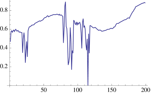
Figure 1. Linearly interpolated samples from a row of the $200\times 200$ gray scale image (Example/ocelot.jpg) in the Mathematica TestImage library.

We next consider the knot sequence on $[1,199]$ given by $\mathbf{a}:=(1,4,7,\dots,196,199)$. For each knot $a\in\mathbf{a}$ with $1\leq a<199$, let $\theta_{(\mathbf{a},a)}=1/2$. Note that for $1\leq a<196$, $\Phi_{(\mathbf{a},a)}$ consists of three orthogonal functions, and $\Phi_{(\mathbf{a},196)}$ consists of four orthogonal functions. It follows that $\dim S(\Phi_{(\mathbf{a},\cdot)})=199$. It is easy to check that there is a unique function $f\in S(\Phi_{(\mathbf{a},\cdot)})$ that interpolates the data, i.e. $f(i)=d_{i}$ for $1\leq i\leq 199$.

We now show the results of applying the greedy algorithm to the function $f$. Note that $\mathbf{a}$ has 65 interior knots. Thus in step $(1)$, we let $N=65$ and $\mathbf{a}^{65}:=\mathbf{a}$. For $1\leq i\leq 65$,

$$\|f-P_{S(\Phi_{(\mathbf{a^{i}},\cdot)})}f\|^{2}$$

represents the square of the error obtained by approximating $f$ with $P_{S(\Phi_{(\mathbf{a^{i}},\cdot)})}f$. This function of $i$ is plotted in Figure 2.

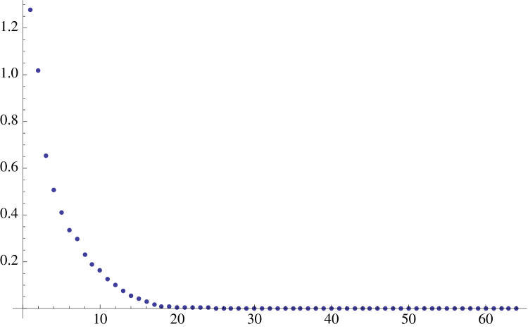
Figure 2. Error Data

For example, if $i=20$ the value of the square of the error is $0.00491487$. $\mathbf{a}^{20}$ is a knot sequence with 20 interior knots, and is the result of using the greedy algorithm to drop 45 knots, one at a time, from the original knot sequence $\mathbf{a}$ which has 65 interior knots. In Figure 3 we see the plot of $P_{S(\Phi_{(\mathbf{a^{20}},\cdot)})}f$, the plot of the original data set, and the knots in $\mathbf{a^{20}}$ on the horizontal axis.

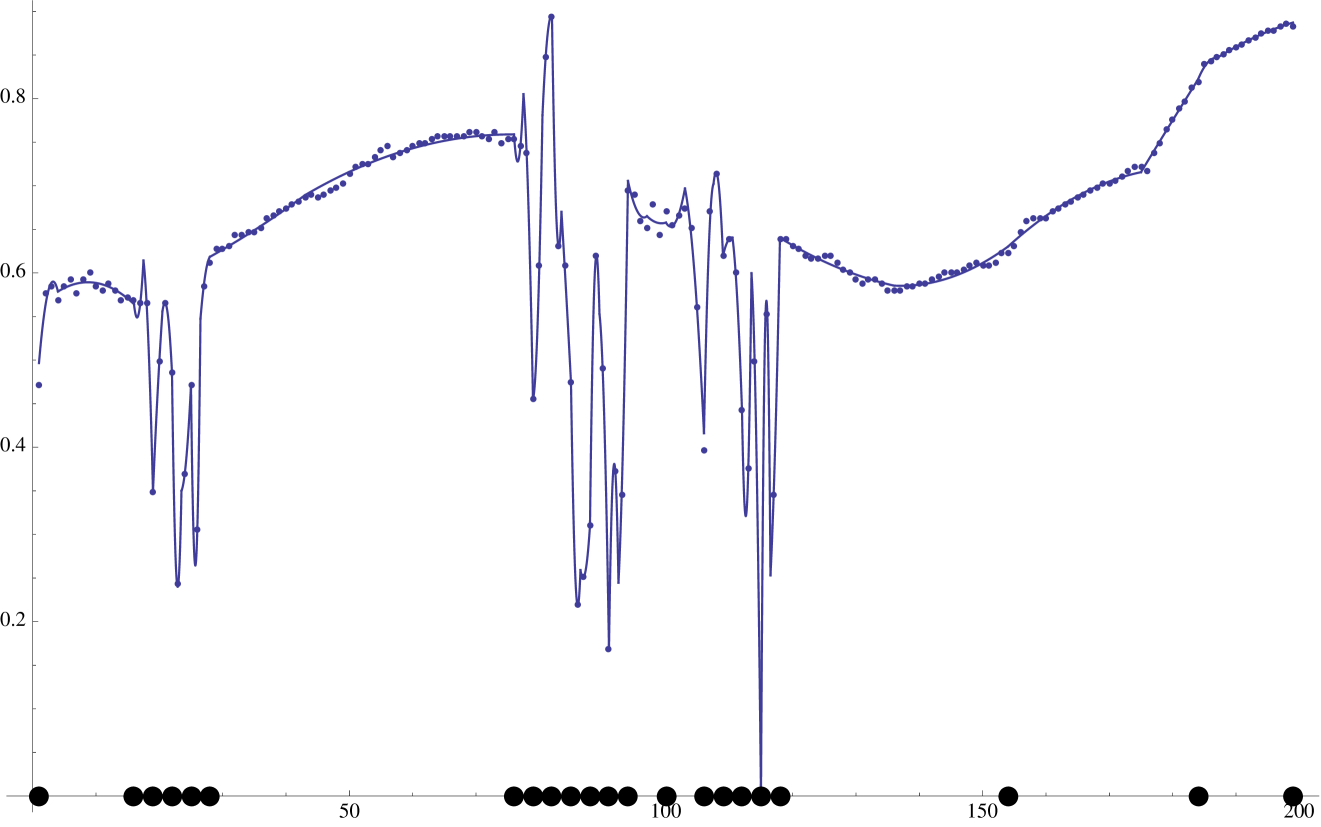
Figure 3. Continuous plot of projection with original data points and knots of $\mathbf{a^{20}}$ on the horizontal axis.

3.3. Arbitrary polynomial reproduction: Wavelet construction

For a knot sequence $\mathbf{a}$ and $n=1,2,\ldots$, let $V^{0}:=S(\Omega_{\mathbf{a}}^{n})$ and $V^{1}:=S(\Omega_{\mathbf{a}}^{n+3})$ where $\Omega_{\mathbf{a}}^{n}$ is given in Section 1.3. By Theorem 7 there is a basis $\Psi_{\mathbf{a}}^{n}$ centered on $\mathbf{a}$ such that $V^{1}=V^{0}\oplus W$ where $W=S(\Psi_{\mathbf{a}}^{n})$. We next use the algorithm from section 2.2 to construct such a $\Psi_{\mathbf{a}}^{n}$.

Recall that

$$r^{n}=(I-P_{\{\tilde{\phi}^{2},\ldots,\tilde{\phi}^{n},z^{n}\}})r=(I-P_{\{z^{n}\}})r_{n}$$

and

$$l^{n}=(I-P_{\{\tilde{\phi}^{2},\ldots,\tilde{\phi}^{n},z^{n}\}})l=(I-P_{\{z^{n}\}})l_{n}.$$

For $n=1,2,\ldots,$ let

$$\Lambda^{n}:=\text{span}\{\tilde{\phi}^{2},\ldots,\tilde{\phi}^{n},z^{n}\}.$$

Note that $\Lambda^{1}=\text{span}\{z^{1}\}$. From the definitions of $\tilde{\phi}^{n}$ and $z^{n}$ it follows that

$$\Lambda^{n+3}=\Lambda^{n}\oplus\text{span}\{\tilde{\phi}^{n+2},z^{n}_{\perp},z^{n+3}\}=\Lambda^{n}\oplus\Delta^{n},$$

where

$$z^{n}_{\perp}=\frac{\tilde{\phi}^{n+1}}{||\tilde{\phi}^{n+1}||^{2}}-\alpha_{n}\frac{\tilde{\phi}^{n+3}}{||\tilde{\phi}^{n+3}||^{2}}$$

and

$$\Delta^{n}:=\text{span}\{\tilde{\phi}^{n+2},z^{n}_{\perp},z^{n+3}\}.$$

Clearly, $z^{n}_{\perp}$ and $z^{n}$ are orthogonal and span the same space as $\tilde{\phi}^{n+1}$ and $\tilde{\phi}^{n+3}$.

Now

$$\bar{V}_{a}^{0}=\text{span }\bar{\Omega}^{n}_{a}=\text{span}\{\bar{\omega}^{n}_{a}\}$$

where $\bar{\omega}^{n}_{a}=r^{n}\circ\sigma_{a_{-}}+l^{n}\circ\sigma_{a}$. Similarly

$$\bar{V}_{a}^{1}=\text{span }\bar{\Omega}^{n+3}_{a}=\text{span}\{\bar{\omega}^{n+3}_{a}\}$$

where $\bar{\omega}^{n+3}_{a}=r^{n+3}\circ\sigma_{a_{-}}+l^{n+3}n\circ\sigma_{a}$. It follows that $\bar{k}_{a}^{0}=\bar{k}_{a}^{1}=1$ for every $a$. Furthermore tt is easy to see that for every $a$, $Y_{a}=Y_{a}^{-}=Y_{a}^{+}=\{0\}$, and so $m_{a}=m_{a}^{-}=m_{a}^{+}=0$. Lemmas 14 and 16 imply that $\dim\hat{W}_{a}^{n}=\dim\tilde{W}_{a}^{n}=1$. The superscript denotes the dependence on $n$ in the construction. From the definitions of $r^{n}$ and $l^{n}$, and the symmetries of the polynomials $\tilde{\phi}^{n}$, it can be shown that $l^{n}$ is the reflection of $r^{n}$ with respect to the line $x=1/2$. From this we can see that

$$\langle\bar{\omega}^{n}_{a},\bar{\omega}^{n}_{a}\rangle =(a_{+}-a_{-})\langle r^{n},r^{n}\rangle$$

$$\langle\bar{\omega}^{n}_{a},\bar{\omega}^{n+3}_{a}\rangle =(a_{+}-a_{-})\langle r^{n},r^{n+3}\rangle$$

Since $\Lambda^{n+3}=\Lambda^{n}\oplus\Delta^{n}$ and $r^{n}=r-P_{\Lambda^{n}}r$, we get

(45) $$r^{n}-r^{n+3}=P_{\Delta^{n}}r.$$

Now, $r^{n+3}\perp\Delta^{n}$. From this it follows that

$$\langle r^{n},r^{n+3}\rangle=\langle r^{n+3},r^{n+3}\rangle.$$

We now begin the construction of the wavelets. Since $\hat{W}_{a}^{n}$ is one dimensional equation (38) shows it is spanned by the single function $\hat{w}_{a}^{n}:=(I-P_{\bar{w}_{a}^{n}})\bar{\omega}^{n+3}_{a}$ which is,

$$\hat{w}_{a}^{n}=(r^{n+3}-\frac{\langle r^{n+3},r^{n+3}\rangle}{\langle r^{n},r^{n}\rangle}r^{n})\circ\sigma_{a_{-}}+(l^{n+3}-\frac{\langle r^{n+3},r^{n+3}\rangle}{\langle r^{n},r^{n}\rangle}l^{n})\circ\sigma_{a}.$$

Since $T_{a}^{n}=(P_{\breve{V}_{a_{-}}^{1}}+P_{\breve{V}_{a}^{1}})\bar{V}_{a}^{0}$ it to is one dimensional and by Lemma 13 it follows that $T_{a}^{-}=T_{a}^{+}=\{0\}$, and so $U_{a}^{n}=T_{a}^{n}$ hence $S_{a}^{n}$ is spanned by the single function

$$s_{a}^{n}=-(r^{n}-r^{n+3})\circ\sigma_{a_{-}}+(l^{n}-l^{n+3})\circ\sigma_{a}.$$

Equation (39) shows that $\tilde{W}_{a}^{n}$ is spanned by $(I-P_{\bar{V}_{a}^{0}\oplus\hat{W}_{a}^{n}})s_{a}^{n}$. A straightforward computation shows that this function is a scalar multiple of

$$\tilde{w}_{a}^{n}:=(r^{n}-r^{n+3})\circ\sigma_{a_{-}}-c_{a}(l^{n}-l^{n+3})\circ\sigma_{a}.$$

where

$$c_{a}=\frac{a-a_{-}}{a_{+}-a}.$$

We next construct the short wavelets. Since $\breve{k}_{a}^{0}=n$, $\breve{k}_{a}^{1}=n+3$ and from above $\bar{k}^{0}_{a}=\bar{k}^{1}_{a}=1$ it follows from Theorem 11 that $\dim\breve{W}_{a}^{n}=1$. Also from the formula for $T_{a}^{n}$ above we find

$$A_{a}^{-} =\text{ span }\{(r^{n}-r^{n+3})\circ\sigma_{a_{-}}\}$$

$$A_{a}^{+} =\text{ span }\{(l^{n}-l^{n+3})\circ\sigma_{a}\}$$

With the above results, using equation (40) and another straightforward computation we see that $\breve{W}_{a}^{n}$ is spanned by

$$\breve{w}_{a}^{n}:=\langle z^{n+3},r\rangle\tilde{\phi}^{n+2}\circ\sigma_{a}-\langle\tilde{\phi}^{n+2},r\rangle z^{n+3}\circ\sigma_{a}.$$

In summary the wavelets constructed are,

(46) $$\hat{w}_{a}^{n} =(r^{n+3}-\frac{\langle r^{n+3},r^{n+3}\rangle}{\langle r^{n},r^{n}\rangle}r^{n})\circ\sigma_{a_{-}}+(l^{n+3}-\frac{\langle r^{n+3},r^{n+3}\rangle}{\langle r^{n},r^{n}\rangle}l^{n})\circ\sigma_{a}$$

$$\tilde{w}_{a}^{n} =(r^{n}-r^{n+3})\circ\sigma_{a_{-}}-c_{a}(l^{n}-l^{n+3})\circ\sigma_{a}$$

$$\breve{w}_{a}^{n} =\langle z^{n+3},r\rangle\tilde{\phi}^{n+2}\circ\sigma_{a}-\langle\tilde{\phi}^{n+2},r\rangle z^{n+3}\circ\sigma_{a}.$$

4. $\tau$-Wavelets

4.1. Nested Knot Sequences Determined by $\tau$

Let $\tau$ denote the ”golden ratio” $\frac{1}{2}(1+\sqrt{5})$ which satisfies the quadratic relation $\tau^{2}=1+\tau$. A non-negative number $x$ is a $\tau$-rational number if it can be represented in the form $x=\sum\limits_{k=m}^{n}\varepsilon_{k}\tau^{k}$ where $m\leq n$ are integers and each $\varepsilon_{k}\in\{0,1\}$. Furthermore, $x$ is a $\tau$-integer if it has such a representation with $m=0$. By the above quadratic relation, this representation is unique if one further requires that $\varepsilon_{k}\varepsilon_{k+1}=0$ whenever $m\leq k\leq n-1$. For example, the first few non-negative $\tau$-integers are $0,1,\tau,\tau^{2},\tau^{2}+1,\tau^{3},\ldots$. We denote the set of non-negative $\tau$-integers by $\mathbf{Z}_{\tau}^{+}$. The unique representation of positive $\tau$-integers implies that $\mathbf{Z}_{\tau}^{+}\setminus\{0\}$ can be partitioned into $\tau\mathbf{Z}_{\tau}^{+}\setminus\{0\}$ and $1+\tau^{2}\mathbf{Z}_{\tau}^{+}$. Further, $\tau\mathbf{Z}_{\tau}^{+}\setminus\{0\}$ can be partitioned into $\tau+\tau^{2}\mathbf{Z}_{\tau}^{+}$ and $\tau^{2}+\tau^{3}\mathbf{Z}_{\tau}^{+}$. Also, the difference between consecutive $\tau$-integers is either $1$ or $\frac{1}{\tau}$. More specifically, considering $\mathbf{Z}_{\tau}^{+}$ as a knot sequence $\mathbf{a}$, if $a\in 1+\tau^{2}\mathbf{Z}_{\tau}^{+}$, then $a-a_{-}=1$ and $a_{+}-a=\frac{1}{\tau}$; while if $a\in\tau+\tau^{2}\mathbf{Z}_{\tau}^{+}$, then $a-a_{-}=\frac{1}{\tau}$ and $a_{+}-a=1$; and finally if $a\in\tau^{2}+\tau^{3}\mathbf{Z}_{\tau}^{+}$, then $a-a_{-}=1$ and $a_{+}-a=1$. Letting $L$ denote the “long” difference of $1$ and letting $S$ denote the “short” difference of $\frac{1}{\tau}$, we denote a non-zero $a\in\mathbf{a}$ as $LS$, respectively $SL,LL$, if $a\in 1+\tau^{2}\mathbf{Z}_{\tau}^{+}$, respectively $a\in\tau+\tau^{2}\mathbf{Z}_{\tau}^{+}$, $a\in\tau^{2}+\tau^{3}\mathbf{Z}_{\tau}^{+}$. (Note: The sequence of successive differences of elements of $\mathbf{Z}_{\tau}^{+}$ forms an infinite word,

$$f=LSLLSLSLLSLLSLSLLSLSL\ldots\text{,}$$

with alphabet $\{L,S\}$ which is invariant under the substitution $L\mapsto LS$, $S\mapsto L$. $f$ is called the Fibonacci word; see [24].)

For $k\in\mathbf{Z}$, let $\mathbf{a}^{k}$ denote the knot sequence $(\frac{1}{\tau})^{k}\mathbf{Z}_{\tau}^{+}$. The above unique representation of $\tau$-integers shows that $\mathbf{a}^{k}\subset\mathbf{a}^{k+1}$ for $k\in\mathbf{Z}$. Also, $\bigcup_{k\in\mathbf{Z}}\mathbf{a}^{k}$ is the set of non-negative $\tau$-rational numbers which can be shown to be dense in $\mathbf{R}^{+}$. For an integer $k$ and $a\in\mathbf{a}^{k}$, let $a_{-}^{k}$ (resp. $a_{+}^{k}$) denote the predecessor (resp. successor) of $a$ relative to $\mathbf{a}^{k}$. At level $k$, each interval $[a,a_{+}^{k}]$ has length either $\frac{1}{\tau^{k}}$ or $\frac{1}{\tau^{k+1}}$. Such an interval will be called long at level $k$ if it has length $\frac{1}{\tau^{k}}$ and short at level $k$ if it has length $\frac{1}{\tau^{k+1}}$. The refinement from level $k$ to level $k+1$ proceeds as follows. Each long interval at level $k$ is split into two subintervals $[a,a_{+}^{k+1}]$ and $[a_{+}^{k+1},a_{+}^{k}]$, where

(47) $$a_{+}^{k+1}=(1-\frac{1}{\tau})a+\frac{1}{\tau}a_{+}^{k}.$$

It follows that the left subinterval $[a,a_{+}^{k+1}]$ is long at level $k+1$, and the right subinterval $[a_{+}^{k+1},a_{+}^{k}]$ is short at level $k+1$. Each short interval at level $k$ is not subdivided and becomes long at level $k+1$; i.e. if $a_{+}^{k}-a=\frac{1}{\tau^{k+1}}$ then $a_{+}^{k}=a_{+}^{k+1}$.

4.2. $\tau$-Wavelets of Haar

We now show that the $\tau$-wavelets of Haar, constructed in [19], can be considered as a special case of the general wavelet construction outlined in Section 2.2. Let $\phi_{1}:=\chi_{[0,1]}$, $\phi_{2}:=\tau^{\frac{1}{2}}\chi_{[0,\frac{1}{\tau}]}$, and $\Phi=\{\phi_{1}(\cdot-b)\mid b\in\tau\mathbf{Z}_{\tau}^{+}\}\cup\{\phi_{2}(\cdot-c)\mid c\in 1+\tau^{2}\mathbf{Z}_{\tau}^{+}\}$. Then $\Phi$ is an orthonormal basis centered on $\mathbf{Z}_{\tau}^{+}$ that is generated by appropriate $\tau$-integer translations of $\phi_{1}$ and $\phi_{2}$ and $S(\Phi)$ is the space of piecewise constant functions in $L^{2}(\mathbf{R}^{+})$ with breakpoints in $\mathbf{Z}_{\tau}^{+}$. For $k\in\mathbf{Z}$, let $\Phi^{k}:=\{\tau^{\frac{k}{2}}f(\tau^{k}\cdot)\mid f\in\Phi\}$ ($=\{\tau^{\frac{k}{2}}\phi_{1}(\tau^{k}\cdot-b)\mid b\in\tau\mathbf{Z}_{\tau}^{+}\}\cup\{\tau^{\frac{k}{2}}\phi_{2}(\tau^{k}\cdot-c)\mid c\in 1+\tau^{2}\mathbf{Z}_{\tau}^{+}\}$). Then $\Phi^{k}$ is an orthonormal basis centered on $\mathbf{a}^{k}$ and $S(\Phi^{k})$ is the space of piecewise constant functions in $L^{2}(\mathbf{R}^{+})$ with breakpoints in $\mathbf{a}^{k}$.

Since $\mathbf{a}^{k}\subset\mathbf{a}^{k+1}$ for $k\in\mathbf{Z}$, it follows that $S(\Phi^{k})\subset S(\Phi^{k+1})$ for $k\in\mathbf{Z}$. In particular, $\Phi^{0}$ and $\Phi^{1}$ are orthonormal bases centered on $\mathbf{Z}_{\tau}^{+}$ and $S(\Phi^{0})\subset S(\Phi^{1})$. Theorem 7 thus applies to this situation. We construct $\Psi$ as outlined in Section 2.2.

For $a>0\in\mathbf{Z}_{\tau}^{+}$, it is easy to see that $\bar{k}_{a}^{0}=\bar{k}_{a}^{1}=m_{a}=m_{a}^{\pm}=0$. Also, $\breve{k}_{a}^{0}=1$ for every $a\in\mathbf{Z}_{\tau}^{+}$. For $a\in\mathbf{Z}_{\tau}^{+}$, it follows from the manner in which $\mathbf{a}^{0}$ is refined to $\mathbf{a}^{1}$ that

$$\breve{k}_{a}^{1}=\begin{cases}1&\text{if }a\in 1+\tau^{2}\mathbf{Z}_{\tau}^{+}\\ 2&\text{if }a\in\tau\mathbf{Z}_{\tau}^{+}.\end{cases}$$

Thus Theorem 11 implies that $\bar{W}_{a}=\{0\}$ for $a>0\in\mathbf{Z}_{\tau}^{+}$, and

$$\dim\breve{W}_{a}=\begin{cases}0&\text{if }a\in 1+\tau^{2}\mathbf{Z}_{\tau}^{+}\\ 1&\text{if }a\in\tau\mathbf{Z}_{\tau}^{+}.\end{cases}$$

From equation (34), for $a\in\tau\mathbf{Z}_{\tau}^{+}$ we have $\breve{W}_{a}=(I-P_{\breve{V}_{a}^{0}})\breve{V}_{a}^{1}$. Also, for $a\in\tau\mathbf{Z}_{\tau}^{+}$, $\breve{V}_{a}^{0}$ is spanned by the function $\chi_{[a,a_{+}]}$ and $\breve{V}_{a}^{1}$ is spanned by the functions $\chi_{[a,a+\frac{1}{\tau}]}$ and $\chi_{[a+\frac{1}{\tau},a_{+}]}$. An easy computation shows that an orthonormal basis for $\breve{W}_{a}$ consists of the single function $\tau^{-\frac{1}{2}}\chi_{[a,a+\frac{1}{\tau}]}-\tau^{\frac{1}{2}}\chi_{[a+\frac{1}{\tau},a_{+}]}.$

With

$$\psi:=\tau^{-\frac{1}{2}}\chi_{[0,\frac{1}{\tau}]}-\tau^{\frac{1}{2}}\chi_{[\frac{1}{\tau},1]},$$

it follows that $W=S(\Psi)$ where $\Psi:=\{\psi(\cdot-b)\mid b\in\tau\mathbf{Z}_{\tau}^{+}\}$. Note that $\Psi$ is an orthonormal basis centered on $\mathbf{Z}_{\tau}^{+}$, obtained by appropriate $\tau$-integer translations of $\psi$. Letting $\Psi^{k}:=\{\tau^{\frac{k}{2}}\psi(\tau^{k}\cdot-b)\mid b\in\tau\mathbf{Z}_{\tau}^{+}\}$, for $k\in\mathbf{Z}$, it is easy to check that $\Psi^{k}$ is a basis centered on $\mathbf{a}^{k}$ and that $S(\Phi^{k})\oplus S(\Psi^{k})=S(\Phi^{k+1})$. Since $\bigcap\limits_{k\in\mathbf{Z}}S(\Phi^{k})=\{0\}$ and $\bigcup\limits_{k\in\mathbf{Z}}S(\Phi^{k})$ is dense in $L^{2}(\mathbf{R}^{+})$, it follows that $L^{2}(\mathbf{R}^{+})=\bigoplus\limits_{k\in\mathbf{Z}}S(\Psi^{k})$, i.e. $\{\tau^{\frac{k}{2}}\psi(\tau^{k}\cdot-b)\mid k\in\mathbf{Z,}b\in\tau\mathbf{Z}_{\tau}^{+}\}$ is an orthonormal basis of $L^{2}(\mathbf{R}^{+})$. These functions are called the $\tau$-wavelets of Haar in [19].

4.3. Continuous, Piecewise Quadratic $\tau$-Wavelets

Let

(48) $$\Phi^{k}:=\Omega_{\mathbf{a}^{k},\boldsymbol{\theta}},\qquad k\in{\bf Z}$$

denote the continuous, piecewise quadratic, orthonormal basis centered on $\mathbf{a}^{k}$ as described in Section 1.4 with constant parameter sequence $\boldsymbol{\theta}=\left(\theta_{a}\right)_{a\in\mathbf{a}^{k}}$ where $\theta_{a}=1/\tau$ for $a\in\mathbf{a}^{k}$ (here we assume that the components of $\Phi^{k}$ have been normalized). It follows from (47) that $(\mathbf{a}^{k},\boldsymbol{\theta})$ satisfy the hypotheses of Proposition 6. Since, as previously discussed $\bigcup_{k}\mathbf{a}^{k}$ is dense in $J={\bf R}_{+}$ and since $\boldsymbol{\alpha}=\bigcap_{k}\mathbf{a}^{k}\cup\mathbf{b}(\mathbf{a}^{k},\boldsymbol{\theta}^{k})=\{0\}$, Proposition 6 implies that the spaces $V^{k}:=S(\Phi^{k})$ form a multiresolution analysis of $L^{2}({\bf R}_{+})$, that is,

1. $V^{k}\subset V^{k+1},\qquad(k\in{\bf Z})$,

2. $\bigcup_{k}V^{k}$ is dense in $L^{2}({\bf R}_{+})$,

3. $\bigcap_{k}V^{k}=\{0\}$.

As in the $\tau$-wavelets of Haar construction, the basis $\Phi:=\Phi^{0}$ centered on the knot sequence $\mathbf{a}^{0}=\mathbf{Z}_{\tau}^{+}$ for $V_{0}$ can also be generated by the $\tau$-integer translations of a small number of functions in $\Phi$. Suppose $a$ and $a^{\prime}$ in $\mathbf{Z}_{\tau}^{+}\setminus\{0\}$ have the same classification (say $LS$), then from the construction of $\Phi$ it follows that $\Phi_{a}$ is a translate of $\Phi_{a^{\prime}}$. (Note: Here $\Phi_{a}$ stands for the more cumbersome, yet precise, $\Phi_{a,\mathbf{a}^{0}}^{0}$; see section 1.) Specifically, we have, for $b\in\mathbf{Z}_{\tau}^{+}$,

$$\Phi_{1+\tau^{2}b}(\cdot) = \Phi_{1}(\cdot-\tau^{2}b),$$

(49) $$\Phi_{\tau+\tau^{2}b}(\cdot) = \Phi_{\tau}(\cdot-\tau^{2}b),$$

$$\Phi_{\tau^{2}+\tau^{3}b}(\cdot) = \Phi_{\tau^{2}}(\cdot-\tau^{3}b).$$

Thus every function in $\Phi$, with the exception of those in $\Phi_{0}$, is a $\tau$-integer translate of a function from $\Phi_{1},$ $\Phi_{\tau},$ or $\Phi_{\tau^{2}}$. For any positive $a\in\mathbf{Z}_{\tau}^{+}$, let

$$\beta(a):=\begin{cases}1&\text{if $a\in 1+\tau^{2}\mathbf{Z}^{+}_{\tau}$,}\\ \tau&\text{if $a\in\tau+\tau^{2}\mathbf{Z}^{+}_{\tau}$,}\\ \tau^{2}&\text{if $a\in\tau^{2}+\tau^{3}\mathbf{Z}^{+}_{\tau},$}\end{cases}$$

and $\mu(a):=a-\beta(a)$. Then $a=\beta(a)+\mu(a)$ where $\beta(a)\in\{1,\tau,\tau^{2}\}$ and $\mu(a)\in\tau^{2}\mathbf{Z}_{\tau}^{+}$ if $\beta(a)=1$ or $\tau$ and $\mu(a)\in\tau^{3}\mathbf{Z}_{\tau}^{+}$ if $\beta(a)=\tau^{2}$. Thus, we can write (49) in the more compact form

(50) $$\Phi_{a}=\Phi_{\beta(a)}(\cdot-\mu(a))\qquad(a\in\mathbf{Z}_{\tau}^{+}\setminus\{0\}).$$

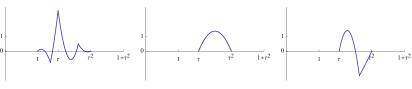
Figure 4. $\Phi_{\tau}$.

For $k\in\mathbf{Z}$ and $a\in\mathbf{Z}_{\tau}^{+}$, let

$$\Phi_{k,a}=\tau^{k/2}\Phi_{a}(\tau^{k}\cdot).$$

We remark that with this definition, $\Phi_{k,a}=\Phi^{k}_{a/\tau^{k},\mathbf{a}^{k}}$, and we apologize for the confusing notation. Note that $V^{0}\subset V^{1}$ and both $\Phi^{0}$ and $\Phi^{1}$ can be regarded as orthonormal bases centered on the knot sequence $\mathbf{a}^{0}=\mathbf{Z}_{\tau}^{+}$. For $a\in\mathbf{a}^{0}$, $\Phi_{a}^{1}$ will denote the more precise $\Phi_{a,\mathbf{a}^{0}}^{1}$. It follows that we have the following ‘polyphase’ like representation:

$$\Phi_{0}^{1}=\left[\begin{matrix}\Phi_{1,0}\\ \Phi_{1,1}\end{matrix}\right],\Phi_{1}^{1}=\Phi_{1,\tau},\Phi_{\tau}^{1}=\left[\begin{matrix}\Phi_{1,\tau^{2}}\\ \Phi_{1,1+\tau^{2}}\end{matrix}\right],~{}\text{and}~{}\Phi_{\tau^{2}}^{1}=\left[\begin{matrix}\Phi_{1,\tau^{3}}\\ \Phi_{1,1+\tau^{3}}\end{matrix}\right].$$

Figure 4 shows the three functions in $\Phi_{\tau}$ and Figure 5 shows the six functions in $\Phi_{\tau}^{1}$.

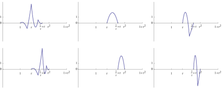
Figure 5. $\Phi_{\tau}^{1}$.

For $a\in\mathbf{Z}_{\tau}^{+}$ and $a>\tau^{2}$,

$$\Phi_{a}^{1}=\Phi_{\beta(a)}^{1}(\cdot-\mu(a)).$$

The coefficient matrices from section 2.3 can now be computed. For $a\in\mathbf{Z}_{\tau}^{+}$ and $a^{\prime}\in\{a_{-},a\}$, $c_{aa^{\prime}}=\langle\Phi_{a},\Phi_{a^{\prime}}^{1}\rangle$. In particular we have

$$\Phi_{0}=c_{00}\Phi_{0}^{1},~{}\text{and}~{}\Phi_{a}=c_{aa_{-}}\Phi_{a_{-}}^{1}+c_{aa}\Phi_{a}^{1},~{}\text{for}~{}a>0.$$

For any $k\in\mathbf{Z}$, $V^{k}\subset V^{k+1}$ and both $\Phi^{k}$ and $\Phi^{k+1}$ can be regarded as orthonormal bases centered on the knot sequence $\mathbf{a}^{k}$. For $a\in\mathbf{Z}_{\tau}^{+}$ it follows that $\Phi_{a/\tau^{k},\mathbf{a}^{k}}^{k+1}=\tau^{k/2}\Phi_{a}^{1}(\tau^{k}\cdot)$. We have, for $b\in\mathbf{a}^{k}$,

$$\Phi_{0,\mathbf{a}^{k}}^{k}=c_{00}\Phi_{0,\mathbf{a}^{k}}^{k+1},~{}\text{and}~{}\Phi_{b,\mathbf{a}^{k}}^{k}=c_{(\tau^{k}b)(\tau^{k}b)_{-}}\Phi_{b_{-},\mathbf{a}^{k}}^{k+1}+c_{(\tau^{k}b)(\tau^{k}b)}\Phi_{b,\mathbf{a}^{k}}^{k+1}~{}\text{for}~{}b>0.$$

(Note: In the second equation above there are two occurrences of the minus subscript. The first denotes the predecessor of $\tau^{k}b$ in the knot sequence $\mathbf{a}^{0}$. The second denotes the predecessor of $b$ in the knot sequence $\mathbf{a}^{k}$. See section 1.)

Recall that

$$\Phi_{0}^{1}=\left[\begin{matrix}\Phi_{1,0}\\ \Phi_{1,1}\end{matrix}\right].$$

Thus

$$c_{00}=\langle\Phi_{0},\Phi_{0}^{1}\rangle=\left[\begin{matrix}\langle\Phi_{0},\Phi_{1,0}\rangle&\langle\Phi_{0},\Phi_{1,1}\rangle\end{matrix}\right].$$

Letting,

$$C_{a,a^{\prime}}:=\langle\Phi_{a},\Phi_{1,a^{\prime}}\rangle,$$

for $a,a^{\prime}\in\mathbf{Z}^{+}_{\tau}$, we now have

$$c_{00}=\left[\begin{matrix}C_{0,0}&C_{0,1}\end{matrix}\right]~{}\text{and}~{}c_{10}=\left[\begin{matrix}C_{1,0}&C_{1,1}\end{matrix}\right].$$

and, similarly, $c_{11}=C_{1,\tau}$, $c_{\tau 1}=0$,

$$c_{\tau\tau}=\left[\begin{matrix}C_{\tau,\tau^{2}}&C_{\tau,1+\tau^{2}}\end{matrix}\right],c_{\tau^{2}\tau}=\left[\begin{matrix}C_{\tau^{2},\tau^{2}}&C_{\tau^{2},1+\tau^{2}}\end{matrix}\right],$$

and

$$c_{\tau^{2}\tau^{2}}=\left[\begin{matrix}C_{\tau^{2},\tau^{3}}&C_{\tau^{2},1+\tau^{3}}\end{matrix}\right].$$

For $a>\tau^{2}$, $c_{aa}=c_{\beta(a)\beta(a)}$ and $c_{aa_{-}}=c_{\beta(a)\beta(a)_{-}}$.

In Table 1 we provide (with the aid of Mathematica™) the matrices $C_{a,a^{\prime}}$ defined above. Here we assume that $\Phi_{a}$ is ordered as follows: of the three components, the second and third components are the “$q$” and “$z$” components from $\breve{\Phi}_{a}$, respectively, while the first component is the component of $\Phi_{a}$ that does not vanish at $a$.

Table 1. Scaling Coefficients for $\Phi$

$$C_{0,0} =\left(\begin{array}[]{lll}\sqrt{-\frac{1}{2}+\frac{\sqrt{5}}{2}}&-\frac{1}{2\sqrt{16491+7375\sqrt{5}}}&\frac{121}{2\sqrt{5485+2441\sqrt{5}}}\\ 0&\frac{1}{4}\sqrt{-818+370\sqrt{5}}&-\sqrt{\frac{55}{2\left(405+181\sqrt{5}\right)}}\\ 0&\frac{251}{\sqrt{76350+33982\sqrt{5}}}&\frac{59}{\sqrt{30410+13610\sqrt{5}}}\end{array}\right)$$

$$C_{0,1} =\left(\begin{array}[]{lll}19\sqrt{\frac{2}{9765+4387\sqrt{5}}}&\frac{1}{2}\sqrt{\frac{11}{767+343\sqrt{5}}}&\frac{19}{2}\sqrt{\frac{5}{25615+11463\sqrt{5}}}\\ \sqrt{\frac{2}{11}\left(-35+16\sqrt{5}\right)}&\frac{1}{4}\left(13-5\sqrt{5}\right)&\frac{5}{\sqrt{370+166\sqrt{5}}}\\ -\frac{1}{11}\sqrt{\frac{5922}{5}-\frac{2584}{\sqrt{5}}}&-\sqrt{-\frac{283}{8}+\frac{637}{8\sqrt{5}}}&\frac{1}{44}\left(-129+53\sqrt{5}\right)\end{array}\right)$$

$$C_{1,0} =\left(\begin{array}[]{lll}0&-\frac{1}{2}\sqrt{\frac{11}{1715+767\sqrt{5}}}&\frac{11}{\sqrt{2}\left(35+17\sqrt{5}\right)}\\ 0&0&0\\ 0&0&0\end{array}\right)$$

$$C_{1,1} =\left(\begin{array}[]{lll}-\sqrt{-\frac{2}{5}+\frac{1}{\sqrt{5}}}&\frac{1}{4}\sqrt{177-\frac{389}{\sqrt{5}}}&-\frac{1}{4}\sqrt{-89+41\sqrt{5}}\\ 0&0&0\\ 0&0&0\end{array}\right)$$

$$C_{1,\tau} =\left(\begin{array}[]{lll}3-\sqrt{5}&0&0\\ 0&1&0\\ 0&0&1\end{array}\right)$$

$$C_{\tau,\tau^{2}} =\left(\begin{array}[]{lll}\frac{1}{2}\sqrt{\frac{1}{2}\left(13-3\sqrt{5}\right)}&-\frac{1}{4}\sqrt{\frac{5}{36875+16491\sqrt{5}}}&\frac{121}{4\sqrt{2441+1097\sqrt{5}}}\\ 0&\sqrt{-\frac{409}{8}+\frac{185\sqrt{5}}{8}}&-\sqrt{\frac{55}{2\left(405+181\sqrt{5}\right)}}\\ 0&\frac{251}{\sqrt{76350+33982\sqrt{5}}}&\frac{59}{\sqrt{30410+13610\sqrt{5}}}\end{array}\right)$$

$$C_{\tau,\tau^{2}+1} =\left(\begin{array}[]{lll}\frac{1}{44}\left(-63+31\sqrt{5}\right)&\frac{1}{4}\sqrt{\frac{55}{1715+767\sqrt{5}}}&\frac{19}{4}\sqrt{\frac{5}{11463+5123\sqrt{5}}}\\ \sqrt{\frac{2}{11}\left(-35+16\sqrt{5}\right)}&\frac{1}{4}\left(13-5\sqrt{5}\right)&\frac{5}{\sqrt{370+166\sqrt{5}}}\\ -\frac{1}{11}\sqrt{\frac{5922}{5}-\frac{2584}{\sqrt{5}}}&-\sqrt{-\frac{283}{8}+\frac{637}{8\sqrt{5}}}&\frac{1}{44}\left(-129+53\sqrt{5}\right)\end{array}\right)$$

$$C_{\tau^{2},\tau^{2}} =\ \left(\begin{array}[]{lll}0&-\frac{1}{2}\sqrt{\frac{11}{2\left(1030+461\sqrt{5}\right)}}&\frac{1}{2}\sqrt{\frac{1}{310}\left(166-69\sqrt{5}\right)}\\ 0&0&0\\ 0&0&0\end{array}\right)$$

$$C_{\tau^{2},\tau^{2}+1} =\left(\begin{array}[]{lll}-\sqrt{\frac{1}{310}+\frac{\sqrt{5}}{62}}&\frac{1}{2}\sqrt{\frac{1}{310}\left(625-192\sqrt{5}\right)}&-\sqrt{-\frac{37}{248}+\frac{4\sqrt{5}}{31}}\\ 0&0&0\\ 0&0&0\end{array}\right)$$

$$C_{\tau^{2},\tau^{3}} =\left(\begin{array}[]{lll}2\sqrt{\frac{1}{31}\left(6-\sqrt{5}\right)}&-\frac{1}{2}\sqrt{\frac{5}{2\left(93850+41971\sqrt{5}\right)}}&\frac{121}{2\sqrt{12492+5554\sqrt{5}}}\\ 0&\sqrt{-\frac{409}{8}+\frac{185\sqrt{5}}{8}}&-\sqrt{\frac{55}{2\left(405+181\sqrt{5}\right)}}\\ 0&\frac{251}{\sqrt{76350+33982\sqrt{5}}}&\frac{59}{\sqrt{30410+13610\sqrt{5}}}\end{array}\right)$$

$$C_{\tau^{2},\tau^{3}+1} =\left(\begin{array}[]{lll}19\sqrt{\frac{2}{22219+9991\sqrt{5}}}&\frac{1}{2}\sqrt{\frac{55}{2\left(4365+1952\sqrt{5}\right)}}&\frac{19}{2}\sqrt{\frac{5}{58306+26096\sqrt{5}}}\\ \sqrt{\frac{2}{11}\left(-35+16\sqrt{5}\right)}&\frac{1}{4}\left(13-5\sqrt{5}\right)&\frac{5}{\sqrt{370+166\sqrt{5}}}\\ -\frac{1}{11}\sqrt{\frac{5922}{5}-\frac{2584}{\sqrt{5}}}&-\sqrt{-\frac{283}{8}+\frac{637}{8\sqrt{5}}}&\frac{1}{44}\left(-129+53\sqrt{5}\right)\end{array}\right)$$

We now construct an orthogonal wavelet basis $\Psi$, centered on $\mathbf{a}^{0}$, for the continuous, piecewise quadratic scaling functions $\Phi$ such that

$$S(\Phi^{0})\oplus S(\Psi)=S(\Phi^{1})$$

using the method from section 2.2. As mentioned above this provides an example where the spaces $T^{\pm}_{a}$ contain non-zero functions.

Following Section 2.2, we determine the dimensions $\bar{k}_{a}^{\epsilon},m_{a},\text{and}~{}m_{a}^{\pm}$. If $a>0$ then $\bar{k}_{a}^{0}=\bar{k}_{a}^{1}=1$ and $m_{a}=0$. Also, for $a>0$,

(51) $$m_{a}^{+}=\begin{cases}1&\text{if}~{}a\in 1+\tau^{2}{\bf Z}_{\tau}^{+}\\ 0&\text{otherwise}\end{cases}$$

and

(52) $$m_{a}^{-}=\begin{cases}1&\text{if}~{}a\in\tau+\tau^{2}{\bf Z}_{\tau}^{+}\\ 0&\text{otherwise}.\end{cases}$$

From Theorem 11 we get

$$\dim\bar{W}_{a}=\begin{cases}1&\text{if either}~{}a\in 1+\tau^{2}{\bf Z}_{\tau}^{+}~{}\text{or}~{}a\in\tau+\tau^{2}{\bf Z}_{\tau}^{+}\\ 2&\text{if}~{}a\in\tau^{2}+\tau^{3}{\bf Z}_{\tau}^{+}.\end{cases}$$

It follows that for $a\in 1+\tau^{2}{\bf Z}_{\tau}^{+}~{}\text{or}~{}a\in\tau+\tau^{2}{\bf Z}_{\tau}^{+}$ that $\bar{W}_{a}=\hat{W}_{a}$ which is spanned by a single function. For $a\in\tau^{2}+\tau^{3}{\bf Z}_{\tau}^{+}$, a basis for $\bar{W}_{a}$ consists of two functions, one forming a basis for $\hat{W}_{a}$ and the other a basis for $\tilde{W}_{a}$. In all cases, Lemma 14 implies that for $a>0$, $\dim\hat{W}_{a}=1$. To find a basis for $\hat{W}_{a}$ we begin by constructing bases for $\hat{W}_{1},\hat{W}_{\tau}$, and $\hat{W}_{\tau^{2}}$. We use the notation introduced in Section 1.4.

For $a>0$ an orthonormal basis of $\bar{V}_{a}^{0}$ consists of the single function $\bar{\phi}_{a}^{0}$ which is a suitable scalar multiple of $r^{1/\tau}\circ\sigma_{a_{-}}+l^{1/\tau}\circ\sigma_{a}.$ It follows that an orthonormal basis of $\bar{V}_{1}^{1}$ consists of a single function $\bar{\phi}_{1}^{1}$ which is a suitable scalar multiple of $\bar{\phi}_{\tau}^{0}(\tau\cdot)$. Similarly an orthonormal basis of $\bar{V}_{\tau}^{1}$ consists of a single function $\bar{\phi}_{\tau}^{1}$ which is a suitable scalar multiple of $\bar{\phi}_{\tau^{2}}^{0}(\tau\cdot)$, and an orthonormal basis of $\bar{V}_{\tau^{2}}^{1}$ consists of a single function $\bar{\phi}_{\tau^{2}}^{1}$ which is a suitable scalar multiple of $\bar{\phi}_{\tau^{3}}^{0}(\tau\cdot)$.

For $a=1,\tau,\tau^{2}$, let

$$\hat{w}_{a}:=c_{\hat{w}_{a}}(\bar{\phi}_{a}^{1}-\langle\bar{\phi}_{a}^{1},\bar{\phi}_{a}^{0}\rangle\bar{\phi}_{a}^{0}),$$

where $c_{\hat{w}_{a}}$ is a constant so the $\|\hat{w}_{a}\|=1$. By construction for each $a>0$

(53) $$\hat{w}_{a}=\hat{w}_{\beta(a)}\big{(}\cdot-\mu(a)\big{)}$$

forms an orthonormal basis for the one dimensional space $\hat{W}_{a}$. Figure 6 shows the graphs of $\hat{w}_{1},\hat{w}_{\tau}$, and $\hat{w}_{\tau^{2}}$.

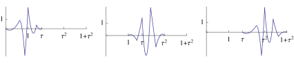
Figure 6. $\hat{w}_{a}$ for $a=1,\tau,\tau^{2}$

Next we construct a basis for $\tilde{W}_{\tau^{2}}$. We begin by constructing the spaces defined in Section 2.1. A basis for $T_{\tau^{2}}$ consists of the single function

$$t_{\tau^{2}}:=\bar{\phi}_{\tau^{2}}^{0}-\langle\bar{\phi}_{\tau^{2}}^{0},\bar{\phi}_{\tau^{2}}^{1}\rangle\bar{\phi}_{\tau^{2}}^{1}.$$

Since $m_{\tau^{2}}=m_{\tau^{2}}^{+}=m_{\tau^{2}}^{-}=0$, by equations (51) and (52), it follows from Lemma 13 that $U_{\tau^{2}}=T_{\tau^{2}}$. Thus $S_{\tau^{2}}$ is spanned by the single function

$$s_{\tau^{2}}:=(\chi_{[\tau^{2},1+\tau^{2}]}-\chi_{[\tau,\tau^{2}]})t_{\tau^{2}},$$

and so, by Lemma 16, an orthonormal basis of $\tilde{W}_{\tau^{2}}$ consists of the single function

$$\tilde{w}_{\tau^{2}}:=c_{\tilde{w}_{\tau^{2}}}(s_{\tau^{2}}-\langle s_{\tau^{2}},\bar{\phi}_{\tau^{2}}^{0}\rangle\bar{\phi}_{\tau^{2}}^{0}-\langle s_{\tau^{2}},\hat{w}_{\tau^{2}}\rangle\hat{w}_{\tau^{2}}),$$

where $c_{\tilde{w}_{\tau^{2}}}$ is chosen so that $\tilde{w}_{\tau^{2}}$ is of norm one. It follows that for $b\in{\bf Z}_{\tau}^{+}$, an orthonormal basis for $\tilde{W}_{\tau^{2}+b\tau^{3}}$ consists of the single function

(54) $$\tilde{w}_{\tau^{2}+b\tau^{3}}=\tilde{w}_{\tau^{2}}(\cdot-b\tau^{3}).$$

In Figure 7 we see $\tilde{w}_{\tau^{2}}$.

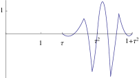
Figure 7. $\tilde{w}_{\tau^{2}}$

Completing the wavelet construction, we next determine $\breve{W}_{a}$ for $a\geq 0$. Observe that

$$\breve{k}_{a}^{0}=\begin{cases}3&\text{if}~{}a=0\\ 2&\text{if}~{}a>0\end{cases}$$

and

$$\breve{k}_{a}^{1}=\begin{cases}6&\text{if}~{}a=0\\ 2&\text{if}~{}a\in 1+\tau^{2}{\bf Z}_{\tau}^{+}\\ 5&\text{if}~{}a>0\in\tau{\bf Z}_{\tau}^{+}.\end{cases}$$

It follows from Theorem 11 and equations (51) and (52) that

$$\dim\breve{W}_{a}=\begin{cases}2&\text{if}~{}a=0\\ 0&\text{if}~{}a\in 1+\tau^{2}{\bf Z}_{\tau}^{+}\\ 1&\text{if}~{}a\in\tau{\bf Z}_{\tau}^{+}\setminus\{0\}.\end{cases}$$

We construct the spaces $\breve{W}_{a}$ using equation (34). Note that for any $a>0$, $A_{a}^{-}$ is spanned by the single function

$$f_{a}^{-}:=(\bar{\phi}_{a}^{0}-\langle\bar{\phi}_{a}^{0},\bar{\phi}_{a}^{1}\rangle\bar{\phi}_{a}^{1})\chi_{[a_{-},a]},$$

and $A_{a}^{+}$ is spanned by the single function

$$f_{a}^{+}:=(\bar{\phi}_{a}^{0}-\langle\bar{\phi}_{a}^{0},\bar{\phi}_{a}^{1}\rangle\bar{\phi}_{a}^{1})\chi_{[a,a_{+}]}.$$

We first observe that $\bar{\phi}_{1+\tau^{2}}^{0}(\tau\cdot)\in\breve{V}_{\tau}^{1}$. Also, $\breve{V}_{\tau}^{0}$ is spanned by the functions $q\circ\sigma_{\tau}$ and $z^{1/\tau}\circ\sigma_{\tau}$. Let

$$\breve{w}_{\tau}:=\breve{c}_{\tau}(I-P_{\text{ span }\{f_{\tau}^{+},q\circ\sigma_{\tau},z^{1/\tau}\circ\sigma_{\tau},f_{\tau^{2}}^{-}\}})\bar{\phi}_{1+\tau^{2}}^{0}(\tau\cdot),$$

where $\breve{c}_{\tau}$ is a normalization constant. Since dim $\breve{W}_{\tau}=1$, it follows that $\breve{w}_{\tau}$ forms an orthonormal basis for $\breve{W}_{\tau}$. Furthermore, $\breve{w}_{\tau^{2}}:=\breve{w}_{\tau}(\cdot-1)$ forms an orthonormal basis for $\breve{W}_{\tau^{2}}$.

For $b\in{\bf Z}_{\tau}^{+}$, we then define

$$\breve{w}_{\tau+\tau^{2}b} :=\breve{w}_{\tau}(\cdot-\tau^{2}b)$$

$$\breve{w}_{\tau^{2}+\tau^{3}b} :=\breve{w}_{\tau^{2}}(\cdot-\tau^{3}b).$$

It follows that for $b\in{\bf Z}_{\tau}^{+}$, $\breve{w}_{\tau+\tau^{2}b}$ (resp. $\breve{w}_{\tau^{2}+\tau^{3}b}$ ) forms an orthonormal basis for $\breve{W}_{\tau+\tau^{2}b}$ (resp. $\breve{W}_{\tau^{2}+\tau^{3}b}$). Figure 8 shows the graph of $\breve{w}_{\tau}$.

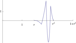
Figure 8. $\breve{w}_{\tau}$

Recall that $\breve{W}_{0}=\breve{V}_{0}^{1}\ominus(\breve{V}_{0}^{0}\oplus A_{1}^{-})$ and that $\dim\breve{W}_{0}=2$. It is easy to check that $\breve{w}_{0,1}:=\breve{w}_{\tau}(\cdot+\tau)$ is an element of $\breve{W}_{0}$. Then $\breve{w}_{0,2}$ is chosen to be the unique (up to a sign) element in $\breve{W}_{0}$ so that $\{\breve{w}_{0,1},\breve{w}_{0,2}\}$ is an orthonormal basis for $\breve{W}_{0}$. Figure 9 shows the graph of $\breve{w}_{0,2}$.

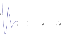
Figure 9. $\breve{w}_{0,2}$

We now have that

$$\Psi_{0}=\left[\begin{matrix}\breve{w}_{0,1}\\ \breve{w}_{0,2}\end{matrix}\right],\Psi_{1}=\left[\begin{matrix}\hat{w}_{1}\end{matrix}\right],\Psi_{\tau}=\left[\begin{matrix}\hat{w}_{\tau}\\ \breve{w}_{\tau}\end{matrix}\right],~{}\text{and}~{}\Psi_{\tau^{2}}=\left[\begin{matrix}\hat{w}_{\tau^{2}}\\ \tilde{w}_{\tau^{2}}\\ \breve{w}_{\tau^{2}}\end{matrix}\right].$$

For $a>\tau^{2}$, it follows from (50) that $\Psi_{a}=\Psi_{\beta(a)}(\cdot-\mu(a))$.

Since $S(\Phi^{k})\subset S(\Phi^{k+1})$, for $k\in\mathbf{Z}$, it follows from Theorem 7 that there exists an orthonormal basis, $\Psi^{k}$ centered on $\mathbf{a}^{k}$ so that $S(\Phi^{k+1})=S(\Phi^{k})\oplus S(\Psi^{k})$. For $k\in\mathbf{Z}$ and $a\in\mathbf{Z}_{\tau}^{+}$, let

$$\Psi_{k,a}:=\tau^{k/2}\Psi_{a}(\tau^{k}\cdot).$$

Then, for $k\in\mathbf{Z}$ and $b\in\mathbf{a}^{k}$,

$$\Psi_{b,\mathbf{a}^{k}}^{k}=\Psi_{k,\tau^{k}b}.$$

The wavelet coefficient matrices from section 2.3 can now be computed. For $a\in\mathbf{Z}_{\tau}^{+}$ and $a^{\prime}\in\{a_{-},a\}$, $d_{aa^{\prime}}=\langle\Psi_{a},\Phi_{a^{\prime}}^{1}\rangle$. In particular we have

$$\Psi_{0}=d_{00}\Phi_{0}^{1},~{}\text{and}~{}\Psi_{a}=d_{aa_{-}}\Phi_{a_{-}}^{1}+d_{aa}\Phi_{a}^{1},~{}\text{for}~{}a>0.$$

Recall that

$$\Phi_{0}^{1}=\left[\begin{matrix}\Phi_{1,0}\\ \Phi_{1,1}\end{matrix}\right].$$

Thus

$$d_{00}=\langle\Psi_{0},\Phi_{0}^{1}\rangle=\left[\begin{matrix}\langle\Psi_{0},\Phi_{1,0}\rangle&\langle\Psi_{0},\Phi_{1,1}\rangle\end{matrix}\right].$$

This suggests defining, for $a,a^{\prime}\in\mathbf{Z}^{+}_{\tau}$,

$$D_{a,a^{\prime}}:=\langle\Psi_{a},\Phi_{1,a^{\prime}}\rangle.$$

We now have

$$d_{00}=\left[\begin{matrix}D_{0,0}&D_{0,1}\end{matrix}\right]~{}\text{and}~{}d_{10}=\left[\begin{matrix}D_{1,0}&D_{1,1}\end{matrix}\right].$$

Similarly it follows that $d_{11}=D_{1,\tau}$, $d_{\tau 1}=0$,

$$d_{\tau\tau}=\left[\begin{matrix}D_{\tau,\tau^{2}}&D_{\tau,1+\tau^{2}}\end{matrix}\right],d_{\tau^{2}\tau}=\left[\begin{matrix}D_{\tau^{2},\tau^{2}}&D_{\tau^{2},1+\tau^{2}}\end{matrix}\right],$$

and

$$d_{\tau^{2}\tau^{2}}=\left[\begin{matrix}D_{\tau^{2},\tau^{3}}&D_{\tau^{2},1+\tau^{3}}\end{matrix}\right].$$

For $a>\tau^{2}$, $d_{aa}=d_{\beta(a)\beta(a)}$ and $d_{aa_{-}}=d_{\beta(a)\beta(a)_{-}}$. In Table 2 we provide the matrices $D_{a,a^{\prime}}$, mentioned above, which were computed with the aid of Mathematica™.

Table 2. Wavelet Coefficients for $\Psi$

$$D_{0,0} =\left(\begin{array}[]{ccc}0&\frac{1}{2\sqrt{300+134\sqrt{5}}}&-\frac{1}{2}\sqrt{\frac{1}{10}\left(-2+\sqrt{5}\right)}\\ \frac{1}{2}\left(-1+\sqrt{5}\right)&\frac{1}{2\sqrt{2\left(5096+2279\sqrt{5}\right)}}&-\frac{1}{2}\sqrt{-168+\frac{761}{2\sqrt{5}}}\end{array}\right)$$

$$D_{0,1} =\left(\begin{array}[]{ccc}\frac{1}{55}\left(-5+18\sqrt{5}\right)&-\frac{1}{2}\sqrt{-\frac{1}{2}+\frac{2}{\sqrt{5}}}&-\frac{6+7\sqrt{5}}{22\sqrt{2}}\\ -\frac{1}{11}\sqrt{\frac{1}{10}\left(6085-2689\sqrt{5}\right)}&-\frac{1}{2}\sqrt{\frac{11}{2\left(237+106\sqrt{5}\right)}}&-\frac{19}{2}\sqrt{\frac{5}{2\left(7925+3538\sqrt{5}\right)}}\end{array}\right)$$

$$D_{1,0} =\left(\begin{array}[]{lll}0&\frac{1}{\sqrt{445+199\sqrt{5}}}&-\sqrt{\frac{11}{5\left(69+31\sqrt{5}\right)}}\end{array}\right)$$

$$D_{1,1} =\left(\begin{array}[]{lll}\sqrt{\frac{2}{55}\left(13-5\sqrt{5}\right)}&-\frac{1}{2}\sqrt{-45+\frac{103}{\sqrt{5}}}&\frac{1}{2}\sqrt{\frac{1}{11}\left(263-113\sqrt{5}\right)}\end{array}\right)$$

$$D_{1,\tau} =\left(\begin{array}[]{lll}\sqrt{-13+6\sqrt{5}}&0&0\end{array}\right)$$

$$D_{\tau,\tau^{2}} =\left(\begin{array}[]{lll}\sqrt{-\frac{5}{8}+\frac{3\sqrt{5}}{8}}&\frac{1}{4}\sqrt{\frac{31}{62071+27759\sqrt{5}}}&-\frac{1}{8}\sqrt{4141-\frac{9161}{\sqrt{5}}}\\ 0&\frac{1}{2\sqrt{300+134\sqrt{5}}}&-\frac{1}{2}\sqrt{\frac{1}{10}\left(-2+\sqrt{5}\right)}\end{array}\right)$$

Table 2 continued

$$D_{\tau,\tau^{2}+1} =\left(\begin{array}[]{lll}-\sqrt{-\frac{7331}{968}+\frac{16557}{968\sqrt{5}}}&-\frac{1}{4}\sqrt{\frac{341}{2887+1291\sqrt{5}}}&-\frac{19}{4}\sqrt{\frac{155}{96375+43163\sqrt{5}}}\\ \frac{1}{55}\left(-5+18\sqrt{5}\right)&-\frac{1}{2}\sqrt{-\frac{1}{2}+\frac{2}{\sqrt{5}}}&-\frac{6+7\sqrt{5}}{22\sqrt{2}}\end{array}\right)$$

$$D_{\tau^{2},\tau^{2}} =\left(\begin{array}[]{ccc}0&\sqrt{\frac{873}{62}-\frac{976}{31\sqrt{5}}}&-\frac{11}{\sqrt{6770+3040\sqrt{5}}}\\ 0&\frac{1}{2\sqrt{199+89\sqrt{5}}}&-\frac{1}{4}\sqrt{31-\frac{69}{\sqrt{5}}}\\ 0&0&0\end{array}\right)$$

$$D_{\tau^{2},\tau^{2}+1} =\left(\begin{array}[]{ccc}\sqrt{\frac{2}{155}\left(23-9\sqrt{5}\right)}&-\sqrt{-\frac{221}{31}+\frac{1009}{62\sqrt{5}}}&\sqrt{\frac{1}{62}\left(234-101\sqrt{5}\right)}\\ \sqrt{-\frac{5}{22}+\frac{13}{22\sqrt{5}}}&\frac{9-5\sqrt{5}}{4\sqrt{2}}&\sqrt{-\frac{565}{176}+\frac{263\sqrt{5}}{176}}\\ 0&0&0\end{array}\right)$$

$$D_{\tau^{2},\tau^{3}} =\left(\begin{array}[]{ccc}\sqrt{\frac{1}{31}\left(7+4\sqrt{5}\right)}&\sqrt{\frac{5}{2\left(397555+177792\sqrt{5}\right)}}&-\frac{121}{\sqrt{52754+23600\sqrt{5}}}\\ 0&-\frac{1}{2\sqrt{9349+4181\sqrt{5}}}&\frac{121}{2}\sqrt{\frac{11}{34145+15249\sqrt{5}}}\\ 0&\frac{1}{2\sqrt{300+134\sqrt{5}}}&-\frac{1}{2}\sqrt{\frac{1}{10}\left(-2+\sqrt{5}\right)}\end{array}\right)$$

$$D_{\tau^{2},\tau^{3}+1} =\left(\begin{array}[]{ccc}-38\sqrt{\frac{2}{94393+42201\sqrt{5}}}&-\sqrt{\frac{55}{2\left(18490+8269\sqrt{5}\right)}}&-19\sqrt{\frac{5}{2\left(123546+55249\sqrt{5}\right)}}\\ 19\sqrt{\frac{2}{5545+2483\sqrt{5}}}&\frac{11}{2\sqrt{4783+2139\sqrt{5}}}&\frac{19}{2}\sqrt{\frac{5}{14525+6497\sqrt{5}}}\\ \frac{1}{55}\left(-5+18\sqrt{5}\right)&-\frac{1}{2}\sqrt{-\frac{1}{2}+\frac{2}{\sqrt{5}}}&-\frac{6+7\sqrt{5}}{22\sqrt{2}}\end{array}\right)$$

Acknowledgements: We thank the referees for their careful reading and thoughtful suggestions.

References

- [1] A.R. Barron, A. Cohen, W. Dahmen, and R.A. Devore, Approximation and learning by greedy algorithms, Ann. Statist., 36, (2008), No. 1, 64–94.
- [2] M. Bownik, On a problem of Daubechies, Constr. Approx., 19 (2003), 179–190.
- [3] D. Bruff, Wavelets on nonuniform knot sequences, Vanderbilt University Ph.D. Thesis, (2003).
- [4] D. Bruff and D. P. Hardin, Squeezable bases and semi-regular multiresolutions, Wavelet analysis (Hong Kong, 2001), (2002), 9–22.
- [5] M. Charina and J. Stöckler, Tight wavelet frames for irregular multiresolution analysis, Appl. Comput. Harmon. Anal., 25, (2008), 89–113.
- [6] Chui, Charles K. ; He, Wenjie ; Stc̈kler, Joachim, Nonstationary tight wavelet frames. I. Bounded intervals, Appl. Comput. Harmon. Anal. 17 (2004), no. 2, 141–197.
- [7] C. K. Chui, W. He, J. Stöckler, Nonstationary tight wavelet frames. II. Unbounded intervals, Appl. Comput. Harmon. Anal. 18 (2005), no. 1, 25–66.
- [8] C.K. Chui and X. Shi, Orthonormal wavelets and tight frames with arbitrary real dilations, Appl. Comput. Harmon. Anal. 9, (2000), 243–264.
- [9] A. Cohen, and N. Dyn, Nonstationary subdivision schemes, multiresolution analysis, and wavelet packets, Wavelet Anal. Appl., (1998), 7, 189–200.
- [10] I. Daubechies, Orthonormal bases of compactly supported wavelets, Comm. Pure Appl. Math., 41 (1988), 909–996.
- [11] I. Daubechies, I. Guskov, P. Schröder, and W. Sweldens, Wavelets on Irregular Point Sets, Phil. Trans. R. Soc. Lond. A, 357, (1999), 2397–2413.
- [12] I. Daubechies, I. Guskov, and W. Sweldens, Regularity of Irregular Subdivision, Const. approx, 15, (1999), 381–426.
- [13] G. C. Donovan, J. S. Geronimo, and D. P. Hardin, Intertwining multiresolution analyses and the construction of piecewise polynomial wavelets, SIAM J. Math. Analysis 27, (1996), 1791–1815.
- [14] G. C. Donovan, J. S. Geronimo, and D. P. Hardin, Squeezable orthogonal bases and adaptive least squares, Wavelet Applications in Signal and Image Processing V, Aldroubi, Laine & Unser, editors, SPIE Conf. Proc. 3169,(1997), 48–54.
- [15] G. Donovan, J. Geronimo, and D. Hardin, Squeezable Orthogonal Bases: Accuracy and Smoothness, SIAM J. Numer. Anal.,40, (2002), 1077–1099.
- [16] G. Donovan, J. Geronimo, and D. Hardin, Orthogonal polynomials and the construction of piecewise polynomial smooth wavelets, SIAM J. Math. Anal. 30 (1999), 1029–1056.
- [17] N. Dyn, M.S. Floater, and A. Iske, Univariate adaptive thinning, Mathematical Methods for Curves and Surfaces, Lyche, & Schumaker, editors, Vanderbilt Univ. Press, Nashville, TN (1997), 123–134.
- [18] J. S. Geronimo, D. P. Hardin, and P. R. Massopust, Fractal functions and wavelet expansions based on several scaling functions, J. Approx. Theory 78, (1994), 373–401.
- [19] J-P Gazeau and J. Patera, Tau-wavelets of Haar, J. Phys. A: Math. Gen., 29, (1996), 4549–4559.
- [20] J-P Gazeau and V. Spiridonov, Toward discrete wavelets with irrational scaling factor, J. Math. Phys.,37, (1996), 3001–3013.
- [21] C. Herley, J. Kovac̆ević, and M. Vetterli, Tilings of the time-frequency plane:Construction of arbitrary orthogonal bases and fast tiling algorithms. IEEE Trans Sig. Proc, 41, (1993), 3341-3359
- [22] E. Hernandez, X. Wang, and G. Weiss, Smoothing minimally supported frequency (MSF) wavelets: Part I J. Fourier Anal. Appl, 2, (1995), 239-340.
- [23] E. Hernandez, X. Wang, and G. Weiss, Smoothing minimally supported frequency wavelets: Part II J. Fourier Anal. Appl, 3, (1997), 23-41.
- [24] M. Lothaire, Algebraic Combinatorics on Words, Cambridge University Press, Cambridge, 2002.
- [25] L. Schumaker, Spline Functions: Basic Theory, third edition, Cambridge University Press, Cambridge, 2007.
- [26] F. Shah: Tight wavelet frames generated by the Walsh polynomials , Int. J. Wavelets Multiresolut. Inf. Process, (11), (2013), 1350042(1–15).
- [27] W. Sweldens, The lifting scheme: a construction of second generation wavelets, SIAM J. Math. Anal, 29, (1997), 511-546.