Multifractal analysis of nonhyperbolic coupled map lattices: Application to genomic sequences

Abstract

Symbolic sequences generated by coupled map lattices (CMLs) can be used to model the chaotic-like structure of genomic sequences. In this study it is shown that diffusively coupled Chebyshev maps of order 4 (corresponding to a shift of 4 symbols) very closely reproduce the multifractal spectrum $D_{q}$ of human genomic sequences for coupling constant $\alpha=0.35\pm 0.01$ if $q>0$. The presence of rare configurations causes deviations for $q<0$, which disappear if the rare event statistics of the CML is modified. Such rare configurations are known to play specific functional roles in genomic sequences serving as promoters or regulatory elements.

I Introduction

Coupled Map Lattices (CMLs) are frequently used as models for complex, often chaotic spatial and dynamical structures observed in diverse physical systems kaneko ; kapral ; chate ; mackey . Particular CMLs have been used to model hydrodynamic systems, chemical kinetics, biological systems, and field theoretical models kanekobook ; beckbook . These types of models arise normally in situations where the nonlinear nature of the phenomena is complimented by a nontrivial underlying spatial geometry. Of particular interest are non-hyperbolic coupled map lattices, where the local map is allowed to have one or several points with zero slope.

In the current study we investigate the behavior of coupled 4-th order Chebyshev maps, $T_{4}$, and compare their multifractal spectra with that of DNA sequences. In fact, it is well-known that the dynamics of $T_{4}$ is equivalent to a Bernoulli shift of 4 symbols. Thus the coupled map dynamics with $T_{4}$ as a local map corresponds to a coupled shift of information that is encoded by 4 symbols. In this respect it is natural to study the potential correspondence of statistics generated by coupled $T_{4}$ as compared to that of genomic sequences composed of the four symbol-nucleotides, namely Adenine (A), Cytosine (C), Guanine (G) and Thymine (T). Earlier studies on the primary structure of DNA have shown that the statistics of genomic sequences exhibits nontrivial correlations and cannot be reproduced by a pure random stochastic process involving 4 symbols li:1992 ; peng:1992 ; voss:1992 ; mantegna:1994 ; scaling ; grosse:2002 ; carpena:2007 ; usatenko:2003 ; afreixo:2004 ; li:2002 ; bernaola:2004 ; li:2004 ; cheng:2005 ; messer:2006 ; katsaloulis:2002 ; katsaloulis:2006 ; han:2008 ; freudenberg:2009 ; beck:2010 . A natural way to gradually introduce correlations in the phase space structure of $T_{4}$ is via coupling of many $T_{4}$ maps on a lattice. In our approach nontrivial correlations are introduced by means of a coupling constant $\alpha$ which diffusively couples nearest neighbor maps on the lattice and takes values $0\leq\alpha\leq 1$.

Chebyshev maps are known to exhibit the strongest possible chaotic behavior characterized by a minimum skeleton of higher-order correlations nonli ; hilgers . For weak coupling $\alpha$ analytic results have been previously derived on the perturbed invariant 1-point density groote:2006 and on the existence of periodic orbits dettmann . These investigations provide motivation for a discussion of the possibility of CMLs to reproduce similar statistics as observed in genomic sequences for finite values of the coupling constant. In this study, we investigate the multifractal spectrum resulting by appropriately sectioning the phase space of the CML to assimilate 4-symbol sequences. The choice of the multifractal spectrum as the relevant observable is particularly suitable for comparing genomic and CML sequences because it reveals the characteristic details of moments and symbol correlations of all orders.

In the next section we first recall the multifractal spectrum of a single Chebyshev map and we further explore the spectra of coupled Chebyshev maps on a 1-D lattice with periodic boundary conditions. In section III a 1-1 correspondence is introduced between 4 appropriately chosen sections of the local CML phase space and the 4 symbols of an artificial genomic sequence. The multifractal spectra of entire human chromosomes are compared with the CML spectra for various values of $\alpha$. Coupling values of the order of $\alpha\sim 0.34-0.36$ are shown to yield multifractal spectra closely approximating the correlations in DNA sequences for positive $q$. In section IV it is shown that rare configurations need to be introduced in the CML dynamics to closely approximate the DNA spectra for both positive and negative $q$. In the concluding section the final results are summarized and open problems are discussed.

II Multifractal Spectra of CMLs

II.1 Multifractal Spectrum of 4-th order Chebyshev map

The dynamics of the $T_{4}$ map is generated by the recurrence relation

$$\begin{array}[]{lll}x_{n+1}&=&T_{4}(x_{n})=8x_{n}^{4}-8_{n}^{2}+1,\\ \\ &{\rm with}&n=0,1,2...,\>\>-1\leq x_{0}\leq 1.\end{array}$$ (4)

$x_{n}\in[-1,1]$ is a continuous variable and takes values in the interval $[-1,1]$ and $n$ is a discrete time variable. This map is known to show strongest possible chaotic behavior. The multifractal spectrum generated by its invariant density is known analytically to take the form jstatphys ; schloeglbook :

$$D_{q}=\left\{\begin{array}[]{lll}1,&{\rm for}&\>\>q\leq 2\\ \frac{q}{q-1}\frac{1}{2},&{\rm for}&\>\>q>2\end{array}\right.$$ (7)

Generally the Renyi (multifractal) dimensions are defined as

$$D_{q}=\lim_{\epsilon\to 0}\frac{1}{q-1}\frac{1}{\log\epsilon}\log\sum_{i}p_{i}^{q}$$ (8)

where $p_{i}=\int_{i-th\;box}p(x)dx$ are the probabilities associated with a partitioning of the phase space into boxes of equal size $\epsilon$. The multifractal spectrum given by Eq. (7) is easily obtained from the invariant probability density

$$p(x)=\frac{1}{\pi\sqrt{1-x^{2}}},\>\>-1\leq x\leq 1,$$ (9)

see, e.g. schloeglbook . The presence of two singularities of the probability density at $x=\pm 1$ produces a phase transition-like point of $D_{q}$ at $q=2$, see Eq. (7) and the corresponding $D_{q}$ vs. $q$ diagram in Fig. 1. This multifractal spectrum is formally obtained in the limit of infinitesimal ($\epsilon\to 0$) segmentation of the interval $[-1,1]$ where $T_{4}$ is defined. This idealized limit is hardly observable in finite size systems, as is demonstrated in Fig. 1. In particular, genomic sequences are finite in size, having a definite number of nucleotides, hence it is not possible to achieve infinitesimally small segmentations. For comparison with real data it is useful to explore finite size effects, for small but nonzero values of $\epsilon$. These are depicted in Fig. 1. For statistical reasons, large numbers of $L=10^{5}$ or $10^{6}$ uncoupled Chebyshev maps were considered, iterated over 5000 time steps with random initial values. The analytical result (black dotted curve) is obtained in the limit $\epsilon\to 0$ and $L\to\infty$.

For finite $\epsilon>0$ the abrupt critical point behavior is deformed into a smooth but rapidly changing curve in the region of $0<q<2$. The second derivative of $D_{q}$ as a function of $q$ is sometimes observed to switch sign. Such ’humps’ have also been observed for the Renyi dimensions and Renyi entropies associated with symbol sequences of the human genome, see Refs. yu:2001 ; provata:2010 ; beck:2010 for more details.

Generally, the shape of numerically determined $D_{q}$ spectra of non-hyperbolic maps is heavily influenced by finite size effects, and we expect similar finite size effects to be present for multifractal spectra of genomic sequences.

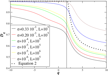
Figure 1: (Color online) The multifractal spectrum of uncoupled ($\alpha=0$) $T_{4}$’s as obtained numerically for finite $\epsilon$ and $N$. The solid vertical line is the line $q=2$. The dotted curve represents the analytical expression of the multifractal spectrum, Eq. (7).

II.2 Multifractal Spectra of Linearly Coupled Chebyshev Maps

Our interest in coupling Chebyshev maps results from the tendency of local interactions in systems with multiple components. In the current study we consider the simplest possible diffusive nearest neighbor coupling on a 1-D lattice with periodic boundary conditions. Namely, we assume a linear chain of units (’particles’) each of which is labelled by the index $i$. Each unit evolves according to Eq. (4) with additional, equal contributions from the left and right nearest neighbor particles. In the linear chain of size $L$, a coupling $\alpha$ is introduced so that the variable $x^{i}$ of the $i-th$ unit follows the recurrence relation

$$x_{n+1}^{i}=(1-\alpha)T_{4}(x_{n}^{i})+\frac{\alpha}{2}\left(T_{4}(x_{n+1}^{i})+T_{4}(x_{n-1}^{i})\right)$$ (10)

As initial conditions, a random distribution of $x_{0}^{i}\in\left[-1,1\right]$ is assumed. When Chebyshev maps are coupled on lattices the invariant 1-point densities are gradually deformed and singularities tend to smooth out groote:2006 . In particular, for $\alpha=1$ there are no singularities and $D_{q}=1,\forall q$, while the case $\alpha=0$ corresponds to a collection of independent $T_{4}$’s and the spectrum is given by the relation (7).

In Fig. 2 a series of multifractal spectra for different values of $\alpha$ are shown, for finite but small values of $\epsilon$. $L=10^{6}$ coupled $T_{4}$ maps are taken into account with $\epsilon=10^{-5}$ and $\epsilon=10^{-3}$ in Figs. 2a and 2b, respectively. In both cases, as $\alpha\to 1$, the multifractal spectrum is seen to become uniform. In Fig. 2b humps are observed due to finite size effects ($\epsilon$ as large as $10^{-3}$), for different values of $\alpha$. Note, in Fig. 2b, that the humps are more evident for higher values of the coupling constant $\alpha$. These $\alpha$-values are consistent with those that reproduce similar statistics as DNA sequences, as will be seen in the subsequent sections.

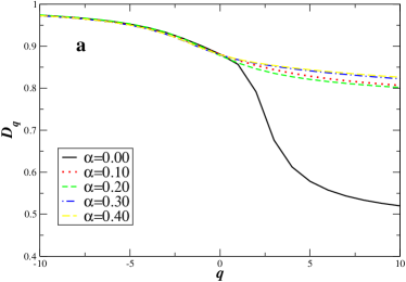
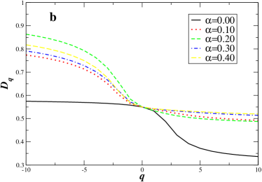
Figure 2: (Color online) a) Numerically obtained multifractal spectra of coupled $T_{4}$’s for various values of $\alpha$, $\epsilon=10^{-5}$. b) Humps in the multifractal spectra for coupled $T_{4}$ are observed for relatively large values of $\epsilon$ (here $\epsilon=10^{-3}$ is shown). $L=10^{6}$ in both a and b plots.

III Symbolic Sequences Resulting from CMLs

Having analyzed multifractal spectra that are directly associated with the local distribution of the state variables $x_{n}^{i}$ of the CML we now want to go a step further and produce symbol sequences from the CML. Comparing with the multifractal spectra of genomic sequences yu:2001 ; gutierrez:2001 ; su:2009 ; provata:2010 we note that there are certain similarities in the two spectra which suggests to explore the possibility of a certain chaotic CML processes to reproduce the most important genomic spectral features.

As a first step in this direction one has to reconstruct a symbolic sequence of 4 letters, based on the distribution of the local CML variable $x$. When constructing the artificial symbolic sequence one needs, at least, to respect the symbol concentrations of the original genomic sequence. If the genomic populations (mean concentrations) of the 4 nucleotides are denoted as $p_{A},p_{C},p_{G},p_{T}=1-p_{A}-p_{C}-p_{G}$ for Adenine, Cytosine, Guanine and Thymine, respectively, then the artificial $T_{4}$-based genomic sequence should contain the same frequency of the symbols. To achieve consistency between the genome basepair population and the symbolic sequence one needs to consider again the 1-point distribution $p(x)$ of the coupled $T_{4}$ map. The interval $[-1,1]$ is segmented into four subintervals $[-1,x_{1}]$ ,$[x_{1},x_{2}]$,$[x_{2},x_{3}]$ and $[x_{3},1]$, to accommodate the 4 basepairs. The values of $x_{1},x_{2}$ and $x_{3}$ were chosen to fulfill the basepair frequency constraints:

$$\begin{array}[]{lll}\int_{-1}^{x_{1}}dx\;p(x)=p_{A}\\ \int_{x_{1}}^{x_{2}}dx\;p(x)=p_{C}\\ \int_{x_{2}}^{x_{3}}dx\;p(x)=p_{G}\\ \int_{x_{3}}^{1}dx\;p(x)=p_{T}\\ \end{array}$$ (15)

Having fixed the segmentation values $[x_{1},x_{2},x_{3}]$, the $i$-th symbol $S_{n}^{i}$ of the artificial genomic sequence is chosen as

$$S_{n}^{i}=\left\{\begin{array}[]{lll}A&{\rm if}&-1<x_{n}^{i}\leq x_{1}\\ C&{\rm if}&x_{1}<x_{n}^{i}\leq x_{2}\\ G&{\rm if}&x_{2}<x_{n}^{i}\leq x_{3}\\ T&{\rm if}&x_{3}<x_{n}^{i}\leq 1\\ \end{array}\right.$$ (20)

Hence, a symbolic sequence $S_{n}(i),i=1,...L$ is produced which on the one hand carries the complexity of the CML and on the other hand respects the average concentrations of the DNA sequence under consideration, $(p_{A},p_{C},p_{G},p_{T}$).

In the search for a proper value of the coupling constant $\alpha$ which best describes the complexity of the genomic sequences, it is important to create CML-generated sequences of length comparable with the genomic ones. In the current study sequences of $L=10^{7}$ were produced to assimilate the chromosomal DNA. To avoid transient phenomena and to ensure that the CML Chebyshev maps have unfolded all their chaotic state space structure, we have chosen in the simulations to use the results produced after $n=5000$ iteration time steps. This is a safe choice because, normally, the CML sequences achieve their typical long-term behavior after about 20 iteration time steps. Averages over time steps $n$ were not performed. Rather, our aim was to analyze a given snapshot of symbols generated by the CML system that spatially had comparable length to that of the genomic sequence.

To locate the coupling constant which best reproduces the complexity of the genomic sequences, we calculated the multifractal spectra of the genomic sequence and compared it with the spectra of the CML-symbol sequences for various values of $\alpha$. The estimation of the multifractal exponents $D_{q}$ are based on the calculation of the probabilities $p(i_{1},i_{2},...i_{N})$ of finding blocks of symbols $i_{1},i_{2},...i_{N}$ along the sequence of size $L$, whereas $N$ is the linear size of the block provata:2010 ; beck:2010 :

$$D_{q}=\frac{1}{q-1}\lim_{N\to\infty}\frac{\log{\displaystyle\sum_{i_{1},i_{2},...i_{N}}[p(i_{1},i_{2},...i_{N})]^{q}}}{\log E},\>\>q\neq 1$$ (21)

$$D_{1}=\lim_{N\to\infty}\frac{\log{\displaystyle\sum_{i_{1},i_{2},...i_{N}}}p(i_{1},i_{2},...i_{N})\ln[p(i_{1},i_{2},...i_{N})]}{\log E},$$

In Eq. (III) $E$ represents the size (total number of configurations) of the statespace. In this representation the exponents $D_{q}$ represent the increase of the phase space when the size of the sequence (or window) increases. As an example we consider the homogeneous case, where

$$\left.\begin{array}[]{l}p(i_{1},i_{2},...i_{N})={1}/{s^{N}}\\ E=s^{N}\\ s=\>\>{\rm the\>\>number\>\>of\>\>symbols}=4\end{array}\right\}\Rightarrow D_{q}=1$$

as is expected for homogeneous sequences.

In Fig. 3 the multifractal spectrum of the human Chromosome 10 is plotted and compared with CML-$T_{4}$ for various values of $\alpha$. The calculations of the spectrum of chromosome 10 are based on evaluating all possible symbol sequences up to length $N=8$. This is considered as asymptotic behavior since the numerical result does not change for values $N>6$, as was previously shown in references yu:2001 ; provata:2010 . For the calculation of the various spectra based on the $T_{4}$ map the 1-point probabilities of the basepairs in chromosome 10 have been respected, via Eqs. (15) and (20), by choosing appropriate borders $x_{1},x_{2},x_{3}$ of the intervals. The observed 1-point probabilities for chromosome 10, used in this study, are provata:2010

$$p_{A}=0.291921,\>p_{C}=0.207966,$$ (24)

$$p_{G}=0.207859,\>p_{T}=0.292219.$$

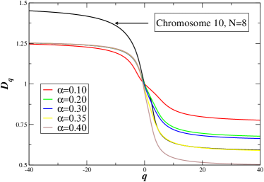
Figure 3: (Color online) The multifractal spectra for human Chromosome 10, with $N=8$ (black line) and CML-$T_{4}$’s for various values of the coupling constant $\alpha$.

A first look at Fig. 3, in the negative $q$ region, indicates that the coarse graining of the state space into 4 segments and the reduction of the continuous CML dynamics to a 4-symbol shift modifies the $T_{4}$ spectrum, producing $D_{q}>1$ for $q<0$. This is not surprising, since the multifractal spectrum presented in Eq. (7) relates to the statistics of the map and represents the frequency of iterates within the interval [-1,1], while Eq. (III) relates to the increase in the number of configurations in the symbolic sequence resulting from this map.

In addition, the deviation from unity for the negative $q$ spectrum is accentuated by the unequal frequencies of the four basepairs. In Fig. 4 the multifractal spectrum arising from the CML assimilating a random artificial DNA sequence with equal basepair distribution $p_{A}=p_{C}=p_{G}=p_{T}=0.25$ is compared to the case of non-equal basepair composition, Eq. (9). In the case of equal frequencies the CML process seems to create some rare configurations with small probability which tend to increase the $D_{q}$-values in the negative $q$ region.

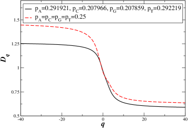
Figure 4: (Color online) The multifractal spectra for two artificial DNA sequences, produced via the $CML-T_{4}$. The coupling constant is $\alpha=0.35$. The dashed (red) line represents equal composition of the four basepairs $p_{A}=p_{C}=p_{G}=p_{T}=0.25$, while the solid (black) line represents composition given by Eq. (9).

Returning to Fig. 3 one observes that the closest approximation to the Chromosome 10 spectrum is achieved for $\alpha\sim 0.35$. This approximation is good only for positive $q-$values, which correspond to positive moments of the probability density. This means that configurations which are found often in the genome are well represented by the CML process $\alpha=0.35$, while rare configurations, which dominate the negative-$q$ spectra, are not accounted sufficiently in this approach.

In the next section, we will improve the model by ad hoc introducing a small number of rare configurations.

IV Taking into account Rare Oligonucleotides

To motivate the need for including rare oligonucleotide configurations, we first discuss some DNA functional issues related to the presence of specific rare segments. Long-time studies of the primary structure of higher eucaryotes and other organisms have revealed certain particularities related mainly to the functionality of DNA sequences. In particular, in coding sequences all combinations of the four letters are found with almost equal probability, without priority given to specific combinations. This is not true for the noncoding parts which comprise 95-97% of the human genome. In noncoding sequence repetitive elements are very common with only the Alu-(repetitive sequence) covering approximately 11% of the human genome alu:2008 . Other common elements which are often met in eucaryotes are the poly-A and poly-T chains. Likewise, sequences with specific functionality are very rare and they are only present for specific purposes in the noncoding region. Well known such examples are the TATAA box and the $GC$ and $CG$ complexes and multiple superpositions of them li:2002 ; bernaola:2004 ; li:2004 ; cheng:2005 ; messer:2006 ; katsaloulis:2002 ; katsaloulis:2006 ; han:2008 ; freudenberg:2009 . The presence of these complexes is associated with the presence of promoters, regulatory elements which designate the subsequent appearance of coding segments. These regulatory elements have the very specific task of “chemically attracting” the enzymes which will act on the closely following coding sequence in order to start the production of RNA which will finally lead to the production of the corresponding protein. Thus the presence of promoters (and their sequence structure) is very specific in the noncoding sequences and they are not abundantly found in the genome. Promoters are not the only sequences which are conserved for specific purposes. Other regulatory elements, such as the cis-acting and trans-acting elements, also have rare sequence structure.

From the above discussion it becomes clear that the structure of the noncoding segments, which dominate the genome of higher eucaryotes, is far from being uniform. The presence of rare configurations, which is mostly visible in the negative $q$ spectrum, needs to be taken into account for a proper modelling of the sequence dynamics. Rare sequences with specificity, which are not accounted for by the simple CML model presented in the previous section, will be thus considered ad-hoc in this section. This addition will mostly contribute to the negative $q-$ values of the multifractal spectrum, which is observed to be lower for the CML than for the human chromosomes.

We modify the dynamics by assuming that some of the rare symbol sequences generated by the CML become even less frequent by an external coupling mechanism (such as escape from the chaotic attractor). It is sufficient to artificially modify the probability of occurrence of a small fraction $\theta$ of configurations, eg. $\theta\sim 1/1000$, creating thus $\Theta=\theta\times E$ rarified configurations. The probability of occurrence of these rare configurations can be reduced to as much as $10^{-1}\times({\rm lowest-probability})$ for a much better approximation of the chromosomal multifractal spectra. These values are indicative and they depend weakly on the specific chromosome. In Fig. 5 the multifractal spectrum of human chromosome 10 is plotted together with CML-$T_{4}$ with coupling constant $\alpha=0.35$ and with modifications to include $\Theta=60$ rare configurations (blue line). For comparison the case of CML-$T_{4}$ with coupling constant $\alpha=0.35$ without rare configurations is also included (green dotted line). Because the modified configurations are few and rare, their contributions to the positive $q$ region of the multifractal spectrum is negligible. On the contrary, for negative $q$ they give an important contribution increasing significantly the $D_{q}$ values and good agreement is then achieved for both positive and negative $q$. Similar results are also obtained for the other human chromosomes, with adjustable values of $\alpha$ and $\theta$.

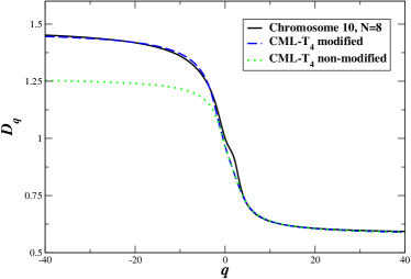
Figure 5: (Color online) The multifractal spectrum for human chromosome 10, with $N=8$ (black solid line), and CML-$T_{4}$ with coupling constant $\alpha=0.35$ modified with few rare configurations as described in the text (blue dashed line). The green dotted line depicts the CML-$T_{4}$ representation without rare configurations.

In Fig. 6 we plot the variable $\sigma$ which denotes the mean square deviation between the multifractal curve of chromosome 10 and CML-$T_{4}$’s modified with rare configurations for various values of $\alpha$.

$$\sigma^{2}(\alpha)=\frac{1}{N_{1}}\sum_{q=-N}^{N}\left(D_{q}^{CML}(\alpha)-D_{q}^{10}\right)^{2}$$ (25)

In Eq. (25) $D_{q}^{CML}(\alpha)$ denotes the multifractal exponent of order $q$ for the CML of $T_{4}$ with coupling constant $\alpha$, while $D_{q}^{10}$ denotes the corresponding multifractal exponent of order $q$ for chromosome 10. The sum runs from $-N$ to $N$ over positive and negative $q-$values at equal distance $\Delta$; $N_{1}=(2N+1)/\Delta$ is the total number of $q-$ values considered. Figure 6 shows that the smallest $\sigma$ value for chromosome 10 is found for $\alpha=0.35\pm 0.01$ and thus the coupled Chebyshev string with coupling constant $\alpha=0.35\pm 0.01$ best represents the correlations found in chromosome 10. Similar values are also obtained for the other human chromosomes.

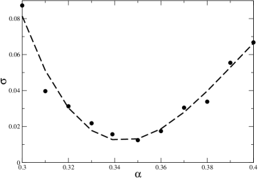
Figure 6: The deviation $\sigma$ (black circles) as a function of $\alpha$ between the multifractal spectra of human chromosome 10 and CML-$T_{4}$’s modified with rare configurations. The dotted line is a cubic fit to the data.

V Conclusion

The multifractal spectrum of CMLs has been determined using as a working example the 4-th order Chebyshev map $T_{4}$ diffusively coupled on a 1-D lattice with periodic boundary conditions. This choice of local map is particularly suited for our biological application since it corresponds to a shift of information encoded in 4 symbols, just as the DNA string encodes information using 4 nucleotides.

In the current study the CML was used to assimilate the correlated structure of genomic sequences, based on a comparison of the corresponding multifractal spectra. It was shown that the CML of $T_{4}$ can reproduce quite closely the multifractal spectrum of genomic sequences for positive $q-$values, while it deviates significantly for negative $q$. In particular, for human chromosome 10 (complete sequence) the best approximation for the positive $q$ spectrum is obtained for coupling constant value $\alpha=0.35$.

In an attempt to model both positive and negative $q-$ spectra of chromosomes as closely as possible, we consider the differences of the frequency representation of various functional units. One particular property of noncoding DNA is the presence of rare configurations (oligonucleotide sequences) which have specific functionality serving as promoters for the production of proteins or as regulatory elements. Such specific sequences are the TATAA-box, various $GC$-complexes and other elements which vary for different classes of organisms. We model these rare configurations by introducing an additional (artificial) escape process for the CML, which modifies the probabilities of certain rare sequences. If rare configurations representing these particular sequences are considered via an ad-hoc modification of the simulated distribution in the symbolic sequences resulting from the CML of $T_{4}$, then we see that both negative and positive $q$ multifractal spectra of genomic sequences are well approximated by the CMLs.

It is interesting to mention here that a good representation of the distribution of base pair sequences in DNA must be a superposition of (at least) two components. One of these components represents mostly the coding sequences and the second one contributes to the noncoding ones. This is in line with earlier studies of DNA sequences which have shown that the coding and noncoding parts follow different statistics, related to their different functionality scaling ; provata:2007 ; beck:2010 .

In the current study, as a representative example, the human chromosome 10 was investigated in detail and the optimum value of the corresponding coupling constant of the CML was determined. Likewise, additional studies not described here have shown similar qualitative and quantitative behavior for the other human chromosomes. Further studies are required to show if the same approach can be applied to different classes of organisms, where the ratio of lengths of coding/noncoding sequences takes on different values. In a future study it will be very interesting to explore the range of values of the coupling constant $\alpha$ and the rare configuration frequency $\theta$ that may characterize the different classes of organisms.

References

- (1) K. Kaneko, Progr. Theor. Phys. 72, 480 (1984)
- (2) R. Kapral, Phys. Rev. A 31, 3868 (1985)
- (3) A. Lemaitre and H. Chate, Europhys. Lett. 39, 377 (1997)
- (4) M.C. Mackey and J. Milton, Physica D 80, 1 (1995)
- (5) K. Kaneko (ed.), Theory and Applications of Coupled Map Lattices, Wiley, New York (1993)
- (6) C. Beck, Spatio-temporal Chaos and Vacuum Fluctuations of Quantized Fields, World Scientific, Singapore (2002)
- (7) W. Li and K. Kaneko, Europhys. Lett., 17, 655 (1992).
- (8) C. K. Peng, S. V. Buyldyrev, A. L. Goldberger, S. Havlin, F. Sciortino, M. I. Simons and H. E. Stanley, Nature, 356, 168 (1992).
- (9) R. F. Voss, Phys. Rev. Lett., 68, 3805 (1992).
- (10) R. N. Mantegna, S. V. Buldyrev, A. L. Goldberger, S. Havlin, C. K. Peng, M. Simons and H. E. Stanley, Phys. Rev. Letts., 73, 3169 (1994).
- (11) A. Provata, Y. Almirantis, Physica A, 247, 482 (1997); Y. Almirantis, A. Provata, J. Stat. Phys., 97, 233 (1999).
- (12) I. Grosse, P. Bernaola-Galvan, P. Carpena, R. Roman-Roldan, J. Oliver and H. E. Stanley, Phys. Rev. E, 65, 041905 (2002).
- (13) P. Carpena, P. Bernaola-Galvan, A. V. Coronado, M. Hackenberg and J.L Oliver, Phys. Rev. E 75, Art. No. 032903 (2007).
- (14) O. V. Usatenko, V. A. Yampol’skii, K. E. Kechedzhy and S. S. Mel’nyk Phys. Rev. E, 68, 061107 (2003).
- (15) V. Afreixo, P. J. S. G. Ferreira and D. Santos, Phys. Rev. E, 70,031910 (2004).
- (16) W. T. Li, Gene 300, 129-139 (2002).
- (17) P.Bernaola-Galvan, J.L. Oliver, P. Carpena, O. Clay and G. Bernardi, Gene, 333 121-133 (2004).
- (18) W. T. Li and D. Holste Fluctuation and Noise Letters 4, L453-L464 (2004).
- (19) J. Cheng and L. X. Zhang, Chaos, Solitons & Fractals 25, 339-346 (2005).
- (20) P. W. Messer and P. F. Arndt, Nucleic Acids Research 34, W692-W695 (2006).
- (21) P. Katsaloulis, T. Theoharis, A. Provata, Physica A, 316, 380 (2002); P. Katsaloulis, T. Theoharis, and A. Provata, J. Theor. Biol., 258, 18-26 (2009).
- (22) P. Katsaloulis, T. Theoharis, W. M. Zheng, B. L. Hao, A. Bountis, Y. Almirantis and A. Provata, Physica A, 366, 308-322 (2006).
- (23) L. Han, B. Su, W. H. Li and Z. M. Zhao, Genome Biology 9, Art. No. R79 (2008).
- (24) J. Freudenberg, M. Wang, Y. Yang and W.T. Li, BMC Bioinformatics, 10, 3805 (2009).
- (25) C. Beck and A. Provata (submitted).
- (26) C. Beck, Nonlinearity 4, 1131 (1991).
- (27) A. Hilgers, C. Beck, Physica D 156, 1 (2001).
- (28) S. Groote and C. Beck, Phys. Rev. E, 74, 046216 (2006).
- (29) C. Dettmann, Physica D 172, 88 (2002).
- (30) C. Beck and F. Schloegl, Thermodynamics of Chaotic Systems, Cambridge University Press, Cambridge (1993).
- (31) E. Ott, W. Withers and J.A. Yorke, J. Stat. Phys. 36, 697 (1984)
- (32) Z.-G. Yu, V. Anh and K.-S. Lau, Phys. Rev. E, 64, 031903 (2001).
- (33) A. Provata and P. Katsaloulis Phys. Rev. E, 81, 026102 (2010).
- (34) J.M. Gutierrez, M.A. Rodriguez and G. Abramson, Physica A, 300, 271-284 (2001).
- (35) Z.-Y. Su, T. Wu and S.-Y. Wang, Chaos, Solitons & Fractals, 40,1750-1765 (2009).
- (36) S. Groote and H. Veermae, Chaos, Solitons and Fractals, 41, 2354-2359 (2009).
- (37) E. A. Bennett, H. Keller, R. E. Mills,S. Schmidt, J. V. Moran, O. Weichenrieder, and S. E. Devine, Genome Res., 18, 1875-1883 (2008).
- (38) A. Provata, Th. Oikonomou, Physical Review E, 75 056102 (2007).