Geometric local invariants and pure three-qubit states

Abstract

We explore a geometric approach to generating local $SU(2)$ and $SL(2,\mathbb{C})$ invariants for a collection of qubits inspired by lattice gauge theory. Each local invariant or ‘gauge’ invariant is associated to a distinct closed path (or plaquette) joining some or all of the qubits. In lattice gauge theory, the lattice points are the discrete space-time points, the transformations between the points of the lattice are defined by parallel transporters and the gauge invariant observable associated to a particular closed path is given by the Wilson loop. In our approach the points of the lattice are qubits, the link-transformations between the qubits are defined by the correlations between them and the gauge invariant observable, the local invariants associated to a particular closed path are also given by a Wilson loop-like construction. The link transformations share many of the properties of parallel transporters although they are not undone when one retraces one’s steps through the lattice. This feature is used to generate many of the invariants. We consider a pure three qubit state as a test case and find we can generate a complete set of algebraically independent local invariants in this way, however the framework given here is applicable to generating local unitary invariants for mixed states composed of any number of $d$ level quantum systems. We give an operational interpretation of these invariants in terms of observables.

I Introduction

One approach to the study of entanglement is the identification of local invariants of a collection of quantum objects. With this approach we imagine the distant labs scenario in which $N$ spatially separated parties each hold one of the subsystems of an $N$ particle entangled state in their laboratory and they are free to make arbitrary transformations on their subsystem. One then looks for properties of the state that remain unchanged under such local transformations since, under the conditions that the transformations are unitary, entanglement is defined to be invariant. If the transformations belong to the group $SL(2,\mathbb{C})$ it turns out that entanglement, given by the well known measure concurrence, is also invariant. Rephrasing, we can write this scenario as a non-abelian lattice gauge theory; the arbitrary transformations are non-abelian local gauge transformations made on $N$ subsystems, the $N$ points of the lattice. Entanglement is a gauge invariant observable of the theory. It is this similarity that inspires our work.

Quite a lot is known about the local unitary invariants of simple entangled states. For example, for a pure state of a pair of qubits, there is essentially only one local invariant (not counting the normalization); it characterizes the amount of entanglement between the two qubits. For a pure state of three qubits, one can identify five independent local invariants, four of them expressing a different aspect of the state’s entanglement Carteret et al. (2000); Linden and Popescu (1998); Sudbery (2001). A fifth, the Kempe invariant, is not well understood Kempe (1999). There exist well known algebraic methods for generating invariants Grassl et al. (1998); Rains (2000); Barnum and Linden (2001); Teodorescu-Frumosu and Jaeger (2003); Osterloh and Siewert (2005); Osterloh (2010), but as the number of subsystems increases, the problem of identifying and interpreting independent invariants rapidly becomes very complicated.

Here we explore a different approach inspired by lattice gauge theory Münster and Walzl (2000). For a collection of $N$ qubits, we consider any closed path connecting some of the qubits, and we associate an invariant quantity with each such path. The invariant is formed by taking the trace of a transformation associated with the closed path, which in turn is the product of transformations associated with the individual two qubit links. Each of these ‘link-transformations’ is determined by the density matrix of the two qubits connected by the link. Because this density matrix will typically change if one performs a local operation on either of the two qubits, each link-transformation will also typically change under such local operations. The overall transformation around a closed loop can similarly change as one performs a local operation on the qubit that defines the loop’s starting point. However, the trace and the eigenvalues of the overall transformation do not change under any single-qubit operations. The trace is our invariant. In fact we will generate a few distinct invariants associated with the same path, by using different, but closely related, ways of making the correspondence between a two-qubit density matrix and a link-transformation i.e. one has the choice whether to apply a spin flip to each qubit in a given loop.

Other authors have explored relations between entanglement and gauge transformations, in the context of an analysis of the geometry of the set of states Mosseri and Dandoloff (2001); Bernevig and Chen (2003); Lévay (2004, 2005). Our approach is different in that the paths we consider are not paths in the set of states but discrete paths connecting the qubits themselves.

Thus our invariants are determined once we specify the correspondence between a two qubit density matrix and a link-transformation. The first rule we consider, and the one from which the other cases are derived, is this one:

$$M_{b}=\text{tr}_{a}\left[(M_{a}\otimes\mathbf{I}_{b})\rho_{ab}\right].$$ (1)

Here $\rho_{ab}$ is the two qubit density matrix in question, $M_{a}$ is a $2\times 2$ Hermitian matrix, and $M_{b}$ is its image under our transformation. (In section II we interpret this rule in terms of local observables.)

We hope that this geometric approach will ultimately prove useful in generating and classifying invariants of systems with many parts. In this paper we try out our ideas by applying them to a simple system of three qubits in a pure state. For that case, as indicated above, a natural set of $SU(2)$ invariants is already known. We ask whether this set, or an equivalent set, can be generated via our construction. We also ask whether the path-based approach sheds any light on the physical meaning of these invariants.

In the following section we introduce our basic path-based method of generating invariants. Section IV applies this idea to pure states of three qubits and makes the connection between the invariants generated by this method and the standard three qubit $SU(2)$ invariants that have been identified previously. In section V we show how to generate $SL(2,\mathbb{C})$ invariants by simply spin flipping each qubit in a loop. In section VI we give an operational interpretation of these invariants in terms of observables. Finally, we draw conclusions in section VII and outline how one would extend this approach to mixed states comprised of any number of qu$d$its.

II Path-based invariants

Our basic method of associating a transformation with each two qubit link is motivated by a thought experiment. Imagine many $N$ qubit systems, each having distinguishable qubits labeled $a$, $b$, $c$, $\ldots$, and each system being in the same quantum state $\rho$. We use $\rho$ to define a transformation from qubit $a$ to qubit $b$ as follows. On several copies of the state $\rho$, perform a general quantum measurement on qubit $a$, one of whose outcomes is represented by the operator $M_{a}$. (This operator is arbitrary except that it must be positive semi-definite and less than the identity so that it can be part of a legitimate measurement.) Now consider only those instances of qubit $a$ for which this particular outcome is actually achieved. In those cases, the state of qubit $b$ has been ‘collapsed’ into some state, typically mixed, even though qubit $b$ has not interacted with the measuring device. The final state of qubit $b$ is in fact proportional to

$$M_{b}=\text{tr}_{a}[(M_{a}\otimes\mathbf{I}_{b})\rho_{ab}],$$ (2)

where $\rho_{ab}$ is the original reduced density matrix of qubits $a$ and $b$ when the whole system is in state $\rho$. The normalization of $M_{b}$, that is, $\text{tr}M_{b}$, is equal to the probability of getting the outcome represented by $M_{a}$. In this way the density matrix $\rho_{ab}$ defines a linear transformation from operators on qubit $a$ to operators on qubit $b$, namely, the transformation that takes $M_{a}$ to $M_{b}$. It is convenient to represent this linear transformation as a matrix by writing $M_{a}$ and $M_{b}$ in terms of Pauli spin matrices. Let the four real numbers $m^{a}_{i}$, $i=0,\ldots,3$, be defined by

$$M_{a}=m^{a}_{0}\sigma_{0}+m^{a}_{1}\sigma_{1}+m^{a}_{2}\sigma_{2}+m^{a}_{3}\sigma_{3},$$ (3)

where $\sigma_{0}$ is the $2\times 2$ identity matrix and the other $\sigma_{i}$’s are the usual Pauli matrices, and let the components of $M_{b}$ be defined similarly. Then we can express our transformation as the $4\times 4$ matrix $S(b,a)$ such that

$$\mathbf{m}^{b}=S(b,a)\mathbf{m}^{a},$$ (4)

where $\mathbf{m}^{a}$ and $\mathbf{m}^{b}$ are column 4-vectors with components $m^{a}_{i}$ and $m^{b}_{i}$. Writing out eq. (2) explicitly in this operator basis, we have

$$\sum_{k}m^{b}_{k}\sigma^{b}_{k}=\text{tr}_{a}\left[\left(\sum_{i}m^{a}_{i}\sigma^{a}_{i}\otimes\mathbf{I}_{b}\right)\rho_{ab}\right].$$ (5)

Multiplying both sides by $\sigma_{j}^{b}$ and tracing over qubit $b$, we get an explicit expression for the components of the matrix $S(b,a)_{ji}$

$$S(b,a)_{ji}=\frac{1}{2}\text{tr}\left(\sigma^{a}_{i}\otimes\sigma^{b}_{j}\rho_{ab}\right)=\frac{1}{2}\langle\sigma^{a}_{i}\otimes\sigma^{b}_{j}\rangle.$$ (6)

So in this representation, the matrix representing our transformation from qubit $a$ to qubit $b$ is proportional to the spin correlation matrix. Our link-transformations are specified by the correlations between the qubits joined by the link.

We can now imagine repeating this process at qubit $b$. That is, starting with several pristine, unmeasured copies of the state $\rho$, we imagine performing a measurement on qubit $b$, one of whose outcomes is represented by the same operator $M_{b}$ that was the result of the first measurement. When this outcome is achieved, qubit $c$ will be collapsed into some mixed state proportional to $M_{c}$ defined as in eq. (2).

Continuing in this way around a closed loop, we finally collapse qubit $a$ into some state proportional to

$$M^{\prime}_{a}=\text{tr}_{z}\,[(M_{z}\otimes\mathbf{I}_{a})\rho_{za}],$$ (7)

where qubit $z$ is the one that precedes qubit $a$ at the end of the loop. In this way we have mapped, via the whole loop $\mathcal{C}$, an operator $M_{a}$ on the state space of qubit $a$ into another operator $M^{\prime}_{a}$ on the same space. The matrix representing this transformation is

$$S(a,a;\mathcal{C})=S(a,z)\cdots S(c,b)S(b,a).$$ (8)

In other words the overall transformation taking our initial measurement four vector $\mathbf{m}^{a}$ around the closed loop back to our new four vector $\mathbf{m}^{a^{\prime}}$ is

$$\mathbf{m}^{a^{\prime}}=S(a,a;\mathcal{C})\mathbf{m}^{a}.$$ (9)

As we show in the following section, the trace of this matrix is invariant under all single qubit unitary transformations. This trace is the invariant we associate with the given closed path. We present a graphical illustration of the idea in figure 1.

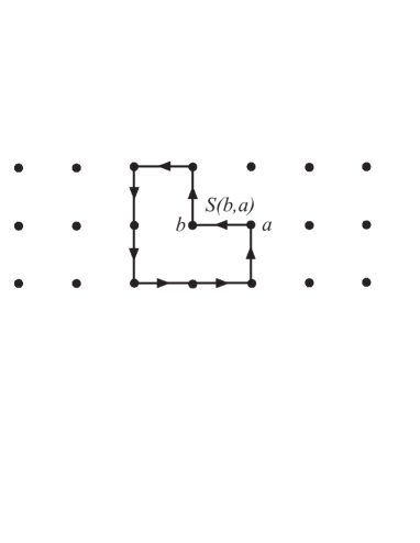
Figure 1: A schematic of our method of generating local invariants or ‘gauge invariants’ for a collection of quantum objects. The idea is inspired by lattice gauge theory with the lattice points representing qubits and the transformations $S(b,a)$ between lattice points $a$ and $b$ given by the correlations between qubits $a$ and $b$. Each distinct closed path or loop generates a local invariant.

Our basic transformation, eq. (2), is reminiscent of the transformation that would be associated with the two qubit state $\rho_{ab}$ by the Jamiołkowski isomorphism Jamiołkowski (1972), which provides a general correspondence between bipartite states and trace-preserving operations. The transformation defined by that isomorphism would be

$$M^{J}_{b}=2\text{tr}_{a}[(M^{T}_{a}\otimes\mathbf{I}_{b})\rho_{ab}].$$ (10)

That is, it would be normalized differently and it would require taking the transpose of the initial operator. The transpose is included in order to make the transformation a legitimate quantum operation—specifically, in order to make it completely positive. In contrast, the transformation defined by our eq. (2) need not be completely positive. We have chosen the form of eq. (2) as we have because our aim is not to define a quantum operation but rather to generate invariants. If we had included the transpose, the resulting $\text{tr}S(\mathcal{C})$ would not have been invariant. Moreover, even though our transformation is not a quantum operation, it does have a physical interpretation in terms of measurement.

Though introducing the transpose would spoil the invariance, there is a closely related operation that does not have this effect, namely, the spin flip. At any point along a closed path, we have the option of inserting a spin flip without destroying the invariance. In our thought experiment, this would mean that, having collapsed, say, qubit $b$ into the (subnormalized) state $M_{b}$, in our next step we would perform a measurement with an outcome represented by $\tilde{M}_{b}$, where the tilde represents the spin flip. That is,

$$\tilde{M}=\sigma_{2}M^{T}\sigma_{2}.$$ (11)

The effect of a spin flip on the vector $m$ representing $M$ in the Pauli basis is simply to multiply $m_{1}$, $m_{2}$, and $m_{3}$ by $-1$ and to leave $m_{0}$ unchanged. ($\sigma_{2}$ multiplies $m_{1}$ and $m_{3}$ by $-1$ while the transposition, equivalent to complex conjugation, multiplies $m_{2}$ by $-1$. The spin flip is anti-unitary and not a physical operation). That is, in this representation a spin flip is represented by the matrix $\eta$, the Minkowski metric;

$$\eta=\left(\begin{array}[]{cccc}1&0&0&0\\ 0&-1&0&0\\ 0&0&-1&0\\ 0&0&0&-1\end{array}\right).$$ (12)

We will label each of our invariants by the closed path that defines it, indicating with a tilde any site at which we have added a spin flip. Thus, for example, $I(a\tilde{b}c)$ is the invariant defined by

$$I(a\tilde{b}c)=\text{tr}\left\{S(a,c)S(c,b)\eta S(b,a)\right\}.$$ (13)

It is not hard to see that a spin flip indeed preserves the $SU(2)$ invariance. In the following section, we will show local transformations $\mathcal{U}$ become elements of $SO(3)$ acting only on the spatial dimensions of $S$, those with index values $1,2,3$ and not on the dimension associated with the identity. That is, they are block-diagonal matrices with a $1\times 1$ block and a $3\times 3$ block. Thus they commute with $\eta$ and therefore still cancel each other.

In fact we find that the inclusion of a spin flip on every qubit in a path results in not only an $SU(2)$ invariant but also a $SL(2,\mathbb{C})$ invariant, a group which contains $SU(2)$. The group $SL(2,\mathbb{C})$ represents the most general, local operations, such as Kraus operations, that one may perform on a qubit up to a positive constant less than unity. This stronger invariance is interesting as the well known entanglement measures concurrence and three-tangle exhibit this higher invariance Verstraete et al. (2001). We demonstrate this in the following section.

III Properties of link-transformations

III.1 Local operations

Suppose that on one qubit, say qubit $b$ for definiteness, we perform a general local operation, not necessarily unitary $\mathcal{U}_{b}$ i.e.

$$M_{b}=\text{tr}_{a}[(M_{a}\otimes\mathbf{I}_{b})(\mathbf{I}_{a}\otimes\mathcal{U}_{b})\rho_{ab}(\mathbf{I}_{a}\otimes\mathcal{U}_{b}^{\dagger})].$$ (14)

In a cycle that includes the links $a\rightarrow b$ and $b\rightarrow c$, this transformation would change both $S(b,a)$ and $S(c,b)$. For example, $S(b,a)_{ji}$ would be transformed into

$$\frac{1}{2}\langle\sigma^{a}_{i}\otimes({\mathcal{U}_{b}}^{\dagger}\sigma^{b}_{j}\mathcal{U}_{b})\rangle.$$ (15)

We can write this local operation on $b$ as the left action on $S(b,a)$,

$$S(b,a)\rightarrow U(b)S(b,a)$$ (16)

where the components of the new matrix $U(b)$ are given by

$$U(b)_{j_{1}j_{2}}=\frac{1}{2}\text{tr}\left({\mathcal{U}_{b}}^{\dagger}{\sigma^{b}_{j_{1}}}\mathcal{U}_{b}{\sigma^{b}_{j_{2}}}\right).$$ (17)

One can make a similar local operation, $\mathcal{U}_{a}$, simultaneously on qubit $a$ and find that

$$S(b,a)\rightarrow U(b)S(b,a)U(a)^{T}$$ (18)

where

$${U(a)^{T}_{i_{1}i_{2}}}=\frac{1}{2}\text{tr}\left({\mathcal{U}_{a}}{\sigma^{a}_{i_{1}}}{\mathcal{U}_{a}}^{\dagger}{\sigma^{a}_{i_{2}}}\right).$$ (19)

Under local operations we see that the link-transformations change in the same way as the parallel transporters in lattice gauge theories if the gauge group is an orthogonal group. The total transformation around the closed loop described by eq. (8), under arbitrary local operations, therefore becomes

$$S(a,a;\mathcal{C})=$$ (20)

$$U(a)S(a,z)U(z)^{T}\cdots U(c)S(c,b)U(b)^{T}U(b)S(b,a)U(a)^{T}.$$

Provided the local operations cancel each other, the trace of $S(a,a;\mathcal{C})$ is invariant under these operations. We now prove this fact specifically for $\mathcal{U}\in SU(2)$, that is $U^{T}U=\mathbf{I}$. Each of the components of $U^{T}U$ is given by

$$U_{l_{1}l_{2}}^{T}U_{l_{2}l_{3}}=\frac{1}{4}\text{tr}\left({\mathcal{U}}{\sigma_{l_{1}}}{\mathcal{U}}^{\dagger}{\sigma_{l_{2}}}\right)\text{tr}\left({\mathcal{U}}^{\dagger}{\sigma_{l_{2}}}\mathcal{U}{\sigma_{l_{3}}}\right).$$ (21)

Writing each of the $2\times 2$ matrices in index notation we have

$$\frac{1}{4}\mathcal{U}_{i_{1}i_{2}}(\sigma_{l_{1}})_{i_{2}i_{3}}{\mathcal{U}}^{\dagger}_{i_{3}i_{4}}(\sigma_{l_{2}})_{i_{4}i_{1}}{\mathcal{U}}^{\dagger}_{j_{1}j_{2}}(\sigma_{l_{2}})_{j_{2}j_{3}}\mathcal{U}_{j_{3}j_{4}}(\sigma_{l_{3}})_{j_{4}j_{1}}$$ (22)

where in the last equation the $l$ indices take the integer values $0\ldots 3$ and the $i$ and $j$ indices take the integer values $0$ and $1$. Summation is implied by a repeated index. We can use the relation

$$\frac{1}{2}\sum_{l=0}^{3}(\sigma_{l})_{i_{1}i_{2}}(\sigma_{l})_{i_{3}i_{4}}=\delta_{i_{1}i_{4}}\delta_{i_{2}i_{3}}$$ (23)

($\sum_{i=0}^{3}\sigma_{i}\otimes\sigma_{i}=SWAP$) and the unitary property of $\mathcal{U}$

$$\mathcal{U}_{i_{1}i_{2}}{\mathcal{U}}^{\dagger}_{i_{2}i_{3}}={\mathcal{U}}^{\dagger}_{i_{1}i_{2}}\mathcal{U}_{i_{2}i_{3}}=\delta_{i_{1}i_{3}}$$ (24)

to find

$$U_{l_{1}l_{2}}^{T}U_{l_{2}l_{3}}=\text{tr}\left(\sigma_{l_{1}}\sigma_{l_{3}}\right)=\delta_{l_{1}l_{3}}.$$ (25)

The remaining local unitary transformations, those made at the beginning (or end) of the loop cancel from the cyclic property of the trace. So the quantity $\text{tr }S(a,a;\mathcal{C})$ is indeed invariant under all local unitary transformations.

A simpler way to see that the local unitary transformations do indeed cancel is to recognize that an arbitrary unitary acting on a qubit when written in terms of the Pauli matrices is simply a three dimensional spatial rotation acting on the three spatial components $\sigma_{1}$, $\sigma_{2}$ and $\sigma_{3}$, that is, they are just rotations of the Bloch sphere. In other words the local operations $U(a)$, $U(b)$ acting on qubits $a$ and $b$ respectively in the $S(b,a)$ basis can be written explicitly as

$$U(b)S(b,a)U(a)^{T}=\begin{pmatrix}1&.\\ .&R_{b}\\ \end{pmatrix}\begin{pmatrix}s_{00}&s_{01}&s_{02}&s_{03}\\ s_{10}&s_{11}&s_{12}&s_{13}\\ s_{20}&s_{21}&s_{22}&s_{23}\\ s_{30}&s_{31}&s_{32}&s_{33}\\ \end{pmatrix}\begin{pmatrix}1&.\\ .&R_{a}^{T}\\ \end{pmatrix},$$ (26)

where $R_{b}$ and $R_{a}$ are $3\times 3$ rotation matrices, elements of $SO(3)$. That is, in the correlation matrix basis, $\mathcal{U}\in SU(2)$ become $U\in SO(3)$ due to the well known homomorphism $SU(2)\simeq SO(3)$ Arrighi and Patricot (2003). The components $s_{ji}$ are expectation values of the local spin measurements $\sigma_{i}^{a}$ and $\sigma_{j}^{b}$ made on $\rho_{ab}$. One can verify the form of $R_{a}$ and $R_{b}$ using eqns. (17) and (19).

In a similar way one can see that invariants where one performs a spin flip on each and every qubit are invariant under $\mathcal{U}\in SL(2,\mathbb{C})$ representing general local qubit operations up to a positive constant. The total transformation obtained by spin flipping every qubit can be explicitly written

$$S(\tilde{a},\tilde{a};\mathcal{C})=S(a,z)\eta\cdots\eta S(c,b)\eta S(b,a)\eta.$$ (27)

Under local operations $\mathcal{U}\in SL(2,\mathbb{C})$ we have seen from equations (16-19) that the correlation matrices $S$ transform as $S(b,a)\rightarrow U(b)S(b,a)U(a)^{T}$ thus we can form products such as $U(a)\eta U(a)^{T}$ from a transformation around a loop. Provided

$$U\eta U^{T}=\eta$$ (28)

our spin flipped quantities $I(\tilde{a}\tilde{b}\cdots\tilde{z})$ are invariant. In fact eq. (28) is the defining property of the group of Lorentz transformations, $SO^{+}(1,3)$, and due to the well known homomorphism $SL(2,\mathbb{C})\simeq SO^{+}(1,3)$ it indeed turns out that in the correlation matrix representation $\mathcal{U}\in SL(2,\mathbb{C})$ becomes $U\in SO^{+}(1,3)$ Arrighi and Patricot (2003). One can verify eq. (28) holds explicitly using eqs. (17) and (19). Therefore the spin flipped quantities $\text{tr}S(\tilde{a},\tilde{a};\mathcal{C})$ are invariant under local $SL(2,\mathbb{C})$ operations.

III.2 Directional property

One other useful property of the correlation matrices or link-transformations is simply demonstrated: The link-transformation taking $\mathbf{m}^{a}$ to $\mathbf{m}^{b}$, the real matrix $S(b,a)$, is the transpose of the link-transformation taking $\mathbf{m}^{b}$ to $\mathbf{m}^{a}$. That is

$$S(b,a)=S(a,b)^{T}.$$ (29)

This property is easily seen from eq. (6). We note that this is another property shared by the parallel transporters in lattice gauge theory, the parallel transporter that takes you from one lattice point to another is the transpose of the parallel transporter that takes you back provided the gauge group is $O(N)$. However, the parallel transporters have the additional feature that a loop not enclosing area is the identity, for example $U(a,b)U(b,a)=\mathbf{I}$. A similar expression for link-transformations does not hold. In fact we will make use of this property in the following section.

IV Identification of invariants

For any collection of qubits, one can consider the manifold representing the set of orbits of pure states under all local unitary transformations. That is, each point in the manifold corresponds to such an orbit. For a system of three qubits—we call them $a$, $b$, and $c$—it is known that the manifold of orbits is five dimensional Linden and Popescu (1998). (A quick but incomplete counting argument makes this result plausible. The eight-dimensional space of pure states can be parameterized by fourteen real numbers, if we fix the normalization and the overall phase. A generic orbit has nine degrees of freedom, because each of the three local unitaries has three real parameters. This leaves five parameters to specify the orbit itself.) Stating this in an alternative way for the case of a pure three qubit state, $|\psi\rangle$ is locally equivalent to $|\phi\rangle$ provided all local invariants specifying the orbit are equal . In the case of equality $|\psi\rangle$ and $|\phi\rangle$ have the same entanglement properties and one can obtain $|\phi\rangle$ from $|\psi\rangle$ simply by making local unitary transformations on each qubit.

Several authors have studied local invariants of pure three qubit states Coffman et al. (2000); Acìn et al. (2000); Carteret et al. (2000); Linden and Popescu (1998); Barnum and Linden (2001); Gingrich (2002); Leifer et al. (2004); Brun and Cohen (2001); Sudbery (2001). In particular, Sudbery Sudbery (2001) has identified a convenient set of algebraically independent invariants, each of which is a polynomial in the eight complex components of the vector $|\psi\rangle$. Not counting the normalization (which is Sudbery’s $I_{1}$), there are five of these invariants, the same as the number of dimensions:

$$I_{2}=\hbox{tr}[(\rho_{c})^{2}],\;\;I_{3}=\text{tr}[(\rho_{b})^{2}],\;\;I_{4}=\text{tr}[(\rho_{a})^{2}]$$

$$I_{5}=(\rho_{ab})_{ij^{\prime},i^{\prime}j}\,(\rho_{bc})_{jk^{\prime},j^{\prime}k}\,(\rho_{ca})_{ki^{\prime},k^{\prime}i}$$

$$I_{6}=(1/4)\tau_{abc}^{2}$$ (30)

where summation over repeated indices is implied in the definition of $I_{5}$. Here each index takes the values 0 and 1, and we have used the letters $i$, $j$, and $k$ to refer to qubits $a$, $b$, and $c$ respectively. The Kempe invariant $I_{5}$ Kempe (1999) can be written in several different ways, the above form being most convenient for our purpose. The quantity $\tau_{abc}$, is the 3-tangle which measures a kind of three-way entanglement characteristic of the GHZ state $(1/\sqrt{2})(|000\rangle+|111\rangle)$ Coffman et al. (2000). If we write $|\psi\rangle$ in terms of the standard basis states as $|\psi\rangle=\sum a_{ijk}|ijk\rangle$, then the invariant $I_{6}$ can be expressed as

$$I_{6}=\left|\epsilon_{i_{1}i_{2}}\epsilon_{i_{3}i_{4}}\epsilon_{j_{1}j_{2}}\epsilon_{j_{3}j_{4}}\epsilon_{k_{1}k_{3}}\epsilon_{k_{2}k_{4}}a_{i_{1}j_{1}k_{1}}a_{i_{2}j_{2}k_{2}}a_{i_{3}j_{3}k_{3}}a_{i_{4}j_{4}k_{4}}\right|^{2},$$ (31)

where $\epsilon_{ij}$ is the antisymmetric tensor in two dimensions.

The invariants listed in eq. (IV) are not complete in the sense of determining a unique orbit. In particular, these invariants do not distinguish between a state and its complex conjugate, which may well lie on different orbits. Because $I_{1}$ - $I_{6}$ are real

$$I_{i}(|\psi\rangle)=I_{i}(|\psi\rangle^{*}).$$ (32)

As reported by Acìn et al. Acìn et al. (2001), Grassl has shown that this ambiguity can be removed by including a single binary invariant based on a complex twelfth-degree polynomial in the amplitudes $a_{ijk}$.

We now ask whether the invariants in eq. (IV) can be generated via the formalism of section II. The first three can indeed be expressed quite simply in this way. For example,

$$I(ab) = \text{tr}\left\{S(a,b)S(b,a)\right\}$$ (33)

$$= \sum_{ij}\text{tr}\left[\left(\frac{\sigma_{i}^{a}\otimes\sigma_{j}^{b}}{2}\right)\rho_{ab}\right]^{2}$$

$$= \text{tr}[(\rho_{ab})^{2}]=\text{tr}[(\rho_{c})^{2}]=I_{2}.$$

The last line follows from the fact that the operators $(\sigma_{i}^{a}\otimes\sigma_{j}^{a})/2$ constitute a complete orthonormal basis for the space of $4\times 4$ matrices.

The Kempe invariant $I_{5}$ fits particularly well into our scheme. As we now show, this invariant is simply

$$I_{5}=I(abc)=\text{tr}\left\{S(a,c)S(c,b)S(b,a)\right\}.$$ (34)

To see this, we start with the following expression for $I(abc)$:

$$\frac{1}{8}\text{tr }\left[\left(\sigma^{a}_{l}\otimes\sigma^{b}_{m}\right)\rho_{ab}\right]\text{tr }\left[\left(\sigma^{b}_{m}\otimes\sigma^{c}_{n}\right)\rho_{bc}\right]\text{tr }\left[\left(\sigma^{c}_{n}\otimes\sigma^{a}_{l}\right)\rho_{ca}\right]$$ (35)

in which summation over $l$, $m$, and $n$ is implied. This summation considerably simplifies the expression, because of eq. (23). This relation tells us how to connect up the indices of the three density matrices, and we obtain the interlocking pattern that we saw in eq. (IV):

$$I(abc)=(\rho_{ab})_{ij^{\prime},i^{\prime}j}\,(\rho_{bc})_{jk^{\prime},j^{\prime}k}\,(\rho_{ca})_{ki^{\prime},k^{\prime}i}=I_{5}.$$ (36)

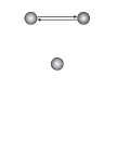
(a) $I(ab)$

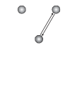
(b) $I(bc)$

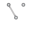
(c) $I(ca)$

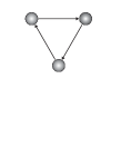
(d) $I(abc)$

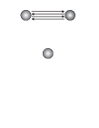
(e) $I(abab)$

Figure 2: Graphical representations of the closed paths giving the set of polynomial local $SU(2)$ invariants for pure states of three qubits.

Of the set of invariants that Sudbery identifies, the only one remaining is $I_{6}$, a degree-eight polynomial in the components $a_{ijk}$ and their conjugates which is proportional to the square of the 3-tangle. $I_{6}$ is also invariant under $SL(2,\mathbb{C})$ unlike $I_{1}$ - $I_{5}$ which do not have this higher invariance. Our formalism does not produce $I_{6}$ directly, though we can easily generate a different polynomial of degree eight that is likewise algebraically independent of the first four invariants. It is defined by any path that cycles twice between two of the qubits, that is, any of the invariants

$$I(abab)=I(bcbc)=I(caca).$$ (37)

One can write down this invariant directly in terms of the reduced density matrices $\rho_{ab}$ and $\rho_{ba}$ (which are related to each other by the swap operation that interchanges the two qubits), following precisely the pattern of index connections that we see in eq. (36). Now, however, because the same two-step path is repeated, we use subscripts 1 and 2 on the indices to distinguish the two round-trips.

$$I(abab)=\text{tr}\left\{S(a,b)S(b,a)S(a,b)S(b,a)\right\}$$ (38)

$$= (\rho_{ab})_{i_{1}j^{\prime}_{1},i^{\prime}_{1}j_{1}}(\rho_{ba})_{j_{1}i^{\prime}_{2},j^{\prime}_{1}i_{2}}(\rho_{ab})_{i_{2}j^{\prime}_{2},i^{\prime}_{2}j_{2}}(\rho_{ba})_{j_{2}i^{\prime}_{1},j^{\prime}_{2}i_{1}}.$$

We can alternatively write out this invariant in terms of the components $a_{ijk}$:

$$I(abab) = a_{i_{1}j_{2}k_{1}}a^{*}_{i_{2}j_{1}k_{1}}a_{i_{4}j_{1}k_{2}}a^{*}_{i_{3}j_{2}k_{2}}$$ (39)

$$\times a_{i_{3}j_{4}k_{3}}a^{*}_{i_{4}j_{3}k_{3}}a_{i_{2}j_{3}k_{4}}a^{*}_{i_{1}j_{4}k_{4}}.$$

In this latter form it is clear that the invariant is symmetric under permutations of the qubits: by permuting the factors of $a$ and $a^{*}$, one can interchange the roles of the $i$, $j$, and $k$ indices.

To show that the invariants we have identified are algebraically independent, it is sufficient to show that their gradients at any point, together with the gradient of the normalization invariant $I_{1}=a_{ijk}a^{*}_{ijk}$, constitute a linearly independent set of vectors Sudbery (2001). One finds that this is indeed the case. So we now have the following list of path-based invariants, not quite identical to Sudbery’s but no less complete:

$$I(ab) = \text{tr}\left\{S(a,b)S(b,a)\right\},$$

$$I(bc) = \text{tr}\left\{S(b,c)S(c,b)\right\},$$

$$I(ca) = \text{tr}\left\{S(c,a)S(a,c)\right\},$$

$$I(abc) = \text{tr}\left\{S(a,c)S(c,b)S(b,a)\right\},$$

$$I(abab) = \text{tr}\left\{S(a,b)S(b,a)S(a,b)S(b,a)\right\},$$ (40)

the last one being symmetric under permutations of the three qubits even though the path it is based on is not. The three kinds of path we have used in constructing our invariants are illustrated in figure 2.

Notice that our construction provides an interpretation of the Kempe invariant $I(abc)=I_{5}$. In our measurement scenario, in which each successive measurement collapses the state of the next qubit, the Kempe invariant is the trace of the transformation that results from following the triangular path through all three qubits. Recall that at each stage in this measurement scenario, the trace of the new $M$ matrix is equal to the probability of getting the desired outcome. Thus, the resulting invariant tends to be larger if the collapsed state at each step is strongly represented in the original reduced density matrix of the qubit in question. The most extreme example of this kind of consistency is the case of a completely factorable state, in which the collapsed state must be proportional to the original pure state of the given qubit. And indeed, the Kempe invariant is largest when the state is fully factorable ($I(abc)=1$). One can also show the Kempe invariant takes its minimal value for the W state $|001\rangle+|010\rangle+|100\rangle$ at $I(abc)=2/9$ Osterloh (2010).

V Local invariants using the spin flip

In section IV we provided a complete set of algebraically independent local $SU(2)$ invariants by considering different closed paths around the lattice. In this section we again consider closed paths around the lattice but this time including the spin flip operation on every qubit lifting the invariance of the quantities produced to $SL(2,\mathbb{C})$.

From the $SU(2)$ invariant list, it turns out that we can replace $I(ab)$, $I(bc)$, and $I(ca)$ with $I(\tilde{a}\tilde{b})$, $I(\tilde{b}\tilde{c})$, and $I(\tilde{c}\tilde{a})$; the invariants are still independent. Moreover, these ‘flipped’ invariants can also be interpreted in terms of entanglement. One finds that

$$I(\tilde{a}\tilde{b})=\text{tr}\left[\rho_{ab}\tilde{\rho}_{ab}\right]=\tau_{ab}+\frac{1}{2}\tau_{abc}$$

$$I(\tilde{b}\tilde{c})=\text{tr}\left[\rho_{bc}\tilde{\rho}_{bc}\right]=\tau_{bc}+\frac{1}{2}\tau_{abc}$$

$$I(\tilde{c}\tilde{a})=\text{tr}\left[\rho_{ca}\tilde{\rho}_{ca}\right]=\tau_{ca}+\frac{1}{2}\tau_{abc}$$ (41)

Here $\tilde{\rho}=(\sigma_{2}\otimes\sigma_{2})\rho^{T}(\sigma_{2}\otimes\sigma_{2})$ is the spin flipped state of the two qubits, and $\tau_{ab}$ is the tangle between qubits $a$ and $b$, a measure of their pairwise entanglement (it is the square of the concurrence) Wootters (1998). The completely flipped version of $I(abab)$, that is, $I(\tilde{a}\tilde{b}\tilde{a}\tilde{b})$, likewise produces a non-trivial invariant but it is not algebraically independent of $I(\tilde{a}\tilde{b})$, $I(\tilde{b}\tilde{c})$, and $I(\tilde{c}\tilde{a})$. A natural eighth order $SL(2,\mathbb{C})$ invariant is given by the determinant of any of the link-transformations, for example:

$$\det\left[S(a,b)\right]=-\frac{1}{16}\tau_{ab}(\tau_{ab}+\tau_{abc}).$$ (42)

One can see the determinant of the link-transformations is indeed $SL(2,\mathbb{C})$ invariant from the way the link-transformations change under arbitrary local $SL(2,\mathbb{C})$ transformations (eq. (18)) and the property of the determinant $\det(AB)=\det(A)\det(B)$. We can show this invariant is algebraically independent of $I(\tilde{a}\tilde{b})$, $I(\tilde{b}\tilde{c})$, and $I(\tilde{c}\tilde{a})$ using the same methods of section IV.

So far we have a set of four $SL(2,\mathbb{C})$ invariants. They tell us about the entanglements in the state since one can reconstruct the amounts of entanglement, $\tau_{ab}$, $\tau_{bc}$, $\tau_{ac}$ and $\tau_{abc}$ from just these four invariants. For example, the 3-tangle can be expressed as

$$\tau_{abc}=2\sqrt{16\det S(a,b)+I(\tilde{a}\tilde{b})^{2}}.$$ (43)

Even though the three qubit labels do not enter this expression symmetrically (there is no explicit reference to qubit $c$), the 3-tangle is symmetric under permutations of the qubits. Similar expressions can be written for the 2-tangles.

These four amounts of entanglement do not form a complete set of algebraically independent invariants. To complete this set we could use the $SU(2)$ Kempe invariant which one can verify is algebraically independent of the four tangles, however we would also like an invariant with $SL(2,\mathbb{C})$ local invariance. A natural choice of loop is the one that gave the Kempe invariant. Strangely enough, the completely flipped version of the Kempe invariant, that is, $I(\tilde{a}\tilde{b}\tilde{c})$, turns out to be exactly zero for all pure three qubit states as we prove in the following subsection.

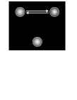
(a) $I(\tilde{a}\tilde{b})$

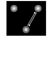
(b) $I(\tilde{b}\tilde{c})$

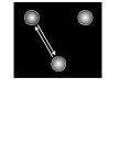
(c) $I(\tilde{c}\tilde{a})$

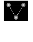
(d) $I(\tilde{a}\tilde{b}\tilde{c})$

(e) $\det(S(a,b))$

Figure 3: Graphical representations of the closed paths giving the set of polynomial local $SL(2,\mathbb{C})$ invariants for pure states of three qubits. Notice that $I(\tilde{a}\tilde{b}\tilde{c})$, the flipped Kempe invariant, is the only closed path to enclose area. It is also always equal to zero.

V.1 Proof of $I(\tilde{a}\tilde{b}\tilde{c})=0$ for any pure three qubit state.

From the definition of $I(\tilde{a}\tilde{b}\tilde{c})$, one finds directly that

$$\begin{split}I(\tilde{a}\tilde{b}\tilde{c})=&1-\text{tr}(\rho_{a}^{2})-\text{tr}(\rho_{b}^{2})-\text{tr}(\rho_{c}^{2})\\ &+\text{tr}[(\rho_{a}\otimes\rho_{b})\rho_{ab}]+\text{tr}[(\rho_{b}\otimes\rho_{c})\rho_{bc}]\\ &+\text{tr}[(\rho_{a}\otimes\rho_{c})\rho_{ac}]-I_{5}.\end{split}$$ (44)

Sudbery Sudbery (2001) showed that Kempe’s invariant can also be written as

$$\begin{split}I_{5}&=3\text{tr}[(\rho_{a}\otimes\rho_{b})\rho_{ab}]-\text{tr}(\rho_{a}^{3})-\text{tr}(\rho_{b}^{3})\\ &=3\text{tr}[(\rho_{b}\otimes\rho_{c})\rho_{bc}]-\text{tr}(\rho_{b}^{3})-\text{tr}(\rho_{c}^{3})\\ &=3\text{tr}[(\rho_{a}\otimes\rho_{c})\rho_{ac}]-\text{tr}(\rho_{a}^{3})-\text{tr}(\rho_{c}^{3}).\end{split}$$ (45)

Using these relations we can rewrite $I(\tilde{a}\tilde{b}\tilde{c})$ as

$$\begin{split}I(\tilde{a}\tilde{b}\tilde{c})=&1-[\text{tr}(\rho_{a}^{2})+\text{tr}(\rho_{b}^{2})+\text{tr}(\rho_{c}^{2})]\\ +&\frac{2}{3}[\text{tr}(\rho_{a}^{3})+\text{tr}(\rho_{b}^{3})+\text{tr}(\rho_{c}^{3})].\end{split}$$ (46)

This last expression is a function only of the trace of powers of the single-qubit density matrices. The Cayley-Hamilton theorem for any $2\times 2$ matrix $X$ is

$$X^{2}-\text{tr}(X)X+\det(X)\mathbf{I}=0.$$ (47)

Multiplying this expression by $X$, taking the trace, and then using the fact that for a single qubit, $\det\rho=(1/2)(1-\text{tr}\rho^{2})$, we obtain the relation

$$1/3-\text{tr}(\rho^{2})+(2/3)\text{tr}(\rho^{3})=0,$$ (48)

which together with eq. (46) shows that $I(\tilde{a}\tilde{b}\tilde{c})=0$.

VI Operational interpretation of invariants

Going back to our original thought experiment in section II we can obtain a rigorous operational interpretation of our invariants as follows if we drop the restriction that $M_{a}$ is positive but still Hermitian. In other words $M_{a}$ represents an observable rather than a measurement outcome. If we relax the positivity our invariant can be thought of as the average fidelity between our initial observable outcome $M_{a}$ and our final observable outcome $M_{a}^{\prime}$ resulting from the transform around the loop associated to the particular invariant, $I(\mathcal{C})$. The average is taken over all possible initial outcomes $M_{a}$ with a fixed size. Making this idea more precise, we have

$$I(\mathcal{C})\propto\langle\text{tr}(M_{a}^{\dagger}M_{a}^{\prime})\rangle,$$ (49)

where the brackets $\langle.\rangle$ denote the average.

The constraint on $M_{a}$’s size is given by

$$\text{tr}(M_{a}^{\dagger}M_{a})=2k^{2}.$$ (50)

In terms of the Pauli operator basis, this condition can be written as

$$\text{tr}(M_{a}^{\dagger}M_{a})=2\sum_{i=0}^{3}(m_{i}^{a})^{2}=2k^{2}.$$ (51)

The $m_{i}^{a}$ must be real for $M_{a}$ to be Hermitian and represent the outcome of an observable. Similarly we can write the outcome on $a$ following the loop $\mathcal{C}$ in the Pauli operator basis as (dropping the sub- and superscript $a$)

$$M^{\prime}=\sum_{i=0}^{3}m_{i}^{\prime}\sigma_{i}$$ (52)

where

$$m_{i}^{\prime}=S(\mathcal{C})_{ij}m_{j}.$$ (53)

$S(\mathcal{C})$ is the total transformation around the loop.

We can substitute these expressions into the equation for the fidelity between transformed and initial observable outcomes to give

$$\text{tr}(M^{\dagger}M^{\prime}) = 2\sum_{i=0}^{3}m_{i}m_{i}^{\prime}$$ (54)

$$= 2\sum_{i,j=0}^{3}m_{i}S(\mathcal{C})_{ij}m_{j}.$$

Our invariant $I(\mathcal{C})$ is given by the elements $S(\mathcal{C})_{ii}$ and therefore we want to find an expression solely in terms of these elements.

We now average this fidelity. Since eq. (50) is the equation of a 3-sphere with radius $k$ we can perform the average over the surface of the 3-sphere. Writing the $m_{i}$ in hyper-spherical coordinates we have

$$m_{0} = k\cos\phi_{1}$$

$$m_{1} = k\sin\phi_{1}\cos\phi_{2}$$

$$m_{2} = k\sin\phi_{1}\sin\phi_{2}\cos\phi_{3}$$

$$m_{3} = k\sin\phi_{1}\sin\phi_{2}\sin\phi_{3}.$$ (55)

We can now compute the average fidelity in terms of these coordinates. It is given by

$$\langle\text{tr}\left(M^{\dagger}M^{\prime}\right)\rangle=\frac{2}{A}\sum_{i,j=0}^{3}S(\mathcal{C})_{ij}\int_{\mathcal{S}}m_{i}m_{j}d\mathcal{S}.$$ (56)

$\mathcal{S}$ is the entire surface of the 3-sphere, $d\mathcal{S}=k^{2}\sin^{2}\phi_{1}\sin\phi_{2}d\phi_{1}d\phi_{2}d\phi_{3}$ is the area element and $A=2\pi^{2}k^{2}$ is its total surface area. One finds that

$$\frac{2}{A}\int_{\mathcal{S}}m_{i}m_{j}d\mathcal{S}=\frac{k^{2}}{2}\delta_{ij}$$ (57)

and we obtain our desired result

$$\langle\text{tr}(M^{\dagger}M^{\prime})\rangle=\frac{k^{2}}{2}I(\mathcal{C}).$$ (58)

One can also average over all observable sizes (or strengths) $k$ to obtain the same result up to a constant. The surface integral over the sphere now becomes a volume integral over the 3-ball. We also note we can choose $M_{a}$ to be an element of $SU(2)$. That is, a unitary that does not have to be Hermitian. In this case $k=1$ and the average is over the three Euler angles describing a element of this group. For $SU(2)$ $m_{0}$ is real and $m_{1}$, $m_{2}$, $m_{3}$ are purely imaginary. The proof goes through in the same way.

VII Conclusions

In this paper we have presented a geometric approach to constructing quantities that are invariant under local $SU(2)$ and $SL(2,\mathbb{C})$ transformations. Our basic construction corresponds to a scenario in which a measurement outcome on each particle along a closed path defines the state of the next particle. We have seen that one can produce in this way an algebraically independent set of five invariants for a pure state of three qubits, almost identical to the set of invariants identified by Sudbery. One of these quantities, the Kempe invariant, has been difficult to interpret as an amount of entanglement. In our construction, though, it is the one that emerges the most naturally. Unlike the other four invariants, the Kempe invariant $I_{5}=I(abc)$ corresponds to a path that ‘encloses area’ in the sense that one does not retrace one’s steps. This property sets the Kempe invariant apart from the others. Notice that for an area enclosing path, one needs at least three qubits. In a future paper we will exploit this area enclosing property and the existence of a special form of a polar decomposition for correlation matrices to find quantities much more analogous to lattice gauge field theories. The gauge group will turn out to be the group of Lorentz transformations and has an operational interpretation in terms of general local qubit operations. The invariants, the Wilson loops, in this construction, will be related to the curvature of the correlation space Williamson et al. (2011).

We have also provided an operational interpretation of the invariants, including the Kempe invariant, in terms of the average fidelity between initial and transformed observable outcomes.

We have concentrated on pure three qubit states as a test ground for our ideas, however there is nothing specific here about the numbers of qubits of our quantum state. Neither is there any requirement for the state to be pure or for the subsystems to be two level. The framework presented here can be applied to any qu$d$it state to generate local unitary invariants. To make this generalization, one replaces the Pauli matrices specific for qubits, by the generalized Gell-Mann matrices $\lambda_{i}$, an orthonormal basis for the (real) $(d^{2}-1)$ dimensional vector space of traceless hermitian $d\times d$ matrices with the inner product $(X,Y)=\text{tr}(XY)$. For $\mathcal{U}\in SU(d)$, the components of the local operation in the correlation matrix basis, $U_{ij}=\text{tr}(\mathcal{U}\lambda_{i}\mathcal{U}^{\dagger}\lambda_{j})$ is a special orthogonal matrix in $SO(d^{2}-1)$, representing $\mathcal{U}$ in the $(d^{2}-1)$ dimensional (adjoint) representation of $SU(d)$. More precisely, the orthogonal matrices with components $U_{ij}$ form a subgroup of $SO(d^{2}-1)$, being the homomorphic image of $SU(d)$ called the adjoint group, which is the quotient of $SU(d)$ by its centre, the subgroup of matrices $\omega\mathbf{I}_{d}$ where $\omega$ is a $d$th root of unity. Thus, the property $U^{T}U=\mathbf{I}_{d}$ still holds and $\text{tr}S(\mathcal{C})$ is invariant under $SU(d)$. However, for $SL(d,\mathbb{C})$ the connection with a Lorentz group only works for $d=2$.

We have seen for three pure qubits that only one area enclosing path exists, but as the number of qubits increases, there should be many more Kempe like quantities, since there will be many more paths that enclose area. Our original construction, on the other hand, produces many more invariants even for three qubits, because it makes critical use of the ‘shrinking’ component of the transformation defined by the spin correlation matrix.

One caveat with this approach as it stands is that we have only used the information contained in the two qubit density matrices. For states with large numbers of qubits one cannot obtain a full set of invariants since too much information about the overall state is lost when tracing out all but the two qubits in each link. This approach could be extended by considering contractions of the full correlation tensor. For example, an $N$ qubit system is described by a real tensor $S_{i_{1}j_{2}\cdots z_{N}}$ where $i_{1},j_{2},\cdots,z_{N}$ take the values $0,1,2,3$. It would be interesting to find an operational interpretation of contractions of these $N-$tensors.