Dust-correlated cm-wavelength continuum emission on translucent clouds $\zeta$ Oph and LDN 1780

Abstract

The diffuse cm-wave IR-correlated signal, the “anomalous” CMB foreground, is thought to arise in the dust in cirrus clouds. We present Cosmic Background Imager (CBI) cm-wave data of two translucent clouds, $\zeta$ Oph and LDN 1780 with the aim of characterising the anomalous emission in the translucent cloud environment.

In $\zeta$ Oph, the measured brightness at 31 GHz is $2.4\sigma$ higher than an extrapolation from 5 GHz measurements assuming a free-free spectrum on 8 arcmin scales. The SED of this cloud on angular scales of 1^∘ is dominated by free-free emission in the cm-range. In LDN 1780 we detected a 3 $\sigma$ excess in the SED on angular scales of 1^∘ that can be fitted using a spinning dust model. In this cloud, there is a spatial correlation between the CBI data and IR images, which trace dust. The correlation is better with near-IR templates (IRAS 12 and 25 $\mu$m) than with IRAS 100 $\mu$m, which suggests a very small grain origin for the emission at 31 GHz.

We calculated the 31 GHz emissivities in both clouds. They are similar and have intermediate values between that of cirrus clouds and dark clouds. Nevertheless, we found an indication of an inverse relationship between emissivity and column density, which further supports the VSGs origin for the cm-emission since the proportion of big relative to small grains is smaller in diffuse clouds.

1 Introduction

Amongst the challenges involved in the study of Cosmic Microwave Background (CMB) anisotropies is the subtraction of Galactic foreground emission. The detailed study of these foregrounds led to the discovery of a new radio-continuum mechanism in the diffuse interstellar medium (ISM). It was first detected by the Cosmic Background Explorer as a diffuse all-sky dust-correlated signal with a flat spectral index between 31 and 53 GHz (Kogut et al., 1996a, b). With ground based observations, Leitch et al. (1997) observed high Galactic latitude clouds and detected an excess at 14.5 GHz that, because of a lack of H$\alpha$ emission, could not be accounted for by free-free with typical temperatures ($T\sim 10^{4}$K).

Figure 1: ($u,v$) coverage of the CBI (left) and CBI2 (right) in the configurations used for the observations of $\zeta$ Oph on the left and LDN 1780 on the right. Axes are in units of wavelength ($\lambda$).

Different emission mechanisms have been proposed for the anomalous emission, such as spinning dust (Draine & Lazarian, 1998a, b), magnetic dust (Draine & Lazarian, 1999), hot (T$\sim$10⁶ K) free-free (Leitch et al., 1997) and hard synchrotron radiation (Bennett et al., 2003). To date, the evidence favours the spinning dust grain model (Finkbeiner et al., 2004; de Oliveira-Costa et al., 2004; Watson et al., 2005; Casassus et al., 2006, 2008; Castellanos et al., 2010) in which very small grains (VSGs) with a non-zero dipole moment rotating at GHz frequencies emit cm-wave radiation. The emission has its peak at $\sim$20-40 GHz and the model predicts that it is dominated by the smallest grains, possibly polycyclic aromatic hydrocarbons (PAHs). Ysard et al. (2010) found a correlation across the whole sky using WMAP data between 23 GHz maps and IRAS 12 $\mu$m, which supports the VSG origin for the cm-wave emission.

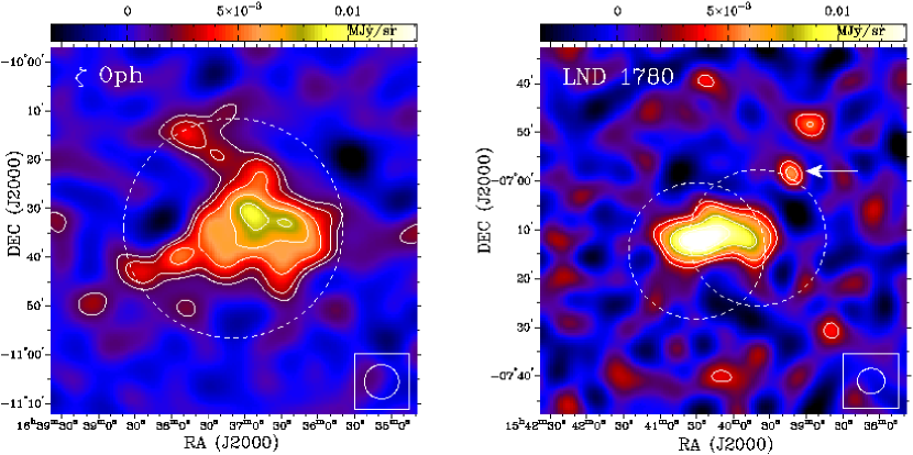
Figure 2: CLEANed 31 GHz images of $\zeta$ Oph (left) and LDN 1780 (right). Contours are 10, 30, 50, 70, 90% of the peak brightness, which is $9\times 10^{-3}$ MJy sr^-1 in $\zeta$ Oph and 0.016 MJy sr^-1 in LDN 1780. The FWHM primary beams of CBI and CBI2 are shown as dashed lines (in LDN 1780, there are two pointings). These images have not been beam-corrected. The point source NVSS 153909-065843 in LDN 1780 is marked with an arrow. The synthesised beam is shown at the bottom right corner of each frame.

The radio-IR correlation suggests that the “cirrus” clouds are responsible for the anomalous emission at high Galactic latitudes. Cirrus is the large-scale filamentary structure detected by IRAS (Low et al., 1984). It is seen predominantly at 60 and 100 $\mu$m in the IRAS bands and the origin of the IR-radiation is generally ascribed to dust continuum emission with a contribution from atomic lines (e.g. O i 63 $\mu$m, Stark, 1990). On shorter wavelengths (e.g. 12 $\mu$m), the emission is from polycyclic aromatic hydrocarbons (PAHs) subject to thermal fluctuations. Cirrus clouds span a wide range of physical parameters; most are atomic and some are molecular (e.g. Miville-Deschênes et al., 2002; Snow & McCall, 2006). Stark et al. (1994), using a combination of absorption and emission line measurements, found Hi gas temperatures in the range between 20 and $>$ 350 K. The low temperatures correspond to the coldest clumps in the clouds that represent the cores of the much more widely distributed and hotter Hi gas. Cirrus clouds are pervaded by the interstellar radiation field (IRF). They have column densities $N$(Hi)$\approx 1-10\times 10^{20}$ cm^-2, which correspond to visual extinctions of $A_{V}\leq 1$ mag assuming a typical dust-to-gas ratio of 100. It is commonly found that these clouds are not gravitationally bound and that their kinematics are dominated by turbulence (Magnani et al., 1985). Cirrus clouds are difficult to characterise because of their low column densities, and are thus not the best place to study the anomalous emission.

Local known clouds offer an opportunity to characterise the cm-emission. A number of investigations have been made of on these clouds: the Perseus molecular cloud (Watson et al., 2005), $\rho$ Oph (Casassus et al., 2008), RCW 175 (Dickinson et al., 2009), LDN1111 (Ami Consortium et al., 2009), M78 (Castellanos et al., 2010), among others. Finkbeiner (2004) using WMAP (23-94 GHz) and Green Bank (5,8,10 GHz) data fitted a spinning dust model to the emission from the cloud LDN1622. Casassus et al. (2006), with interferometric observations at 31 GHz of the same cloud, detected bright cm-emission where no emission from any known mechanism was expected. They performed a morphological analysis and found a better cross-correlation between 31 GHz and IRAS  12 $\mu$m than with IRAS  100 $\mu$m. Watson et al. (2005) with the COSMOSOMAS experiment discovered strong emission in the frequency range 11-17 GHz in the Perseus Molecular Cloud (G159.6-18.5). In this cloud, the spectral energy distribution (SED) is well-fitted by a spinning dust model. A disadvantage of these studies, in the aim of characterising anomalous emission as a foreground to the CMB, is that the clouds already studied potentially constitute a very different phase of the ISM than the cirrus, so inferences drawn from them may not be applicable to understanding the anomalous emission from the cirrus seen at high Galactic latitudes.

In this paper we present cm-wave continuum data of the translucent clouds $\zeta$ Oph and LDN 1780 acquired with the Cosmic Background Imager (CBI). Translucent clouds are interstellar clouds with some protection from the radiation field in that their extinction is in the range $A_{V}\sim 1-4$ mag (Snow & McCall, 2006). They can be understood as photo-dissociation-regions (PDR). Across translucent clouds, carbon undergoes a transition from singly-ionised into neutral atomic or molecular (CO) form. In translucent clouds, physical properties such as density and temperature, and environmental conditions, such as exposure to the IRF, are intermediate between those of dense clouds and those of transparent (cirrus) clouds. By bridging the gap in physical conditions, translucent clouds are test beds for the extrapolation of the radio/IR relative emissivities seen in dense clouds.

The Lynds Dark Nebula (LDN) 1780 is a high Galactic latitude (l = 359.0^∘, b = 36.7^∘) translucent region at a distance of 110$\pm$10 pc (Franco, 1989). Ridderstad et al. (2006) found that the spatial distribution of the mid-IR emission differs significantly from the emission in the far-IR. Also, they show using IR colour ratios that there is an overabundance of PAHs and VSGs with respect to the solar neighbourhood (as tabulated in Boulanger & Perault, 1988), although their result can be explained by an IRF that is overabundant in UV photons compared to the standard IRF (Witt et al., 2010). Using an optical-depth map constructed from ISO 200 $\mu$m emission, Ridderstad et al. (2006) found a mass of $\sim$ 18 M_⊙ and reported no young stellar objects based on the absence of colour excess in point sources. Because of the morphological differences in the IR, this cloud is an interesting target to make a morphological comparison with the radio data, in order to determine the origin of the anomalous emission. The free-free emission from this cloud is very low, which is favourable for a study of the radio-IR correlated emission.

The cloud coincident with $\zeta$ Oph is a prototypical and well-studied translucent cloud. $\zeta$ Oph itself is an O9Vb star at a distance of 140$\pm 16$ pc (Perryman et al., 1997). In this line of sight, the total H-nucleus column density is fairly well determined, $N\text{(H)}\sim 1.4\times 10^{21}\text{cm}^{-2}$, with 56% of the nuclei in molecular form (Morton, 1975). Although the observations reveal several interstellar components at different heliocentric velocities, the one at $v{{}_{\odot}}=-14.4$ km s^-1 contains most of the material and is referred to as the $\zeta$ Oph cloud. There have been numerous efforts to build chemical models of this cloud (Black & Dalgarno, 1977; van Dishoeck & Black, 1986; Viala et al., 1988). In the pioneering work of Black & Dalgarno (1977), a two shell model is proposed to fit the observational data: a cold and denser core surrounded by a diffuse envelope. The density and temperature in these models are in the range $n=250-2500$ cm^-3, $T=20-100$ K for the core and $n=200-500$ cm^-3, $T=100-200$ K for the envelope. These conditions approach those of the cirrus cloud cores whose densities lie in the same range (Turner, 1994).

The rest of the paper is organised as follows: in § 2 we describe the data acquisition, image reconstruction and list the auxiliary data used for comparison with the CBI data. § 3 contains a spectral and morphological analysis of both clouds. In § 4 there is a comparison of the 31 GHz emissivity of dark, translucent and cirrus clouds. § 5 presents our conclusions.

2 Data

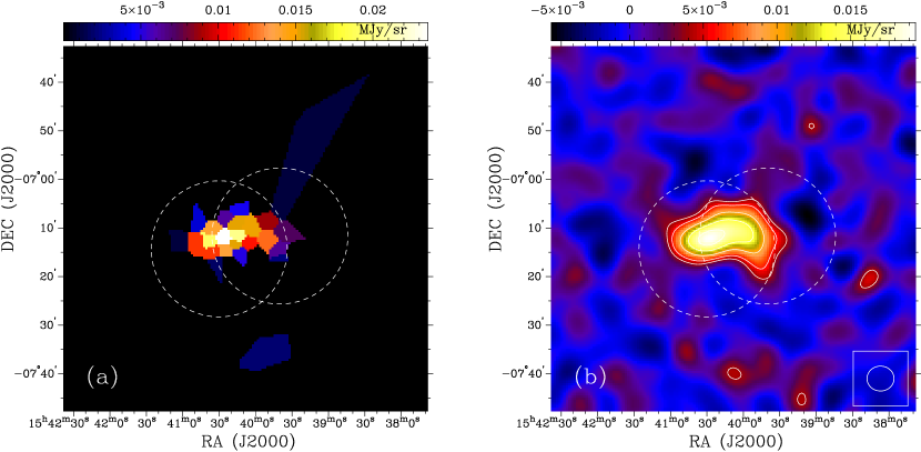
Figure 3: Left: Voronoi model of the visibilities of LDN 1780. This model has 55 polygons. Right: the convolution of the model in the left with the synthetic beam of the data, obtained using natural weights.

2.1 31 GHz Observations

The observations at 31 GHz were carried out with the Cosmic Background Imager (CBI1, Padin et al., 2002), a 13 element interferometer located at an altitude of 5000 m in the Chajnantor plateau in Chile. Each antenna is 0.9 m in diameter and the whole array is mounted on a tracking platform, which rotates in parallactic angle to provide uniform $uv$ coverage. The primary beam has full-width half maximum (FWHM) of 45.2 arcmin at 31 GHz and the angular resolution is $\sim$8 arcmin. The receivers operate in ten frequency channels from 26 to 36 GHz. Each receiver measures either left (L) or right (R) circular polarisation. The interferometer was upgraded during 2006-2007 with 1.4 m dishes (CBI2) to increase temperature sensitivity (Taylor et al. in prep.). The primary beam is 28.2 arcmin FWHM at 31 GHz and the angular resolution was increased to $\sim$4 arcmin.

Table 1 summarises the observations. Both clouds were observed in total intensity mode (all receivers measuring L only). $\zeta$ Oph was observed using CBI1 in a single position while LDN 1780 was observed in two different pointings: L1780E and L1780W by CBI2. The configurations of the CBI1 and CBI2 interferometers result in the ($u,v$) coverage shown in Fig. 1.

We reduced the data using the same routines as those used for CMB data analysis (Pearson et al., 2003; Readhead et al., 2004a, b). Integrations of 8-min on source were accompanied by a trail field, with an offset of 8 arcmin in RA, observed at the same hour angle for the subtraction of local correlated emission (e.g. ground spillover). Flux calibration is tied to Jupiter (with a brightness temperature of $146.6\pm 0.75$ K, Hill et al., 2009).

Table 1: Summary of observations. The coordinates are J2000 and the time quoted is the observation time on-source.

Source	Date	R.A.	decl.	Time
${}^{1}\zeta$ Oph	8/7/04	$16^{\textup{h}}37^{\textup{m}}9^{\textup{s}}.5$	$-10^{\circ}34^{\prime}01^{\prime\prime}$	8000 s
2L1780E	13, 28/4/07	$15^{\textup{h}}40^{\textup{m}}30^{\textup{s}}$	$-07^{\circ}14^{\prime}18^{\prime\prime}$	12000 s
2L1780W	17, 18/4/07	$15^{\textup{h}}39^{\textup{m}}40^{\textup{s}}$	$-07^{\circ}11^{\prime}40^{\prime\prime}$	8000 s

¹: observed with CBI1

²: observed with CBI2

Table 2: Auxiliary data used.

Survey/Telescope	$\lambda$/$\nu$	$\theta^{1}$	Reference
SHASSA	656.3 nm	0.8 arcmin	Gaustad et al. (2001)
Spitzer2	8 $\mu$m	2′′	Fazio et al. (2004)
IRAS/IRIS	12, 25, 60 & 100 $\mu$m	3.8 - 4.3 arcmin	Miville-Deschênes & Lagache (2005)
ISO	100 & 200 $\mu$m	$\sim 1$ arcmin	Kessler et al. (1996)
COBE/DIRBE	100, 140 & 240 $\mu$m	$\sim 0.7^{\circ}$	Hauser et al. (1998)
WMAP	23, 33, 41, 61, & 94 GHz	53 - 13 arcmin	Hinshaw et al. (2009)
PMN	4.85 GHz	$\sim 5$ arcmin	Griffith & Wright (1993)
Stockert	2.72 GHz	$\sim 20$ arcmin	Reif et al. (1984)
HartRAO	2.326 GHz	$\sim 20$ arcmin	Jonas et al. (1998)
Stockert	1.4 GHz	$\sim 35$ arcmin	Reich & Reich (1986)
Parkes	0.408 GHz	51 arcmin	Haslam et al. (1981)

¹: $\theta$ is the angular resolution FWHM

²: Spitzer program 40154

2.1.1 Image reconstruction

The reduced and calibrated visibilities were imaged with the CLEAN algorithm (Högbom, 1974) using the DIFMAP package (Shepherd, 1997). We chose natural weights in order to obtain a deeper restored image. The theoretical noise level (using natural weights, as expected from the visibility weights evaluated from the scatter of individual frames) is 4.9 mJy beam^-1 for $\zeta$ Oph. Fig. 2 shows the CLEAN image of $\zeta$ Oph. This image was then corrected by the primary beam response of CBI1 at 31 GHz (45.2 arcmin). For LDN 1780, we obtained CLEAN images of the two fields. The estimated noise level is 4.3 mJy beam^-1 for L1780E and 3.0 mJy beam^-1 for L1780W. In LDN 1780W a point source, NVSS 153909-065843 (Condon et al., 1998), lies close to the NNW sector of the half-maximum contour of the CBI2 primary beam in Fig. 2. This source allowed us to fix the astrometry of the data which corresponded to an offset of 30^′′ and 56^′′ in R.A. and Dec. These shifts are consistent with the root mean square (rms) pointing accuracy of $\sim$ 0.5 arcmin. The restored CBI2 fields of LDN 1780 were then combined into the weighted mosaic shown on Fig. 2, according to the following formula: $I_{M}(\mathbf{x})={\sum_{p}(w_{p}(\mathbf{x})I_{p}(\mathbf{x})/A_{p}(\mathbf{x}))}/{\sum_{p}w_{p}(\mathbf{x})},$ where $w_{p}(\mathbf{x})=A_{p}^{2}/\sigma_{p}^{2}$, with $p$ the label for the $p$th pointing and $A_{p}(\mathbf{x})$ is the primary beam response.

We also used an alternative method to restore the visibilities in order to check the CLEAN reconstruction. We applied the Voronoi image reconstruction (VIR) from Cabrera et al. (2008), that is well suited to noisy data sets. This novel technique uses a Voronoi tessellation instead of the usual grid, and has the advantage that it is possible to use a smaller number of free parameters during the reconstruction. Moreover, this technique provides the optimal image in a Bayesian sense, so the final image is unique.

Fig. 3 shows the VIR image for LDN 1780. The point source was subtracted from the visibilities before the reconstruction. The result is visibly better because the image negatives are less pronounced than CLEAN (Fig. 2). The largest negative intensity with CLEAN is $-0.007$ MJy/sr whereas with VIR is $-0.005$ MJy/sr. The dynamic range is larger with the VIR reconstruction: 14.8 versus 11.5 from CLEAN. The disadvantage of the VIR reconstruction is the large amount of CPU time required.

Although the VIR reconstruction is better, both techniques gives very similar results. Because of this, we trust the CLEAN reconstruction and used those images for the rest of the investigation.

2.2 Auxiliary data

Table 2 lists the auxiliary data used here. We used images form the Southern H Alpha Sky Survey Atlas (SHASSA), the Spitzer, IRAS, ISO, COBE and WMAP satellites, and low frequency data from the Parkes-MIT-NRAO (PMN) survey, the Rhodes/HartRAO survey, the Stockert radio-telescope, and the Haslam 408 MHz survey. Figures 4 and 5 show large fields of 3^∘ around the two clouds from some of the aforementioned data.

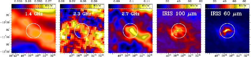
Figure 4: Maps from the auxiliary data around the extraction aperture for $\zeta$ Oph, 3^∘ per side, in J2000 equatorial coordinates. The 1^∘ extraction aperture is shown.

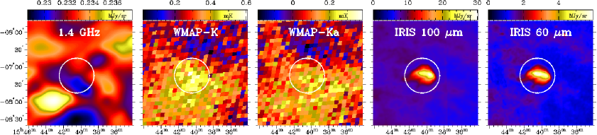
Figure 5: Maps from the auxiliary data around the extraction aperture for LDN 1780, 3^∘ per side, in J2000 equatorial coordinates. The 1^∘ extraction aperture is shown.

Table 3: Flux densities extracted within a 1^∘ circular aperture for $\zeta$ Oph and LDN 1780.

Freq.	Telescope /	$\theta^{1}$	Flux Density	Flux Density
(GHz)	Survey	( arcmin)	$\zeta$ Oph (Jy)	LDN 1780 (Jy)
0.408	Parkes	51	55.4 $\pm$ 5.5	39.6 $\pm$ 4.0
1.4	Stockert	40	66.9 $\pm$ 6.7	56.9 $\pm$ 5.7
2.3	HartRAO	20	19.2 $\pm$ 1.9	9.5 $\pm$ 1.0
2.7	Stockert	20.4	23.7 $\pm$ 2.4	14.9 $\pm$ 1.4
23	WMAP	52.8	7.6 $\pm$ 0.1	1.5 $\pm$ 0.1
33	WMAP	36.6	7.0 $\pm$ 0.2	0.9 $\pm$ 0.2
41	WMAP	30.6	7.0 $\pm$ 0.2	0.6 $\pm$ 0.2
61	WMAP	21	6.2 $\pm$ 0.4	$<$ 1.0 (3$\sigma$)
94	WMAP	13.2	7.2 $\pm$ 0.6	$<$ 2.1 (3$\sigma$)
1249	DIRBE	42	4940 $\pm$ 580	1600 $\pm$ 90
2141	DIRBE	42	7570 $\pm$ 300	4150 $\pm$ 320
2997	DIRBE	42	5600 $\pm$ 200	2900 $\pm$ 160

¹: $\theta$ is the angular resolution FWHM

3 Analysis

3.1 Expected radio emission from H${\alpha}$ emission.

The radio free-free emission must be accurately known in order to quantify the contribution of any dust-related excess emission at GHz-frequencies. One way to estimate its contribution is with the H$\alpha$ emission intensity, provided that this line is the result of in-situ recombination and not scattering by dust.

We used the continuum-corrected H$\alpha$ image from the SHASSA survey (Gaustad et al., 2001). On the region of $\zeta$ Oph, the image was saturated in the position of the star $\zeta$ Oph so re-processing was necessary to get a smooth image. We masked the saturated pixels and interpolated their values using the adjacent pixels. Then, a median filter was applied to remove the field stars. The processed image was corrected for dust absorption using the $E(B-V)$ template from Schlegel et al. (1998) and the extinction curve given by Cardelli et al. (1989). The extinction at H${\alpha}$ is $A$(H${\alpha}$) = 0.82 $A$(V) and using $R_{V}=A(V)/E(B-V)=3.1$ we have that $A$(H${\alpha}$) = 2.54 $E(B-V)$. Finally, we generated a free-free brightness temperature map at 31 GHz using the relationship between H${\alpha}$ intensity and free-free brightness temperature presented in Dickinson et al. (2003) assuming a typical electron temperature $T_{e}=7000$ K, appropriate for the solar neighbourhood.

3.2 Spectral Energy Distribution fit

In this analysis we did not use the CBI data because of the large flux loss on angular scales larger than a few times the synthesised beam. We performed simulations to estimate the flux loss after the reconstruction and we could only recover $\sim$20% of the flux. This would imply that most of the emission from these two clouds is diffuse with respect to the CBI and CBI2 beam.

The images were smoothed to a common resolution of 53 arcmin, the lowest resolution of the data used (WMAP K). We integrated the auxiliary data in a circular aperture 1^∘ in diameter around the central coordinates of the 31 GHz data. Background emission was subtracted integrating in an adjacent region close to the aperture. This is necessary in the case of the low frequency radio data because these surveys have large baseline uncertainties (see for example Reich & Reich, 2009, or the discussion in Davies et al., 1996) In Table 3 we present flux densities for $\zeta$ Oph and LDN 1780 in this aperture.

3.2.1 $\zeta$ Oph

Fig. 6 shows the $\zeta$ Oph SED within a 1^∘ aperture, as tabulated in Table 3. The model is the sum of synchrotron, free-free, thermal dust and spinning dust emissions. We used a synchrotron spectral-index ($T_{b}\propto\nu^{\beta_{S}}$) with $\beta_{S}=-2.7$ (Davies et al., 1996). The free-free power-law is fixed to the predicted brightness temperature at 31 GHz obtained from the H$\alpha$ image. The spectral index used is $\beta_{ff}=-0.12$ (Dickinson et al., 2003). The dominant source of error in the determination of the free-free emission through the H$\alpha$ line is the correction for dust absorption. In Fig. 6, the dotted lines denote limits for the free-free law: the lower is the emission expected from the H$\alpha$ image without dust absorption correction and the upper dotted line is the emission expected with the correction (we assume that all the absorption occurs as a foreground to the H$\alpha$ emission). A modified black body with fixed emissivity index $\beta=1.6$ and 24 K fits the DIRBE 240, 140 and 100 $\mu$m data points. The spinning dust component was fitted using the Ali-Haïmoud et al. (2009) models. The main parameters used in the spinning dust model were $n(H)=100$ cm^-3 and a temperature of 30 K. The emissivities are given in terms of the H column density and we used $N_{H}=1.4\times 10^{21}$cm^-2 (Morton, 1975). The parameters of the dust properties are reasonable for these environments, and were taken from Weingartner & Draine (2001).

On 1^∘ spatial scales, the free-free emission from the Hii region dominates the spectrum in the cm range. The angular resolution of the auxiliary radio data is lower than that of the CBI, so we cannot make a flux comparison on the CBI angular scales.

3.2.2 Surface brightness spectral comparison

The PMN image (Fig. 7) has an angular resolution similar to that of the CBI. However this survey has been high-pass filtered; extended emission on scales larger than $\sim 20$ arcmin is removed (Griffith & Wright, 1993). To make a comparison on CBI angular scales, we simulated visibilities of the PMN image using the same $(u,v)$ coverage of our CBI data. Since large scale modes have been removed from the PMN data, we exclude visibilities at $(u,v)$ radii $<137$ wavelengths (corresponding to angular scales $\lesssim 25$ arcmin). Ideally we should consider only visibilities that correspond to angular scales $\lesssim 15$ arcmin to make a conservative analysis, but doing this excludes most of the visibilities resulting in no signal. Table 4 lists the surface brightness values at the peak of the 31 GHz image. The 4.85/31 GHz spectral index is $\alpha_{4.85}^{31}=0.43\pm 0.20$. We see that $\alpha_{4.85}^{31}$ is significantly different (at the $2.75\sigma$ level) from $-0.12$, the spectral index if the emission at 31 GHz were produced by optically thin free-free emission with $T_{e}\sim 7000$ K. This corresponds to a difference between the 31 GHz intensity and the value expected from a free-free power-law fixed to the PMN point, the non free-free specific intensity, of $I^{\mathrm{nff}}_{31}=I_{31}-I_{4.85}(4.85/31)^{-0.12}=(12\pm 5)$ mJy beam^-1. The significance of the excess is not very high, but we note that this is a comparison at the peak of the 31 GHz map, which is coincident with the bulk of the free-free emission.

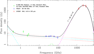
Figure 6: SED of $\zeta$ Oph on 1^∘. The dotted red line shows the maximum and minimum free-free contribution expected given the H$\alpha$ emission. In green is the spinning dust emission from a model of Ali-Haïmoud et al. (2009).

Table 4: Surface brightness values in the peak of the 31 GHz image.

Frequency	Telescope	Surface brightness	Beam size
(GHz)		mJy/beam	(arcmin)
4.85	Parkes 64m	11 $\pm$ 4	5.1
31	CBI	25 $\pm$ 4	7.7

3.2.3 LDN 1780

At the location of LDN 1780, the H$\alpha$ emission present in the SHASSA image is probably scattered light from the Galactic plane (Mattila et al., 2007). Recently, Witt et al. (2010) confirm this result and show that the cloud is embedded in a weaker diffuse H$\alpha$ background, of which approximately half is due to scattered light. In contrast, del Burgo & Cambrésy (2006) state that the H$\alpha$ emission is from the cloud itself and suggest a very high rate of cosmic rays to explain the hydrogen ionisation. Whichever is the case, we can set an upper limit to the free-free contribution using the SHASSA image. The 100, 140 and 240 $\mu$m DIRBE and WMAP 94 GHz points were fitted using a modified black body with fixed emissivity index $\beta=2$. The derived temperature is 17 K. For the spinning dust component we used $n(\text{H})=500$ cm^-3 and $T=20$ K. We estimated the H column density using the extinction map from Schlegel et al. (1998). This estimate used the relation from Bohlin et al. (1978) valid for diffuse clouds: $N$(H+H₂)/$E(B-V)$=5.8$\times 10^{21}$cm^-2mag^-1. We found $N_{H}=3.5\times 10^{21}$cm^-2.

Fig. 8 shows the fit. The pair of dotted lines sets limits on the free-free contribution from the H$\alpha$ data. On the figure are also plotted 3 $\sigma$ upper limits to the contribution at 61 and 94 GHz from the WMAP V and W bands. This SED shows an excess over optically thin free-free emission at cm-wavelengths. The spinning dust model is consistent with the SED in a 1^∘ aperture.

Figure 7: Simulated 4.85 GHz image of $\zeta$ Oph from PMN survey. Contours as in Fig. 2

3.3 Morphological analysis

If dust is responsible for the 31 GHz emission in these clouds, we expect a morphological correspondence with IR emission. A discussion of the infrared emission from dust can be found in Draine & Li (2007) and references therein. The 100 $\mu$m emission is due to grains bigger than 0.01 $\mu$m that are in equilibrium with the interstellar radiation field at a temperature $\sim$10-20 K. On the other hand, the mid-IR emission traces VSGs at $\sim$100 K. They are too hot to be in equilibrium with the environment so these grains are heated stochastically by starlight photons and, given the very small heat capacity of a VSG, a single UV photon increases the particle temperature enough to emit at $\lambda<60~{}\mu$m.

In the SED of $\zeta$ Oph the dominant contribution at 31 GHz is free-free emission. However, inspection of the sky-plane images in Fig. 9 suggests that there is no correspondence between the free-free templates (Fig. 9 a,b) and the 31 GHz contours. The CBI data seem to match better with a combination of free-free and IR emission. We note, however, that the south-eastern arm of the $\zeta$ Oph cloud is slightly offset by $\sim$ 3 arcmin from its IR counterpart. This offset is larger than the rms pointing accuracy of CBI, of order 0.5 arcmin.

In LDN 1780 there are clear differences among the IR images (Fig. 10). By quantifying these differences we can investigate which kind of dust grains (if big grains or VSGs) are responsible for the 31 GHz emission in this cloud.

3.3.1 LDN 1780

3.3.2 Sky plane correlations

Here we investigate sky-plane cross-correlations. For this we used MockCBI, a program which calculates the visibilities $V(u,v)$ of an input image $I_{\nu}(x,y)$ given a reference $(u,v)$ dataset. We computed the visibilities for the IRIS and free-free templates as if they were observed by the CBI with the $(u,v)$ sampling of our data. We reconstructed these visibilities in the same way that we did with the CBI data. Finally, we computed the correlation between the CBI, the IRIS and free-free templates within a square box, 30 arcmin per side, centred at the phase-centre of the 31 GHz data.

Table 5: Sky correlation parameters for $\zeta$ Oph. r is the linear correlation coefficient and a is the proportionality factor between the 31 GHz image and various templates in units of $\mu$K (MJy/sr)^-1. The errors are given by dispersion in the Monte Carlo simulations.

	ff	12 $\mu$m	25 $\mu$m	60 $\mu$m	100 $\mu$m
r	0.7$\pm$0.1	0.5$\pm$0.1	0.4$\pm$0.1	0.5$\pm$0.1	0.4$\pm$0.1
a	460$\pm$100	2.4$\pm$0.5	2.7$\pm$0.1	0.2$\pm$0.1	0.4$\pm$0.1

To estimate the error bars in the correlations, we performed a statistical analysis. We added Gaussian noise to the observed visibilities and reconstructed them 1000 times. Then, we correlated the comparison templates with the noisy mock dataset.

The histogram in Fig. 11a shows the distribution of the Pearson correlation coefficient of the simulated data. The width of the distribution gives us an estimate of the uncertainty in the correlation coefficients and also in the slope of the linear relation between the IR and 31 GHz data. Fig. 11b shows the distribution of the proportionality factor between the emission at 31 GHz and the emission at 100 $\mu$m. Table 5 lists the derived parameters. The errors are from the rms dispersion of the Monte Carlo simulations; they are conservative because of the injection of noise to the data.

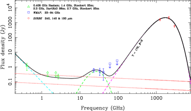
Figure 8: SED of LDN 1780. As in Fig. 6, the red dotted lines show upper and lower limits for the free-free contribution. The symbols with arrows are upper limits (3 $\sigma$). In green is a spinning dust model from a model of Ali-Haïmoud et al. (2009).

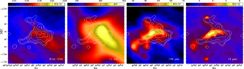
Figure 9: Comparison of different templates of $\zeta$ Oph on the sky plane. From the left to right we show the free-free template obtained from the H$\alpha$ image, the Stockert 2.7 GHz continuum map, the IRAS 100 $\mu$m map (which traces large dust grains), and the IRAS 12 $\mu$m map (which traces very small grains). The contours show the CLEANED image of $\zeta$ Oph. Contours are as in Fig. 2. The south-eastern “arm” of the 31 GHz contours has no counterpart in the free-free template; however it resembles the dust emission.

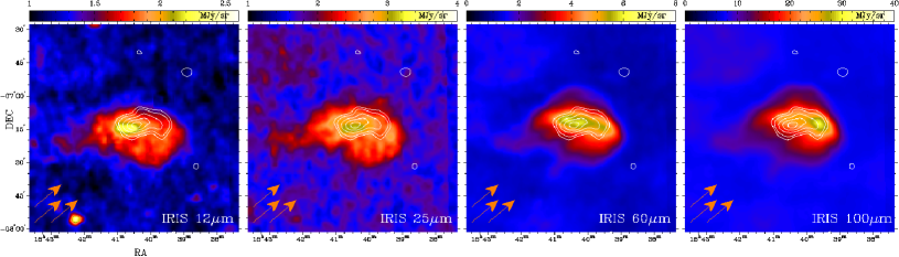
Figure 10: Comparison of the restored CBI2 image of LDN 1780 with IRAS templates. The radio point source NVSS 153909-065843 has been subtracted from the CBI2 data. Contours are as in Fig. 2. Note the morphological differences between the IRAS bands. The arrows in the corner are perpendicular to the Galactic plane and point towards the north Galactic pole.

In the case of $\zeta$ Oph, there are no significant differences between the different IR data and the best correlation is with the free-free template. As we could see in the SED of this cloud (Fig. 6), most of the radio emission is free-free, so it is not a surprise that the best correlation is with the free-free template.

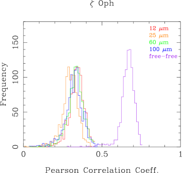
Figure 11: Histograms form the Monte Carlo simulations. Left: histogram of the distribution of the correlation coefficient $r$ for the different templates on $\zeta$ Oph. The correlation with the free-free template is significantly better than the correlation with any dust template. Right: histogram of the distribution of a, the proportionality factor between the 31 GHz and the 100 $\mu$m images. The rms dispersion of these simulations are used as error bars for our results.

In LDN 1780, the correlations between 31 GHz and the IR data show more interesting results. Here, all the IR templates correlate better with the CBI data than in $\zeta$ Oph. The best match is with IRAS 60 $\mu$m, as can be inferred qualitatively from Fig. 10; the Monte Carlo simulations confirm this result (Fig. 12a). The emission at 60 $\mu$m in the diffuse ISM is mainly from VSGs and a 30-40 % contribution from big grains (Desert et al., 1990) so our results favour the idea of a VSGs origin for the cm-wave radiation. Table 6 lists the results.

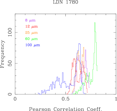
Figure 12: Histograms form the Monte Carlo simulations for LDN 1780. Left: distribution of the correlation coefficient $r$ for the different IR templates. Right: histogram of the distribution of a, the proportionality factor between the 31 GHz and the 100 $\mu$m images.

PAHs emission at 8 & 12 $\mu$m have similar correlation coefficients to that of the 100 $\mu$m emission. However, the emission of VSGs depend on the strength of the IRF. The differences in morphology that appear in this cloud depend both on the distribution of grains within the cloud and in the manner that the cloud is illuminated by the IRF. In the next section we investigate how the IRF illuminates this cloud.

Figure 13: Pixel-by-pixel correlation of CBI data with IRAS 60 $\mu$m and the corrected IRAS 25 $\mu$m templates on LDN 1780. IRAS 60 $\mu$m correlates better in the more diffuse regions while IRAC 25 $\mu$m does better in the peak of the CBI image.

Table 6: Correlation parameters for LDN 1780. r is the linear correlation coefficient and a is the proportionality factor between the 31 GHz image and various templates in units of $\mu$K (MJy/sr)^-1. The errors are given by the dispersion in the Monte Carlo simulations.

	8 $\mu$m	12 $\mu$m	25 $\mu$m	60 $\mu$m	100 $\mu$m
r	0.6$\pm$0.1	0.5$\pm$0.1	0.7$\pm$0.05	0.8$\pm$0.1	0.6$\pm$0.1
a	5.3$\pm$1.0	5.2$\pm$1.4	3.7$\pm$0.9	0.9$\pm$0.2	0.2$\pm$0.1

3.3.3 IRF on LDN 1780

The radio emission from spinning VSGs is fairly independent of the IRF (Draine & Lazarian, 1998b; Ali-Haïmoud et al., 2009; Ysard & Verstraete, 2010). On the other hand, their near-IR (NIR) emission is due to stochastic heating by interstellar photons so it is proportional to the intensity of the radiation field and to the amount of VSGs. Therefore, NIR templates corrected for the IRF would trace better the distribution of VSGs.

The intensity of the radiation field G₀ can be estimated (as in Ysard et al., 2010) from the temperature of the big grains $T_{BG}$ in the cloud. We constructed a temperature map of those grains fitting a modified black body to the ISO 100 & 200 $\mu$m images pixel-by-pixel (at the same resolution). With this temperature map, we calculated G₀ given that:

$$\text{G}_{0}=\left(\frac{T_{BG}}{17.5~{}{\text{K}}}\right)^{\beta+4},$$ (1)

with $\beta=2$. We divided the NIR templates (8 & 12 $\mu$m) by our G₀ map and then repeated the correlations with the 31 GHz data. Again, to estimate error bars, we used the Monte Carlo simulations. The correlations in this case are tighter than with the uncorrected templates; here $r=0.69\pm 0.04$, a 2 $\sigma$ improvement.

4 Comparison of 31 GHz emissivities

One motivation for this work is that the physical conditions in translucent clouds approach that of the cirrus clouds. Here, we compare the radio emission of different clouds in terms of their $N(H)$. To avoid differences in beam sizes and frequencies observed, we choose to compare only sources observed by the CBI, at 31 GHz and scales of 4-8 arcmin. We also calculate an averaged column density for the cirrus clouds using the extinction map from Schlegel et al. (1998) in the positions observed by Leitch et al. (1997) at frequency of 32 GHz and a beam size $\sim$7 arcmin. This beam and frequency are similar to those of the CBI.

In Table 7, we list the radio intensity at the peak of the CBI images, alongside a value for the column density at the same position and the ratio between these two quantities. In Fig. 14 we plot these quantities. The linear fit shown has a slope of $0.54\pm 0.10$ MJy sr^-1 cm^-4 and the correlation coefficient is $r=-0.87$. There seems to be a trend in the direction of diminishing emissivity with increasing column density. Despite the large variations in column density ($\sim$2-3 orders of magnitude), it is interesting that the emissivities of the clouds lie in a small range of $\sim$1 order of magnitude. However, it is worth noting that if the inverse relation we see is real, it will indicate that the anomalous emission is not associated with large dust grains, since their number increases with density, because of dust growth. A similar result was obtained by Lagache (2003), who used WMAP data combined with IR templates and gas tracers in the whole sky on angular scales of 7 deg.

Table 7: Emission parameters for different clouds, all of them but the cirrus were observed by the CBI at 31 GHz. The second column is the column density, the third is the peak intensity at 31 GHz and the fourth is the emissivity at 31 GHz. References are the following: (1) Leitch et al. (1997), (2) Casassus et al. (2006), (3) Casassus et al. (2008), (4) Castellanos et al. (2010)

	$N(H)$ a	$I_{31}$ b	$\epsilon_{31}$ c
Cirrus1	$0.15\pm 0.07$	$6.9\pm 1$	$4.6\pm 2.0$
$\zeta$ Oph	$0.22\pm 0.02$	$9\pm 1$	$4.1\pm 0.6$
LDN 1780	$0.45\pm 0.04$	$16\pm 1$	$3.5\pm 0.4$
LDN 16222	$1.5\pm 0.15$	$30\pm 2$	$2.0\pm 0.2$
$\rho$ Oph3	$5.0\pm 0.50$	$180\pm 20$	$3.2\pm 0.5$
M784	$22.8\pm 0.23$	$210\pm 30$	$0.9\pm 0.1$

^a: $\times 10^{22}$ cm^-2

^b: $\times 10^{-3}$ MJy sr^-1

^c: $\times 10^{-24}$ MJy sr^-1 cm²

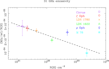
Figure 14: Emissivity at 31 GHz versus column density for different clouds observed with the CBI. The point corresponding to cirrus clouds was obtained as an average from the results of Leitch et al. (1997). The dashed line is the best linear fit to the data.

5 Conclusions

We have presented 31 GHz data of two translucent clouds, $\zeta$ Oph and LDN 1780 with the aim of characterising their radio emissivities. We found an anomalous emission excess in both clouds at 31 GHz on angular scales of $\sim$7 arcmin in $\zeta$ Oph and $\sim$5 arcmin in LDN 1780.

The SED of $\zeta$ Oph on large (1^∘) angular scales is dominated by free-free emission from the associated Hii. Because of this, it is difficult to quantify the contribution from dust to the 31 GHz data. However, when comparing with the optically thin free-free extrapolated from the 5 GHz PMN image, we find a 2.4 $\sigma$ excess at 31 GHz on spatial scales of 7 arcmin in surface brightness.

In the SED of LDN 1780 we see an excess on 1^∘ angular scales. The free-free contribution in this cloud is expected to be very low; the H$\alpha$ emission may be scattered light from the IRF, so it would not have a radio counterpart. A spinning dust component can explain the anomalous emission excess in the SED. Correlations between the cm-wave data and IR-templates shows a trend favouring IRAS 25 & 60 $\mu$m. The best match in this case is with IRAS 60 $\mu$m although the peak of the CBI image is best matched by IRAC 8 $\mu$m. We corrected the IRAC 8 $\mu$m and IRAS 12 $\mu$m by the IRF and found a tighter correlation with these corrected templates. In the spinning dust models, the VSGs dominate the radio emission. Our results support this mechanism as the origin for the anomalous emission in this cloud.

The 31 GHz emissivities found in both clouds are similar and have intermediate values between the cirrus clouds and the dark clouds. The emissivity variations with column density are small, although we find an indication of an inverse relationship, which would further support a VSGs origin for the cm-emission. The anomalous foreground which contaminates CMB data comes from cirrus clouds at typically high Galactic latitudes. Here, we see that there is not a large difference between the radio emissivity of cirrus and translucent clouds on 7 arcmin angular scales. Because of this similarity, translucent clouds are good places to investigate the anomalous CMB foreground.

References

- Ali-Haïmoud et al. (2009) Ali-Haïmoud, Y., Hirata, C. M., & Dickinson, C. 2009, MNRAS, 395, 1055
- Ami Consortium et al. (2009) Ami Consortium, et al. 2009, MNRAS, 394, L46
- Banday et al. (2003) Banday, A. J., Dickinson, C., Davies, R. D., Davis, R. J., & Górski, K. M. 2003, MNRAS, 345, 897
- Bennett et al. (1992) Bennett, C. L., et al. 1992, ApJ, 396, L7
- Bennett et al. (2003) Bennett, C. L., et al. 2003, ApJS, 148, 97
- Bevington & Robinson (2003) Bevington, P. R., & Robinson, D. K. 2003, Data reduction and error analysis for the physical sciences, 3rd ed., by Philip R. Bevington, and Keith D. Robinson. Boston, MA: McGraw-Hill, ISBN 0-07-247227-8, 2003.,
- Black & Dalgarno (1977) Black, J. H., & Dalgarno, A. 1977, ApJS, 34, 405
- Bohlin et al. (1978) Bohlin, R. C., Savage, B. D., & Drake, J. F. 1978, ApJ, 224, 132
- Boulanger & Perault (1988) Boulanger, F., & Perault, M. 1988, ApJ, 330, 964
- Cabrera et al. (2008) Cabrera, G. F., Casassus, S., & Hitschfeld, N. 2008, ApJ, 672, 1272
- Cardelli et al. (1989) Cardelli, J. A., Clayton, G. C., & Mathis, J. S. 1989, ApJ, 345, 245
- Casassus et al. (2004) Casassus, S., Readhead, A. C. S., Pearson, T. J., Nyman, L.-Å., Shepherd, M. C., & Bronfman, L. 2004, ApJ, 603, 599
- Casassus et al. (2006) Casassus, S., Cabrera, G. F., Förster, F., Pearson, T. J., Readhead, A. C. S., & Dickinson, C. 2006, ApJ, 639, 951
- Casassus et al. (2007) Casassus, S., Nyman, L.-Å., Dickinson, C., & Pearson, T. J. 2007, MNRAS, 382, 1607
- Casassus et al. (2008) Casassus, S., et al. 2008, MNRAS, 391, 1075
- Castellanos et al. (2010) Castellanos, P., et al. 2010, arXiv:1010.2581
- Condon et al. (1998) Condon, J. J., Cotton, W. D., Greisen, E. W., Yin, Q. F., Perley, R. A., Taylor, G. B., & Broderick, J. J. 1998, AJ, 115, 1693
- Davies et al. (2006) Davies, R. D., Dickinson, C., Banday, A. J., Jaffe, T. R., Górski, K. M., & Davis, R. J. 2006, MNRAS, 370, 1125
- Davies et al. (1996) Davies, R. D., Watson, R. A., & Gutierrez, C. M. 1996, MNRAS, 278, 925
- de Oliveira-Costa et al. (1997) de Oliveira-Costa, A., Kogut, A., Devlin, M. J., Netterfield, C. B., Page, L. A., & Wollack, E. J. 1997, ApJ, 482, L17
- de Oliveira-Costa et al. (1999) de Oliveira-Costa, A., Tegmark, M., Gutierrez, C. M., Jones, A. W., Davies, R. D., Lasenby, A. N., Rebolo, R., & Watson, R. A. 1999, ApJ, 527, L9
- de Oliveira-Costa et al. (2002) de Oliveira-Costa, A., et al. 2002, ApJ, 567, 363
- de Oliveira-Costa et al. (2004) de Oliveira-Costa, A., Tegmark, M., Davies, R. D., Gutiérrez, C. M., Lasenby, A. N., Rebolo, R., & Watson, R. A. 2004, ApJ, 606, L89
- del Burgo & Cambrésy (2006) del Burgo, C., & Cambrésy, L. 2006, MNRAS, 368, 1463
- Desert et al. (1990) Desert, F.-X., Boulanger, F., & Puget, J. L. 1990, A&A, 237, 215
- Dickinson et al. (2003) Dickinson, C., Davies, R. D., & Davis, R. J. 2003, MNRAS, 341, 369
- Dickinson et al. (2007) Dickinson, C., Davies, R. D., Bronfman, L., Casassus, S., Davis, R. J., Pearson, T. J., Readhead, A. C. S., & Wilkinson, P. N. 2007, MNRAS, 379, 297
- Dickinson et al. (2009) Dickinson, C., et al. 2009, ApJ, 690, 1585
- Draine & Lazarian (1998a) Draine, B. T., & Lazarian, A. 1998, ApJ, 494, L19
- Draine & Lazarian (1998b) Draine, B. T., & Lazarian, A. 1998, ApJ, 508, 157
- Draine & Lazarian (1999) Draine, B. T., & Lazarian, A. 1999, ApJ, 512, 740
- Draine & Li (2007) Draine, B. T., & Li, A. 2007, ApJ, 657, 810
- Fazio et al. (2004) Fazio, G. G., et al. 2004, ApJS, 154, 10
- Fernández-Cerezo et al. (2006) Fernández-Cerezo, S., et al. 2006, MNRAS, 370, 15
- Finkbeiner (2004) Finkbeiner, D. P. 2004, ApJ, 614, 186
- Finkbeiner et al. (2004) Finkbeiner, D. P., Langston, G. I., & Minter, A. H. 2004, ApJ, 617, 350
- Franco (1989) Franco, G. A. P. 1989, A&A, 223, 313
- Gaustad et al. (2001) Gaustad, J. E., McCullough, P. R., Rosing, W., & Van Buren, D. 2001, PASP, 113, 1326
- Giardino et al. (2002) Giardino, G., Banday, A. J., Górski, K. M., Bennett, K., Jonas, J. L., & Tauber, J. 2002, A&A, 387, 82
- Griffith & Wright (1993) Griffith, M. R., & Wright, A. E. 1993, AJ, 105, 1666
- Hamaker et al. (1996) Hamaker, J. P., Bregman, J. D., & Sault, R. J. 1996, A&AS, 117, 137
- Haslam et al. (1981) Haslam, C. G. T., Klein, U., Salter, C. J., Stoffel, H., Wilson, W. E., Cleary, M. N., Cooke, D. J., & Thomasson, P. 1981, A&A, 100, 209
- Haslam et al. (1982) Haslam, C. G. T., Salter, C. J., Stoffel, H., & Wilson, W. E. 1982, A&AS, 47, 1
- Hauser et al. (1998) Hauser, M. G., et al. 1998, ApJ, 508, 25
- Hill et al. (2009) Hill, R. S., et al. 2009, ApJS, 180, 246
- Hinshaw et al. (2009) Hinshaw, G., et al. 2009, ApJS, 180, 225
- Högbom (1974) Högbom, J. A. 1974, A&AS, 15, 417
- Jørgensen et al. (2006) Jørgensen, J. K., et al. 2006, ApJ, 645, 1246
- Jonas et al. (1998) Jonas, J. L., Baart, E. E., & Nicolson, G. D. 1998, MNRAS, 297, 977
- Kessler et al. (1996) Kessler, M. F., et al. 1996, A&A, 315, L27
- Kogut et al. (1996a) Kogut, A., Banday, A. J., Bennett, C. L., Gorski, K. M., Hinshaw, G., & Reach, W. T. 1996, ApJ, 460, 1
- Kogut et al. (1996b) Kogut, A., Banday, A. J., Bennett, C. L., Gorski, K. M., Hinshaw, G., Smoot, G. F., & Wright, E. I. 1996, ApJ, 464, L5
- Lagache et al. (1999) Lagache, G., Abergel, A., Boulanger, F., Désert, F. X., & Puget, J.-L. 1999, A&A, 344, 322
- Lagache (2003) Lagache, G. 2003, A&A, 405, 813
- Leitch et al. (1997) Leitch, E. M., Readhead, A. C. S., Pearson, T. J., & Myers, S. T. 1997, ApJ, 486, L23
- Lombardi & Alves (2001) Lombardi, M., & Alves, J. 2001, A&A, 377, 1023
- Low et al. (1984) Low, F. J., et al. 1984, ApJ, 278, L19
- Magnani et al. (1985) Magnani, L., Blitz, L., & Mundy, L. 1985, ApJ, 295, 402
- Mathis et al. (1983) Mathis, J. S., Mezger, P. G., & Panagia, N. 1983, A&A, 128, 212
- Mattila et al. (2007) Mattila, K., Juvela, M., & Lehtinen, K. 2007, ApJ, 654, L131
- Meyer (1969) Meyer, P. 1969, ARA&A, 7, 1
- Miville-Deschênes et al. (2002) Miville-Deschênes, M.-A., Boulanger, F., Joncas, G., & Falgarone, E. 2002, A&A, 381, 209
- Miville-Deschênes et al. (2008) Miville-Deschênes, M.-A., Ysard, N., Lavabre, A., Ponthieu, N., Macías-Pérez, J. F., Aumont, J., & Bernard, J. P. 2008, A&A, 490, 1093
- Miville-Deschênes & Lagache (2005) Miville-Deschênes, M.-A., & Lagache, G. 2005, ApJS, 157, 302
- Morton (1975) Morton, D. C. 1975, ApJ, 197, 85
- Mukherjee et al. (2001) Mukherjee, P., Jones, A. W., Kneissl, R., & Lasenby, A. N. 2001, MNRAS, 320, 224
- Mukherjee et al. (2003) Mukherjee, P., Coble, K., Dragovan, M., Ganga, K., Kovac, J., Ratra, B., & Souradeep, T. 2003, ApJ, 592, 692
- Padin et al. (2002) Padin, S., et al. 2002, PASP, 114, 83
- Parravano et al. (2003) Parravano, A., Hollenbach, D. J., & McKee, C. F. 2003, ApJ, 584, 797
- Pearson et al. (2003) Pearson, T. J., et al. 2003, ApJ, 591, 556
- Peretto & Fuller (2009) Peretto, N., & Fuller, G. A. 2009, A&A, 505, 405
- Perryman et al. (1997) Perryman, M. A. C., et al. 1997, A&A, 323, L49
- Readhead et al. (2004a) Readhead, A. C. S., et al. 2004, ApJ, 609, 498
- Readhead et al. (2004b) Readhead, A. C. S., et al. 2004, Science, 306, 836
- Reich & Reich (2009) Reich, W., & Reich, P. 2009, IAU Symposium, 259, 603
- Reich & Reich (1986) Reich, P., & Reich, W. 1986, A&AS, 63, 205
- Reif et al. (1984) Reif, K., Steffen, P., & Reich, W. 1984, Kleinheubacher Berichte, 27, 295
- Ridderstad et al. (2006) Ridderstad, M., Juvela, M., Lehtinen, K., Lemke, D., & Liljeström, T. 2006, A&A, 451, 961
- Rybicki & Lightman (1986) Rybicki, G. B., & Lightman, A. P. 1986, Radiative Processes in Astrophysics, by George B. Rybicki, Alan P. Lightman, pp. 400. ISBN 0-471-82759-2. Wiley-VCH , June 1986.,
- Schlegel et al. (1998) Schlegel, D. J., Finkbeiner, D. P., & Davis, M. 1998, ApJ, 500, 525
- Sellgren et al. (1985) Sellgren, K., Allamandola, L. J., Bregman, J. D., Werner, M. W., & Wooden, D. H. 1985, ApJ, 299, 416
- Shepherd (1997) Shepherd, M. C. 1997, Astronomical Data Analysis Software and Systems VI, 125, 77
- Simon et al. (2006) Simon, R., Rathborne, J. M., Shah, R. Y., Jackson, J. M., & Chambers, E. T. 2006, ApJ, 653, 1325
- Snow & McCall (2006) Snow, T. P., & McCall, B. J. 2006, ARA&A, 44, 367
- Stark (1990) Stark, R. 1990, A&A, 230, L25
- Stark et al. (1994) Stark, R., Dickey, J. M., Burton, W. B., & Wennmacher, A. 1994, A&A, 281, 199
- Taylor et al. (1999) Taylor, G. B., Carilli, C. L., & Perley, R. A. 1999, Synthesis Imaging in Radio Astronomy II, 180,
- Turner (1994) Turner, B. E. 1994, The First Symposium on the Infrared Cirrus and Diffuse Interstellar Clouds, 58, 307
- van Dishoeck & Black (1986) van Dishoeck, E. F., & Black, J. H. 1986, ApJS, 62, 109
- Viala et al. (1988) Viala, Y. P., Roueff, E., & Abgrall, H. 1988, A&A, 190, 215
- Watson et al. (2005) Watson, R. A., Rebolo, R., Rubiño-Martín, J. A., Hildebrandt, S., Gutiérrez, C. M., Fernández-Cerezo, S., Hoyland, R. J., & Battistelli, E. S. 2005, ApJ, 624, L89
- Weingartner & Draine (2001) Weingartner, J. C., & Draine, B. T. 2001, ApJ, 548, 296
- Wilson et al. (2009) Wilson, T. L., Rohlfs, K., Hüttemeister, S. 2009, Tools of Radio Astronomy, by Thomas L. Wilson; Kristen Rohlfs and Susanne Hüttemeister. ISBN 978-3-540-85121-9. Published by Springer-Verlag, Berlin, Germany, 2009.
- Witt et al. (2010) Witt, A. N., Gold, B., Barnes, F. S., DeRoo, C. T., Vijh, U. P., & Madsen, G. J. 2010, ApJ, 724, 1551
- Ysard & Verstraete (2010) Ysard, N., & Verstraete, L. 2010, A&A, 509, A12
- Ysard et al. (2010) Ysard, N., Miville-Deschênes, M. A., & Verstraete, L. 2010, A&A, 509, L1